EVLA Advanced Topics 3C391

Continuum Observations Data Reduction Tutorial: 3C 391---Advanced Topics

In this document, we discuss various "advanced topics" for further reduction of the 3C 391 continuum data. This tutorial assumes that the reader already has some familiarity with basic continuum data reduction, such as should have been obtained Continuum Data Reduction Tutorial on the first day of the NRAO Synthesis Imaging Workshop data reduction tutorials. If one did not participate in the EVLA Continuum Data Reduction Tutorial, one could use the script extractor to generate a CASA reduction script and process the data to form an initial image. Current experience on a standard desktop computer suggests that such a data set could be processed in 30 min. or less.

Image Analysis and Manipulation

This topic is perhaps not "advanced," but it appears to fit more naturally here. It is assumed that an image 3c391_ctm_spw0_IQUV.image, resulting from the Continuum Data Reduction Tutorial exists.

The three most basic analyses are to determine the peak brightness, the flux density, and the image noise level. These are useful measures of how well one's imaging efforts are in approaching the thermal noise limit or in reproducing what is already known about a source. Additional discussion of image analysis and manipulation, including the combination of multiple images, mathematical operations on images, and much more can be found in Image Analysis in the CASA Reference Book.

The most straightforward statistic is the peak brightness, which is determined by imstat.

imstat(imagename='3c391_ctm_spw0_IQUV.image',stokes='')

• stokes=' ' : This example determines the peak brightness in the entire image, which has all four Stokes planes. If one wanted to determine the peak brightness in just, say, the Stokes V image, one would set stokes='V'.

The other two statistics require slightly more care. The flux density of a source is determined by integrating its brightness or intensity over some solid angle, i.e., [math]\displaystyle{ S = \int d\Omega I }[/math], where [math]\displaystyle{ I }[/math] is the intensity (measured in units of Jy/beam), [math]\displaystyle{ \Omega }[/math] is the solid angle of the source (e.g., number of synthesized beams), and [math]\displaystyle{ S }[/math] is the flux density (measured in units of Jy). In general, if the noise is well-behaved in one's image, when averaged over a reasonable solid angle, the noise contribution should approach 0 Jy. If that is the case, then the flux density of the source is also reported by imstat. However, there are many cases for which a noise contribution of 0 Jy may not be a safe assumption. If one's source is in a complicated region (e.g., a star formation region, the Galactic center, near the edge of a galaxy), a better estimate of the source's flux density will be obtained by limiting carefully the solid angle over which the integration is performed.

polygon region button selection

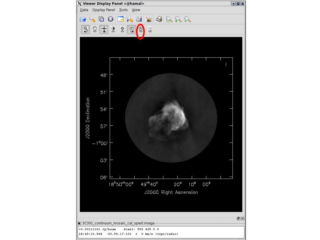
Open viewer and use it to display an image, such as 3c391_ctm_spw0_IQUV.image. One can choose the function assigned to each mouse button; assign 'polygon region' to a desired mouse button (e.g., right button) by selecting the icon shown in the figure to the right with the desired mouse button.

Using the mouse button just assigned to 'polygon region', outline the supernova remnant. Double click inside of that region, and the statistics will be reported. In fact, two sets of statistics will be returned. In the window one is using for casapy itself will be a set of statistics determined over the entire image cube; a new pop-up window will also appear, showing the image statistics for the particular Stokes plane being displayed in the viewer. One of the statistics reported will be the flux density within the region selected. (For the record, one of the authors of this document found a flux density of about 2.4 Jy.)

polygonal region for determining image statistics

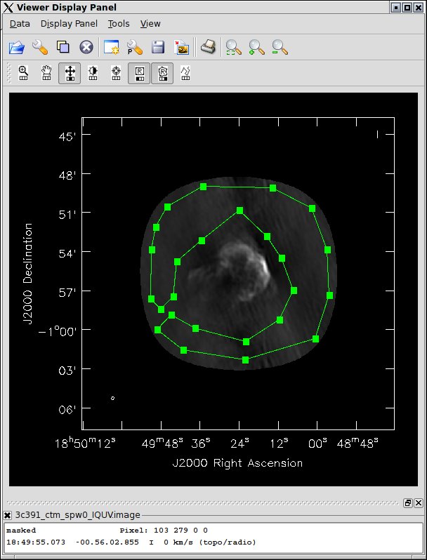
By contrast, for the rms noise level, one wants to exclude the source's emission to the extent possible, as the source's emission will bias the estimated noise level high. One can repeat the procedure above, defining a polygonal region, then double clicking inside it, to determine the statistics. In the region illustrated in the figure to the right, one of the authors of this document found an rms noise level of 1.4 mJy/beam.

Polarization Imaging

data display options for total intensity contours

In the previous data reduction tutorial, a full polarization imaging cube of 3C 391 was constructed. This cube has 3 dimensions, the standard two angular dimensions (right ascension, declination) and a third dimension containing the polarization information. Considering the image cube as a matrix, [math]\displaystyle{ Image[l,m,p] }[/math], the [math]\displaystyle{ l }[/math] and [math]\displaystyle{ m }[/math] axis describe the sky brightness or intensity for the given [math]\displaystyle{ p }[/math] axis. If one opens the viewer and loads the 3C 391 continuum image, the default view contains an "animator" or pane with movie controls. One can step through the polarization axis, displaying the images for the different polarizations.

As constructed, the image contains four polarizations, for the four Stokes parameters, I, Q, U, and V. Recalling the lectures, Q and U describe the linear polarization and V describes the circular polarization. Specifically, Q describes the amount of linear polarization aligned with a given axis, and U describes the amount of linear polarization at a 45 deg angle to that axis. The V parameter describes the amount of circular polarization, with the sign (positive or negative) describing the sense of the circular polarization (right- or left-hand circularly polarized).

In general, few celestial sources are expected to show circular polarization, with the notable exception of masers, while terrestrial and satellite sources are often highly circularly polarized. The V image is therefore often worth forming because any V emission could be indicative of unflagged RFI within the data (or problems with the calibration!).

Because the Q and U images both describe the amount of linear polarization, it is more common to work with a linear polarization intensity image, [math]\displaystyle{ P = \sqrt{Q^2 +U^2} }[/math]. ([math]\displaystyle{ P }[/math] can also be denoted by [math]\displaystyle{ L }[/math].) Also important can be the polarization position angle [math]\displaystyle{ tan 2\chi = U/Q }[/math].

data display options for position angle vectors

The relevant task is immath, with specific examples for processing of polarization images given in Polarization Manipulation. The steps are the following.

1. Extract the I, Q, U, V planes from the full Stokes image cube, forming separate images for each Stokes parameter.

# In CASA
immath(imagename='3c391_ctm_spw0_IQUV.image',outfile='3c391_ctm_spw0.I',expr='IM0',stokes='I')
immath(imagename='3c391_ctm_spw0_IQUV.image',outfile='3c391_ctm_spw0.Q',expr='IM0',stokes='Q')
immath(imagename='3c391_ctm_spw0_IQUV.image',outfile='3c391_ctm_spw0.U',expr='IM0',stokes='U')
immath(imagename='3c391_ctm_spw0_IQUV.image',outfile='3c391_ctm_spw0.V',expr='IM0',stokes='V')

2. Combine the Q and U images using the mode='poli' option of immath to form the linear polarization image.

# In CASA
immath(mode='poli',imagename=['3c391_ctm_spw0.Q','3c391_ctm_spw0.U'],outfile='3c391_ctm_spw0.P',sigma='0.08mJy/beam')

To correct for bias (the P image does not obey Gaussian statistics), we must supply the noise level in the Stokes Q and U images (these should be similar), using the sigma parameter. These noise levels can be estimated as described in the Image Analysis and Manipulation section above.

3. If desired, combine the Q and U images using the mode='pola' option of immath to form the polarization position angle image. Because the polarization position angle is derived from the tangent function, the order in which the Q and U images are specified is important.

# In CASA
immath(mode='pola',imagename=['3c391_ctm_spw0.Q','3c391_ctm_spw0.U'],outfile='3c391_ctm_spw0.X',sigma='0.08mJy/beam',
    polithresh='0.4mJy/beam')

Again, we supply the noise level. To avoid displaying the position angle of noise, we can set a threshold intensity of the linear polarization for above which we wish to calculate the polarization angle, using the polithresh parameter. An appropriate level here might be the [math]\displaystyle{ 5\sigma }[/math] level of 0.4 mJy/beam.

4. If desired, form the fractional linear polarization image, defined as P/I.

# In CASA
immath(outfile='3c391_ctm_spw0.F',imagename=['3c391_ctm_spw0.I','3c391_ctm_spw0.Q','3c391_ctm_spw0.U'],mode='evalexpr',
    expr='sqrt((IM1^2-IM2^2)/IM0[IM0>2.7e-3]^2)')

Since the total intensity image can (and hopefully does) approach zero in regions free of source emission, dividing by the total intensity can produce very high pixel values in these regions. We therefore wish to restrict our fractional polarization image to regions containing real emission, which we do by setting a threshold in the total intensity image, which in this case corresponds to three times the noise level. The computation of the polarized intensity is specified by expr='sqrt((IM1^2-IM2^2)/IM0[IM0>2.7e-3]^2)' , with the expression in square brackets setting the threshold in IM0 (the total intensity image). Note that IM0, IM1 and IM2 correspond to the three files listed in the imagename array, in that order. The order in which the different images are specified is therefore critical once again.

One can then view these various images using viewer. It is instructive to display the I, P and X images (total intensity, total linearly polarized intensity, and polarization position angle) together, to show how the polarized emission relates to the total intensity, and how the magnetic field is structured. We can do this using the viewer.

• Begin by loading the linear polarization image in the viewer:

# In CASA
viewer('3c391_ctm_spw0.P')

• Next, load the total intensity image as a contour image. In the viewer panel, hit the "Open" icon (the leftmost button in the top row of icons in the viewer). This will bring up a 'Load Data' GUI showing all images and MS in the current directory. Select the total intensity image (3c391_ctm_spw0.I) and click the 'Contour Map' button on the right hand side.
• Finally, load the polarization position angle image (3c391_ctm_spw0.X) as a vector map.

While we set the polithresh parameter when we created the position angle (X) image, a digression here is instructive in the use of LEL Expressions. Had we not set this parameter, the position angle would have been derived for all pixels within the full IQUV image cube. There is only polarized emission from a limited subset of pixels within this image. Therefore, to avoid plotting vectors corresponding to the position angle of pure noise, we would now wish to select only the regions where the polarized intensity is brighter than some threshold value. To do this, we would use a LEL (Lattice Expression Language) Expression in the 'Load Data' GUI. For our chosen threshold of 0.4 mJy (the 5 sigma level in the P image), we would paste the expression '3C391_ctm_spw0.X'['3C391_ctm_spw0.P'>0.0004] into the LEL Expression box in the GUI, and click the 'Vector Map' button. This would load the vectors only for regions where [math]\displaystyle{ P\gt 0.4 }[/math] mJy.

final full-polarization image of 3C391

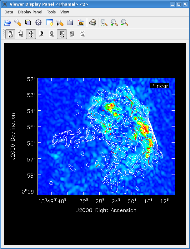
While we now have all three images loaded into the viewer (the polarized intensity (3c391_ctm_spw0.P) in color, the total intensity (3c391_ctm_spw0.I) as a contour map, and the polarization position angle (3c391_ctm_spw0.X) as a vector map), we still wish to optimize the display for ease of interpretation.

• Change the image transfer function. Hold down the middle mouse button and move the mouse until the color scale is optimized for the display of the polarized intensity.
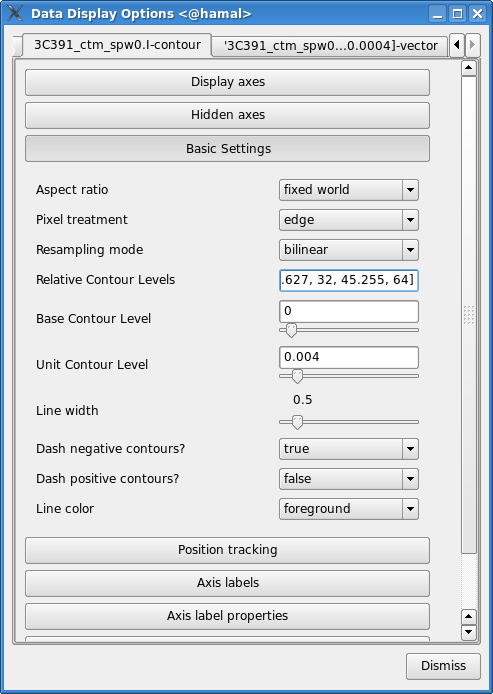
• Change the contour levels. Click the wrench icon to open a 'Data Display Options' GUI. This will have 3 tabs, corresponding to the three images loaded. Select the total intensity tab (3c391_ctm_spw0.I). Change the relative contour levels from the default levels of [0.2,0.4,0.6,0.8,1.0] to powers of [math]\displaystyle{ \sqrt{2} }[/math], including a couple of negative contours at the beginning to demonstrate the image quality. An appropriate set of levels might be [-1.414,-1,1,1.414,2,2.828,4,5.657,8,11.314,16,22.627,32,45.255,64]. These levels will multiply the Unit Contour Level, which we set at some multiple of the rms noise in the total intensity image. An appropriate value might be 0.0024 Jy ([math]\displaystyle{ 3\sigma }[/math]).
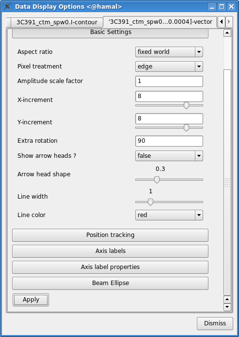
• Change the vector spacing and color, and rotate the vectors. The polarization position angle as calculated is the electric vector position angle (EVPA). If we are interested in the orientation of the magnetic field, then for an optically thin source, the magnetic field orientation is perpendicular to the EVPA, so we must rotate the vectors by [math]\displaystyle{ 90^{\circ} }[/math]. Select the vector image tab in the 'Data Display Options' GUI (labeled as the LEL expression we entered in the Load Data GUI) and enter 90 in the Extra rotation box. If the vectors appear too densely packed on the image, change the spacing of the vectors by setting X-increment and Y-increment to a larger value (8 might be appropriate here). Finally, to be able to distinguish the vectors from the total intensity contours, change the color of the vectors by selecting a different Line color (red might be a good choice).

Now that we have altered the display to our satisfaction, it remains only to zoom in to the region containing the emission. Close the animator tab in the viewer, and then drag out a rectangular region around the supernova remnant with your left mouse button. Double-click to zoom in to that region. This will give you a final image looking something like that shown at right.

Spectral Index Imaging

The spectral index, defined as the slope of the radio spectrum between two different frequencies, [math]\displaystyle{ \log(S_{\nu_1}/S_{\nu_2})/\log(\nu_1/\nu_2) }[/math], is a useful analytical tool which can convey information about the emission mechanism, the optical depth of the source or the underlying energy distribution of synchrotron-radiating electrons.

Having used immath to manipulate the polarization images, the reader should now have some familiarity with performing mathematical operations within CASA. immath also has a special mode for calculating the spectral index, mode='spix' . The two input images at different frequencies should be provided using the parameter (in this case, the Python list) imagename. With this information, it is left as an exercise for the reader to create a spectral index map.

The two input images could be the two different spectral windows from the 3C391 continuum data set. If the higher-frequency spectral window (spw1) has not yet been reduced, then two images made with different channel ranges from the lower spectral window, spw0, should suffice. In this latter case, the extreme upper and lower channels are suggested, to provide a sufficient lever arm in frequency to measure a believable spectral index.

Self-Calibration

Recalling the lectures, even after the initial calibration using the amplitude calibrator and the phase calibrator, there are likely to be residual phase and/or amplitude errors in the data. Self-calibration is the process of using an existing model, often constructed by imaging the data itself. Provided that sufficient visibility data have been obtained, and this is essentially always the case with the EVLA (and often the VLBA, and should be with ALMA), the system of equations is wildly over-constrained for the number of unknowns.

More specifically, the observed visibility data on the [math]\displaystyle{ i }[/math]-[math]\displaystyle{ j }[/math] baseline can be modeled as

[math]\displaystyle{ V'_{ij} = G_i G^*_j V_{ij} }[/math]

where [math]\displaystyle{ G_i }[/math] is the complex gain for the [math]\displaystyle{ i^{\mathrm{th}} }[/math] antenna and [math]\displaystyle{ V_{ij} }[/math] is the "true" visibility. For an array of [math]\displaystyle{ N }[/math] antennas, at any given instant, there are [math]\displaystyle{ N(N-1)/2 }[/math] visibility data, but only [math]\displaystyle{ N }[/math] gain factors. For an array with a reasonable number of antennas, [math]\displaystyle{ N }[/math] >~ 8, solutions to this set of coupled equations converge quickly.

There is a small amount of discussion in the CASA Reference Manual on self calibration. In self-calibrating data, it is useful to keep in mind the structure of a Measurement Set: there are three columns of interest for an MS, the DATA column, the MODEL column, and the CORRECTED_DATA column. In normal usage, as part of the initial split, the CORRECTED_DATA column is set equal to the DATA column. The self-calibration procedure is then

• Produce an image (clean) using the CORRECTED_DATA column.
• Derive a series of gain corrections (gaincal) by comparing the DATA columns and the Fourier transform of the image, which is stored in the MODEL column. These corrections are stored in an external table.
• Apply these corrections (applycal) to the DATA column, to form a new CORRECTED_DATA column, overwriting the previous contents of CORRECTED_DATA.

The following example begins with the standard data set, 3c391_ctm_mosaic_spw0.ms, resulting from the [3C391 Continuum Tutorial]. A model image is generated (3c391_ctm_spw0_IQUV.image), this model is used to generate a series of gain corrections (stored in 3C391_ctm_mosaic_spw0.G2), those gain corrections are applied to the data to form a set of self-calibrated data, and new image is then formed (3c391_ctm_spw0_IQUV_G2.image).

#In CASA
clean(vis='3c391_ctm_mosaic_spw0.ms',imagename='3c391_ctm_spw0_IQUV',
      field='',spw='',
      mode='mfs',
      niter=5000,
      gain=0.1,threshold='0.0mJy',
      psfmode='clarkstokes',
      imagermode='mosaic',ftmachine='mosaic',
      multiscale=[0, 6, 18, 54],smallscalebias=0.9,
      interactive=True,
      imsize=[576,576],cell=['2.5arcsec','2.5arcsec'],
      stokes='IQUV',
      weighting='briggs',robust=0.0,
      calready=True)

gaincal(vis='3c391_ctm_mosaic_spw0.ms',caltable='3C391_ctm_mosaic_spw0.G2',
        field='',spw='',selectdata=False,
        solint='30s',refant='ea21',minblperant=4,minsnr=3,
        solnorm=True,gaintype='G',calmode='p',append=False)

applycal(vis='3c391_ctm_mosaic_spw0.ms',
         field='',spw='',selectdata=False,
         gaintable= ['3c391_ctm_mosaic_spw0.G2'],gainfield=[''],interp=['nearest'])

clean(vis='3c391_ctm_mosaic_spw0.ms',imagename='3c391_ctm_spw0_IQUV_G2',
      field='',spw='',
      mode='mfs',
      niter=5000,
      gain=0.1,threshold='0.0mJy',
      psfmode='clarkstokes',
      imagermode='mosaic',ftmachine='mosaic',
      multiscale=[0, 6, 18, 54],smallscalebias=0.9,
      interactive=True,
      imsize=[576,576],cell=['2.5arcsec','2.5arcsec'],
      stokes='IQUV',
      weighting='briggs',robust=0.0,
      calready=True)

Commonly, this procedure is applied multiple times. The number of iterations is determined by a combination of the data quality and number of antennas in the array, the structure of the source, the extent to which the original self-calibration assumptions are valid, and the user's patience. With reference to the original self-calibration equation above, if the observed visibility data cannot be modeled well by this equation, no amount of self-calibration will help. A not-uncommon limitation for moderately high dynamic range imaging is that there may be baseline-based factors that modify the "true" visibility. If the corruptions to the "true" visibility cannot be modeled as antenna-based, as they are above, self-calibration won't help.

Self-calibration requires experimentation. Do not be afraid to dump an image, or even a set of gain corrections, change something and try again. Having said that, here are several general comments or guidelines:

• Bookkeeping is important! Suppose one conducts 9 iterations of self-calibration. Will it be possible to remember one month later (or maybe even one week later!) which set of gain corrections and images are which? In the example above, the descriptor 'G2' is attached to various files to help keep straight which is what. 'G2' is used because the original calibration already included a gain calibration, in 'G1'. Successive iterations of self-cal could then be 'G3', 'G4', etc.

• A common metric for whether self-calibration is whether the image dynamic range (= max/rms) has improved. An improvement of 10% is quite acceptable.

• Be careful when making images and setting CLEAN regions or masks. Self-calibration assumes that the model is "perfect." If one CLEANs a noise bump, self-calibration will quite happily try to adjust the gains so that the CORRECTED_DATA describe a source at the location of the noise bump. As the author demonstrated to himself during the writing of his thesis, it is quite possible to take completely noisy data and manufacture a source. It is far better to exclude some feature of a source or a weak source from initial CLEANing and conduct another round of self-calibration than to create an artificial source. If a real source is excluded from initial CLEANing, it will continue to be present in subsequent iterations of self-calibration; if it's not a real source, one probably isn't interested in it anyway.

• Start self-calibration with phase-only solutions (calmode='p' in gaincal). As [Rick Perley] has discussed in previous summer school lectures, a phase error of 20 deg is as bad as an amplitude error of 10%.

• In initial rounds of self-calibration, consider solution intervals longer than the nominal sampling time (solint in gaincal) and/or lower signal-to-noise ratio thresholds (minsnr in gaincal). Depending upon the frequency and configuration and fidelity of the model image, it can be quite reasonable to start with solint='30s' or solint='60s' and/or minsnr=3 (or even lower). One might also want to consider specifying a uvrange, if, for example, the field has structure on large scales (small [math]\displaystyle{ u }[/math]-[math]\displaystyle{ v }[/math]) that is not well represented by the current image.

• One can track the agreement between the DATA, CORRECTED_DATA, and MODEL in plotms. The options in 'Axes' allows one to select which column is to be plotted. If the MODEL agrees well with the CORRECTED_DATA, one can use shorter solint and/or higher minsnr values.

Line studies

A second data set on 3C391 was taken, this time in OSRO-2 mode, centered on the formaldehyde line at 4829.66 MHz, to search for absorption against the supernova remnant. Again, we made a 7-pointing mosaic, with the same pointing centers as the continuum data set. If you have also already gone through the EVLA Spectral Line Calibration IRC+10216 tutorial, then having reduced the continuum data in the EVLA Continuum Tutorial 3C391, you should be able to combine what you have learned from these two tutorials to reduce this spectral line study of 3C 391. Should you wish to do so, a 10-s averaged data set, with some pre-flagging done, is available from the [CASA repository].