VLA CASA Bandpass Slope-CASA6.4.1: Difference between revisions
| Line 842: | Line 842: | ||
== Cheat Sheet - all commands summarized == | == Cheat Sheet - all commands summarized == | ||
(Note that the automatic formatting here may introduce some weirdness in displaying the pre-formatted text and single line commands.) | (Note that the automatic formatting here may introduce some weirdness in displaying the pre-formatted text and single line commands; be aware when copy/pasting that the line is complete, i.e., ending with the closing parenthesis and/or semicolon.) | ||
<pre style="background-color: #cccccc;"> | <pre style="background-color: #cccccc;"> | ||
Revision as of 23:30, 19 January 2023
This CASA Guide is for CASA version 6.4.1
If new to CASA, or to VLA data reduction in CASA,
it is strongly recommended to start with the Getting Started in CASA guide, the IRC+10216 spectral line tutorial, or the VLA 3C391 Continuum Tutorial
before proceeding with this tutorial.
Also note that this guide is meant to be used with monolithic CASA and not pip-wheel, because the GUIs have not been validated.
This tutorial uses the default calibrator model distributed with this version.
A different CASA version or update may include a different model than used here,
  in particular in the Ka-band (a.k.a. A-band), i.e., in the 28-40 GHz range.
The plots and results will be different than in this guide in those cases.
Purpose Background and Method Overview
For the standard VLA flux density calibrators 3C138, 3C147, 3C286 and 3C48, the CASA distribution includes angular and spectral models that are referenced during calibration (but see the note in bright lime green at the top of this tutorial). The models account for the observational source characteristics for these standard calibrators, resulting in improved calibration solutions that therefore more accurately represent the instrumental and atmospheric corrections. These VLA standard calibrators, however, exhibit a negative spectral index (i.e., flux density decreasing with increasing frequency) and become relatively weak at high frequencies.
Although the standard VLA flux density calibrators are usually still sufficiently bright enough for absolute flux density calibration even at the higher frequency bands, a good delay and bandpass determination — which is important for spectral line observations or measuring the spectral index of continuum sources — may require higher signal-to-noise ratio bandpass solutions derived from either a long integration time or a very bright source (refer to the Spectral Line (Bandpass Setup) section within the Guide to Observing with the VLA). Generally, instead of a long integration on a fainter source, additional observations of non-standard, but bright bandpass calibrator alternatives are used. Unfortunately, the spectral characteristics of these sources will be undetermined, and no a-priori flux density model is available. If not accounted for, using undetermined spectral behavior will introduce bias in the delay and bandpass calibration.
Whereas there are different ways of doing this depending on the trade-offs one chooses to make, here, instead of using a bandpass determined from the standard flux density calibrator that might be noisier and transferring this noise to the target source, a less noisy bandpass from a different source is applied. To avoid bias to an undesired and initially unknown spectral index of that source, one needs to determine and model its spectral behavior so that it can be taken out during the determination of the bandpass using this brighter (higher signal-to noise) source.
This tutorial describes how to determine the spectral characteristics for a point like (!) source and how to correct the delay and bandpass solutions for such an effect using alternative bandpass calibrator sources. For that follow these four general steps (below) to obtain a delay and bandpass calibration as determined from a non-standard bandpass calibrator source, and avoid including the (higher) noise of the flux density calibrator in the bandpass:
A) After a phase-only self-calibration iteration, determine a good delay and bandpass
   calibration using the alternative bandpass calibrator.
B) Use this first order delay and bandpass solution to calibrate the standard flux densty
   calibrator using the the non-standard bandpass calibrator source. This will bias the
   standard flux density calibrator observations with the spectral features of the
   bandpass calibrator (which contamination will be taken out in the next step, C).
C) Compare the newly self-calibrated and initial bandpass-corrected non-standard bandpass
   calibrator fluxes (as function of frequency) with the self-calibrated and initial
   bandpass-corrected standard flux density calibrator. Fitting these fluxes will yield
   the spectral characteristics, including the spectral index, of the bandpass calibrator.
D) With this flux density and spectral index model, determine a new, second order delay
   and bandpass calibration using the non-standard bandpass calibrator source.

This method thus does not use the flux density calibrator for bandpass calibration; the
flux density calibrator is only used for obtaining the model spectral behavior of the
alternative bandpass calibrator, which then can be used as if it were a standard.
These resulting delay and bandpass solution tables then can be applied to the rest of the (target) data.
Obtaining the (Tutorial-Modified) Data and Starting CASA
The data used in this guide are taken for a target field in Ka-band with four 2-GHz basebands paired to two chunks of 4 GHz contiguous frequency coverage centered at 29 and 36.5 GHz for a total of 8 GHz frequency coverage. That is, each baseband consists of a series of 16 consecutive 128-MHz subbands "attached" to another baseband for a total of 64 individual spectral windows.
As this tutorial only concerns bandpass calibration, all scans on fields other than the flux density and bandpass calibrator fields were removed from the measurement set (MS). All pre-calibration steps including flagging, antenna position offsets, requantizer gains, opacity corrections, and gain-elevation curves were applied. The original data (TVER0004.sb14459364.eb14492359.56295.26287841435) can be obtained through the NRAO archive and has a raw size of 57.04 GB.
The trimmed measurement set used here, G192-BP.ms, can be downloaded directly from http://casa.nrao.edu/Data/EVLA/G192/G192-BP.ms.tar.gz (dataset size: 3.4 GB).
The first step will be to uncompress and untar the file in a terminal (before starting CASA):
# in a terminal, outside of CASA, prepare the measurement set:
tar -xzf G192-BP.ms.tar.gz
Then move to the working directory (if not the same as the location of the raw data) and optionally move/copy or link the data to a preferred shortcut name; the my-vis used below is just an example name and can be changed to anything more descriptive and less cryptic. This is particularly useful if the original observation name has it's full extent like TVER0004.sb14459364.eb14492359.56295.26287841435, for example:
# OPTIONAL !
# in a terminal, outside of CASA, rename (shorten) the MS to a link:
ln -s   <path-to-data>/G192-BP.ms   my-vis.ms
To start CASA, type:
# in a terminal, outside of CASA, start the default package:
casa
or better, to make sure to be running the CASA version for which this tutorial was designed (list the installed versions to choose from by typing casa -ls):
# in a terminal, outside of CASA, start the specific package:
casa -r 6.4.1-12-pipeline-2022.2.0.64
This will initialize CASA, set the necessary paths appropriately and start up a logger window on the desktop. Starting CASA will also create a file casa-<date-time>.log which will contain all the messages that are printed to the CASA logger window. It is recommended to keep log files intact as a reminder of the steps completed in the data reduction. The most recent (i.e., current) log file may also be helpful when submitting a helpdesk ticket.
For convenience, the logger window can be rescaled and the font size can be changed as desired; see the options under the View menu. More easily, remove clutter columns by moving the mouse to the logger window and press "Ctrl-N", "Ctrl-Y","Ctrl-E", (New Years Eve is one way to remember).
Examining the Measurement Set (MS) and Pre-Defining Variables
In order to proceed it is important to know the details of the observation as captured in the data set. Typical pieces of information to look for are 1) the calibrator sources with their intents, and 2) finding a reference antenna, next to the overal structure of the frequency setup and sequence of observing scans (fields). Furthermore, at this stage it is also useful to 3) set the flux model for the standard flux density calibrator, although that can be done at later stages too; it is done here to finish up the preparations before doing the actual bandpass calibration procedure.
From here on in this tutorial, the actual G192-BP.ms name string of the MS directory will be replaced by the variable value stored in id_ms (identify-the-MS). This makes the instructions below less dependent on the actual name of the data root so that if another measurement set name is used, only the definition here needs to be edited to the other file name. In order to do that first define these parameters as variables inside of CASA:
# In CASA, define the data root and MS:
visbase = 'G192-BP'       (or whatever base name the data set or link to be used has,
                           like "my-vis" above - without the ".ms" !)
id_ms = visbase + '.ms'   (this should match and find the measurement set created earlier)
1) Frequency setup, calibrator intents, scan listing, etc
Use listobs to summarize the MS (the summary mode of vishead does not reveal calibrator intents by default):
# In CASA, dump the MS listing into a file in the working directory:
listobs(vis=id_ms, listfile=visbase+'_list.txt');
- Note the use of a semicolon (i.e., ;) ending the command after the parentheses. This will prevent the return dictionary to be printed in the terminal.
This will write the listobs output of the input MS (stored as the variable id_ms) to a file called <visbase>_list.txt, which can be examined using various operating system tools in a terminal, or within CASA by using an explanation mark (!) before the command, such as cat, less, or more. Preferably use an editor and keep it on the desktop for frequent consultation with e.g. emacs, vi, or gedit, etc.:
# In CASA, view the file with the MS listing, e.g.:
!emacs <visbase>_list.txt
================================================================================
           MeasurementSet Name:  <path-to-data>/<visbase>.ms      MS Version 2
================================================================================
   Observer: Dr. Observer     Project: uid://evla/pdb/7303457
Observation: EVLA
Data records: 1769355       Total elapsed time = 4563 seconds
   Observed from   03-Jan-2013/06:31:48.0   to   03-Jan-2013/07:47:51.0 (UTC)

   ObservationID = 0         ArrayID = 0
  Date        Timerange (UTC)          Scan  FldId FieldName             nRows     SpwIds   Average Interval(s)    ScanIntent
  03-Jan-2013/06:31:48.0 - 06:36:42.0     6      0 3C147                   704865  [0,1,2,3,4,5,6,7,8,9,10,11,12,13,14,15,16,17,18,19,20,21,22,23,24,25,26,27,28,29,30,31,32,33,34,35,36,37,38,39,40,41,42,43,44,45,46,47,48,49,50,51,52,53,54,55,56,57,58,59,60,61,62,63]  [6, 6, 6, 6, 6, 6, 6, 6, 6, 6, 6, 6, 6, 6, 6, 6, 6, 6, 6, 6, 6, 6, 6, 6, 6, 6, 6, 6, 6, 5.94, 6, 6, 6, 6, 6, 6, 6, 6, 6, 6, 6, 6, 6, 6, 6, 6, 6, 6, 6, 6, 6, 6, 6, 6, 6, 6, 6, 6, 6, 6, 6, 6, 6, 6] [CALIBRATE_FLUX#UNSPECIFIED,OBSERVE_TARGET#UNSPECIFIED]
              07:40:27.0 - 07:47:51.0    64      1 3c84-J0319+413         1064490  [0, 1, 2, 3, 4, 5, 6, 7, 8, 9, 10, 11, 12, 13, 14, 15, 16, 17, 18, 19, 20, 21, 22, 23, 24, 25, 26, 27, 28, 29, 30, 31, 32, 33, 34, 35, 36, 37, 38, 39, 40, 41, 42, 43, 44, 45, 46, 47, 48, 49, 50, 51, 52, 53, 54, 55, 56, 57, 58, 59, 60, 61, 62, 63]  [6, 6, 6, 6, 6, 6, 6, 6, 6, 6, 6, 6, 6, 6, 6, 6, 6, 6, 6, 6, 6, 6, 6, 6, 6, 6, 6, 6, 6, 6, 6, 6, 6, 6, 6, 6, 6, 6, 6, 6, 6, 6, 6, 6, 6, 6, 6, 6, 6, 6, 6, 6, 6, 6, 6, 6, 6, 6, 6, 6, 6, 6, 6, 6] [CALIBRATE_BANDPASS#UNSPECIFIED,OBSERVE_TARGET#UNSPECIFIED]
           (nRows = Total number of rows per scan)
Fields: 2
  ID   Code Name                RA               Decl           Epoch   SrcId      nRows
  0    E    3C147               05:42:36.137916 +49.51.07.23356 J2000   0         704865
  1    F    3c84-J0319+413      03:19:48.160102 +41.30.42.10305 J2000   1        1064490
Spectral Windows:  (64 unique spectral windows and 1 unique polarization setups)
  SpwID  Name            #Chans   Frame   Ch0(MHz)  ChanWid(kHz)  TotBW(kHz) CtrFreq(MHz) BBC Num  Corrs
  0      EVLA_KA#A1C1#2     128   TOPO   34476.000      1000.000    128000.0  34539.5000       10  RR  LL
  1      EVLA_KA#A1C1#3     128   TOPO   34604.000      1000.000    128000.0  34667.5000       10  RR  LL
  2      EVLA_KA#A1C1#4     128   TOPO   34732.000      1000.000    128000.0  34795.5000       10  RR  LL
  3      EVLA_KA#A1C1#5     128   TOPO   34860.000      1000.000    128000.0  34923.5000       10  RR  LL
<snip>
  13     EVLA_KA#A1C1#15    128   TOPO   36140.000      1000.000    128000.0  36203.5000       10  RR  LL
  14     EVLA_KA#A1C1#16    128   TOPO   36268.000      1000.000    128000.0  36331.5000       10  RR  LL
  15     EVLA_KA#A1C1#17    128   TOPO   36396.000      1000.000    128000.0  36459.5000       10  RR  LL
  16     EVLA_KA#A2C2#18    128   TOPO   36476.000      1000.000    128000.0  36539.5000       11  RR  LL
  17     EVLA_KA#A2C2#19    128   TOPO   36604.000      1000.000    128000.0  36667.5000       11  RR  LL
  18     EVLA_KA#A2C2#20    128   TOPO   36732.000      1000.000    128000.0  36795.5000       11  RR  LL
<snip>
  29     EVLA_KA#A2C2#31    128   TOPO   38140.000      1000.000    128000.0  38203.5000       11  RR  LL
  30     EVLA_KA#A2C2#32    128   TOPO   38268.000      1000.000    128000.0  38331.5000       11  RR  LL
  31     EVLA_KA#A2C2#33    128   TOPO   38396.000      1000.000    128000.0  38459.5000       11  RR  LL
  32     EVLA_KA#B1D1#34    128   TOPO   26976.000      1000.000    128000.0  27039.5000       13  RR  LL
  33     EVLA_KA#B1D1#35    128   TOPO   27104.000      1000.000    128000.0  27167.5000       13  RR  LL
  34     EVLA_KA#B1D1#36    128   TOPO   27232.000      1000.000    128000.0  27295.5000       13  RR  LL
<snip>
  45     EVLA_KA#B1D1#47    128   TOPO   28640.000      1000.000    128000.0  28703.5000       13  RR  LL
  46     EVLA_KA#B1D1#48    128   TOPO   28768.000      1000.000    128000.0  28831.5000       13  RR  LL
  47     EVLA_KA#B1D1#49    128   TOPO   28896.000      1000.000    128000.0  28959.5000       13  RR  LL
  48     EVLA_KA#B2D2#50    128   TOPO   28976.000      1000.000    128000.0  29039.5000       14  RR  LL
  49     EVLA_KA#B2D2#51    128   TOPO   29104.000      1000.000    128000.0  29167.5000       14  RR  LL
  50     EVLA_KA#B2D2#52    128   TOPO   29232.000      1000.000    128000.0  29295.5000       14  RR  LL
<snip>
  61     EVLA_KA#B2D2#63    128   TOPO   30640.000      1000.000    128000.0  30703.5000       14  RR  LL
  62     EVLA_KA#B2D2#64    128   TOPO   30768.000      1000.000    128000.0  30831.5000       14  RR  LL
  63     EVLA_KA#B2D2#65    128   TOPO   30896.000      1000.000    128000.0  30959.5000       14  RR  LL

Sources: 128
  ID   Name                SpwId RestFreq(MHz)  SysVel(km/s)
  0    3C147               0     -              -
  0    3C147               1     -              -
  0    3C147               2     -              -
<snip>
  0    3C147               61    -              -
  0    3C147               62    -              -
  0    3C147               63    -              -
  1    3c84-J0319+413      0     -              -
  1    3c84-J0319+413      1     -              -
  1    3c84-J0319+413      2     -              -
<snip>
  1    3c84-J0319+413      61    -              -
  1    3c84-J0319+413      62    -              -
  1    3c84-J0319+413      63    -              -
<snip>
Antennas: 22:
  ID   Name  Station   Diam.    Long.         Lat.                Offset from array center (m)                ITRF Geocentric coordinates (m)
                                                                     East         North     Elevation               x               y               z
  1    ea02  N56       25.0 m   -107.37.47.9  +34.00.38.4      -1105.2071    12254.3069      -34.2426 -1600128.383400 -5035104.146500  3565024.672100
  2    ea03  N16       25.0 m   -107.37.10.9  +33.54.48.0       -155.8511     1426.6436       -9.3827 -1601061.956000 -5041175.880700  3556058.037600
  3    ea05  W08       25.0 m   -107.37.21.6  +33.53.53.0       -432.1184     -272.1472       -1.5070 -1601614.092200 -5042001.650900  3554652.508900
<snip>
This redacted MS contains only scans on the flux density calibrator 3C147 (field 0) and the bandpass calibrator 3C84 (field 1, here named 3c84-J0319+413). Both fields have 64 spectral windows (spws); each spw consists of 128 dual (RR, LL) polarization 1 MHz wide channels, for a total bandwidth of 128 MHz per spw.
As the intents for these fields are clearly included in the scan listing (CALIBRATE_FLUX and CALIBRATE_BANDPASS), for convenience now introduce new variables to recall the general use of these intents without having to remember their details like field ID numbers or name strings — variable names aren't strings so therefore using them also avoids typing the quotes when filling in task parameters (as will be seen in most of the below):
# In CASA, define field identifiers using standard variable names:
id_flx = '3C147' (or '0' for using the field name or field ID respectively)
id_bp  = '3c84-J0319+413' (or '1')
2) Selecting a reference antenna form the array configuration
As a first step, a reference antenna for all phase calibrations needs to be specified. Since observations were performed with the VLA in the most extended A-configuration, it is desirable to use an antenna that is near the center of the array (for the most compact D-configuration select an antenna that is unlikely to get shadowed, i.e., in the outskirts of the array). Futhermore, it needs to have valid calibrator data on all baselines with the least amount of data flagged. The array can be mapped with plotants:
# In CASA, plot antenna locations:
plotants(vis=id_ms, antindex=True, logpos=True)
- logpos=True also labels the antennas with their ID number (in parenteses).
- logpos=True shows a logarithmic plot to emphasize the center distribution, useful for picking a reference antenna in extended configurations - use the default (blank) for compact configurations to emphasize the outlyer stations.
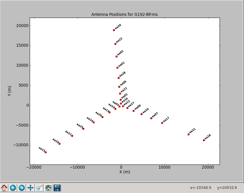
As can be seen (Figure 2), possibly after zooming in with the
magnifying glass icon, for example antenna "ea05" (with ID 3) is
located close to the center. Using the
flagdata
task with mode='summary' it can be seen that "ea05" has a low
percentage of flags. Therefore, this antenna can be used relatively
safely as the reference antenna; for convenience (and for people with
memory issues) introduce a standard descriptive variable name for it:
# In CASA, define the reference antenna identifier using a standard name:
id_ref = 'ea05' (or '3' or 'W08' which are the antenna ID number or pad name for ea05)
3) Setting the Model of the Flux Density Calibrator
To start preparing for a flux comparison later (below, in step C
mentioned above), insert the spectral and angular models for the flux
density calibrator, here 3C147 (field 0), with the
setjy task. Use the 'Perley-Butler 2017' standard and 3C147_A.im for Ka-band (which can be written as id_flx+'_A.im because here fortunately id_flx and the model name agree):
# In CASA, insert the the flux density calibrator model in the MS model column:
setjy(vis=id_ms, field=id_flx, scalebychan=True,
      standard='Perley-Butler 2017', model=id_flx+'_A.im');
- scalebychan=True: If scalebychan=False setjy would use a single value per spectral window.
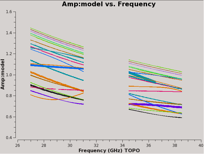
Inspecting the logger report shows that the flux density calibrator (3C147 here) has amplitudes ranging from about 1.0 to about 1.5 Jy across the spws. (Note the output sorting in increasing spw number, not in frequency.)
The model data can be plotted, e.g. for antenna 'ea03', using plotms (Figure 1):
# In CASA, plot the model amplitude as function of frequency
#   for baselines to antenna ea03:
plotms(vis=id_ms, field=id_flx, antenna='ea03',
       xaxis='freq', yaxis='amp', ydatacolumn='model',coloraxis='ant2')
This plot shows baselines to antenna "ea03". Since both a spectral and an angular model for this well resolved calibrator was provided, each baseline has a somewhat different amplitude and phase behavior as function of frequency for baselines to this antenna. Selecting another antenna for the plot will slightly change the curves. Also, a different CASA version or other update (or picking the wrong sourceName_frequencyBand model) would show a different behavior.
A) Calibrating Initial Delays and Bandpass Solutions
Start this entire bandpass calibration procedure with a phase-only, time-dependent (self-)calibration solution for the bandpass calibrator using the parameter gaintype='G' option in gaincal, which should be easy for these supposedly bright sources. Note that the calibration solutions are written to a calibration table, cal.ign, where 'ign' after the standardized calibration table prefix name (cal)stands for per-integration gain. This table is not a variable but a file/directory name in the working directory so it needs to be quoted in the input parameter. Solutions for each integration will remove most of the (phase) decorrelation of the signal allowing for the delay/bandpass calibration to succeed. For best results, the phase variations will be derived from a narrow range of channels near the centers of each spw (say 60~68 here, out of the 128 available per spw), narrow enough to not be affected by uncorrected delay (i.e., reduce possible decorrelation by excluding any large phase differences due to a phase slope over the frequency range of the spw):
# In CASA, do a phase-only self-calibration on the bandpass calibrator
#   (self-calibrating amplitudes is premature before determining a
#   preliminary bandpass calibration and will be done in a later step):
gaincal(vis=id_ms, caltable='cal.ign',
        field=id_bp, spw='*:60~68',
        gaintype='G', refant=id_ref, calmode='p',
        solint='int', minsnr=3)
- refant=id_ref : Use the variable identifying the reference antenna (ea05 here) as the reference antenna.
- solint='int' : Do a per-integration solve (every 6 seconds, which is the time-averaging applied to the data for this tutorial).
- minsnr=3 : Apply a minimum signal-to-noise cutoff of three. Solutions with less signal-to-noise than this value will be flagged.
- gaintable is not set here as earlier calibrations (to prepare for this tutorial have already been applied.
Check that the phase solutions, colored by spw, are smoothly varying,
supposedly reflecting the changing phases due to atmospheric effects
(i.e., for these high frequencies due to the troposphere):
# In CASA, plot phase solutions as function of time, displaying one-for-one
#   a plot for baselines to each antena:
plotms(vis='cal.ign', xaxis='time', yaxis='phase', iteraxis='antenna', coloraxis='spw')
Note that the first plot showing the results for antenna ea01 is empty as ea01 previously was fully flagged, and so were ea10 and ea19. Click on the green arrows to pass through the plots for the other antennas. Also note that the reference antenna (ea05 here) has all phases equal to zero degrees, which they should be by definition for the reference antenna.
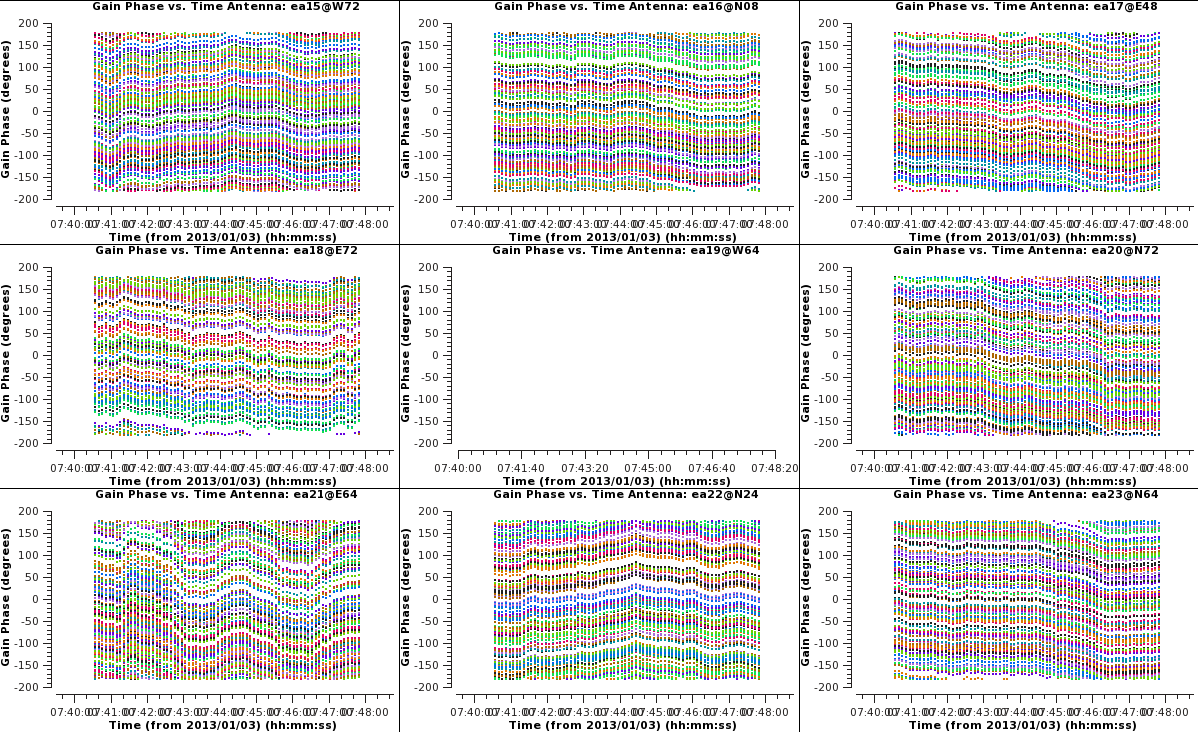
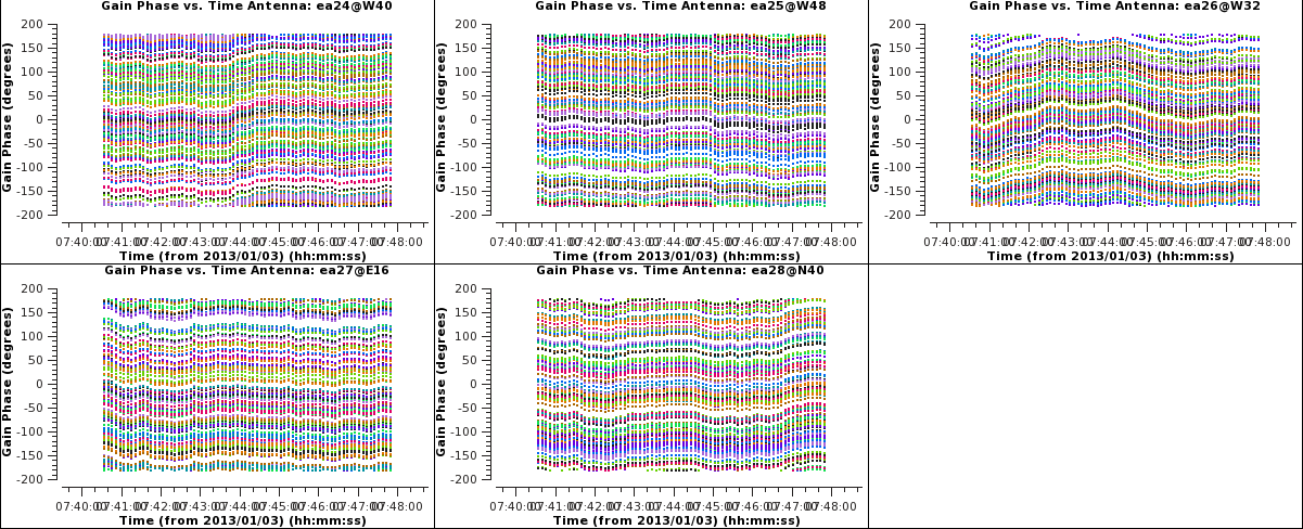
Multipanel plots of the phase solutions can be written to output files as well as to the screen display (Figures 3a, 3b, & 3c). The output files that are generated are in the format of their extention in the plotfile parameter, in this case PNG files, and if the parameter is set to create output in the working directory, can be viewed at any occasion using CASA by executing an external viewer program, e.g., !xv <visbase>_cal.ign_p1*.png; or by running an image viewing application such as xv, Preview, Gimp, Photoshop, etc., external to CASA at the operating system level. Note that the hardcopy only shows the first page, requiring three plotms instances of 3x3 plots to cover all antennas in the MS.
# In CASA, dump images of multi-panel plots for different antenna-ID ranges
#   (antenna-ID 1 to 11, not 1-9 as the antennas with index 7 and 10 are not
#   present as can be noticed in the MS summary <visbase>_list.txt.
#   Unlike anything else in CASA-python indexing, antenna IDs start at one
#   instead of zero):
plotms(vis='cal.ign', xaxis='time', yaxis='phase',
       antenna='1~11', gridrows=3, gridcols=3, iteraxis='antenna',
       coloraxis='spw', plotfile=visbase+'_cal.ign_p1.png')
Note that recently the name of the output file gets appended with the selection of
the iteraxis and there unfortunately seems to be no possibility to switch that off;
to get the file name as specified in the plotfile-parameter one would edit the file
name using the operating system tools.
# second page batch (next nine antennas)
plotms(vis='cal.ign', xaxis='time', yaxis='phase',
       antenna='12~20', gridrows=3, gridcols=3, iteraxis='antenna',
       coloraxis='spw', plotfile=visbase+'_cal.ign_p2.png')

# third page batch (remaining six antennas)
plotms(vis='cal.ign', xaxis='time', yaxis='phase',
       antenna='21~26', gridrows=2, gridcols=3, iteraxis='antenna',
       coloraxis='spw', plotfile=visbase+'_cal.ign_p3.png')
The next step is to solve for the residual delays using the parameter
gaintype='K' option in
gaincal
and store the solutions in the cal.dly table (dly for
delay). Note that this currently does not do a global
fringe-fitting solution for delays. Instead it determines a
baseline-based delay solution per spw for all baselines to the
reference antenna, treating these as antenna-based delays. In most
cases, with high enough S/N to get baseline-based delay solutions,
this will suffice. Avoid the edge channels of each spectral window by
de-selecting them (say, select channels 5~122 here, from the 128
available per spw):
# In CASA, determine residual delays from the bandpass calibrator scans:
gaincal(vis=id_ms, caltable='cal.dly',
        field=id_bp, spw='*:5~122', gaintype='K',
        gaintable=['cal.ign'],
        refant=id_ref, solint='inf', minsnr=3)
Note that this applies the initial phase table cal.ign to reduce decorrelation due to short-term phase fluctuations (as they will be corrected by the solutions in cal.ign).
Alternatively, one can derive a delay across all spws of a baseband. If this is desired, use parameter combine='spw' in gaincal and run the task for each baseband separately (here, in four groups of 16 spw). The solutions from the second and following runs can be appended to the same calibration table via parameter append=True.
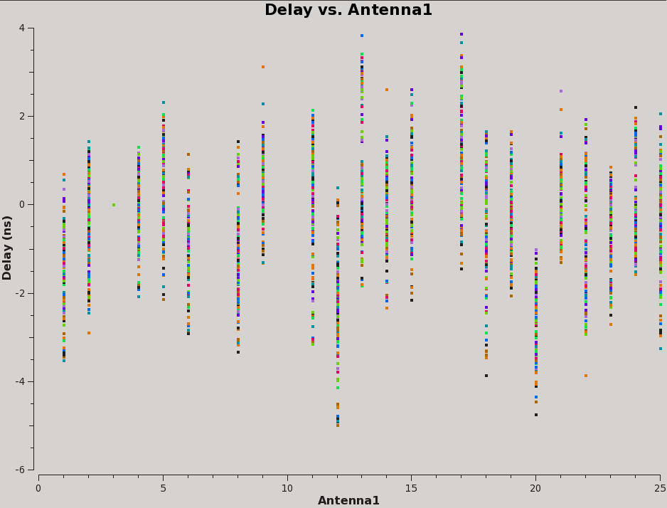
Now plot the delays as a function of antenna index (using one colored dot for each spw and polarization):
# In CASA, display the delay solutions for each spw as function of antenna-ID:
plotms(vis='cal.dly', xaxis='ant1', yaxis='delay', coloraxis='spw')
The delays range from around -5 to 4 nanoseconds (Figure 4).
Now solve for the antenna bandpasses using the previously generated tables cal.ign and cal.dly correcting for possible decorrelation due to phase and delay inaccuracies, and store the solutions in cal.bp (bp for bandpass):
# In CASA, determine the bandpass from the bandpass calibrator scans:
bandpass(vis=id_ms, caltable='cal.bp',
         gaintable=['cal.ign', 'cal.dly'],
         field=id_bp, refant=id_ref, solnorm=False,
         bandtype='B', solint='inf')
WARNING: Set solnorm=False here; otherwise there will be some offsets seen later between spws due to the way the amplitude scaling adjusts weights internally during solving.
Expect to see solutions failing due to "Insufficient unflagged
antennas" — these are for bad channels that have been
pre-flagged.
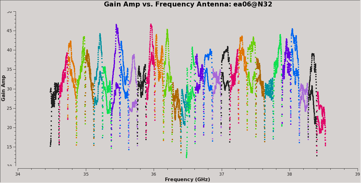
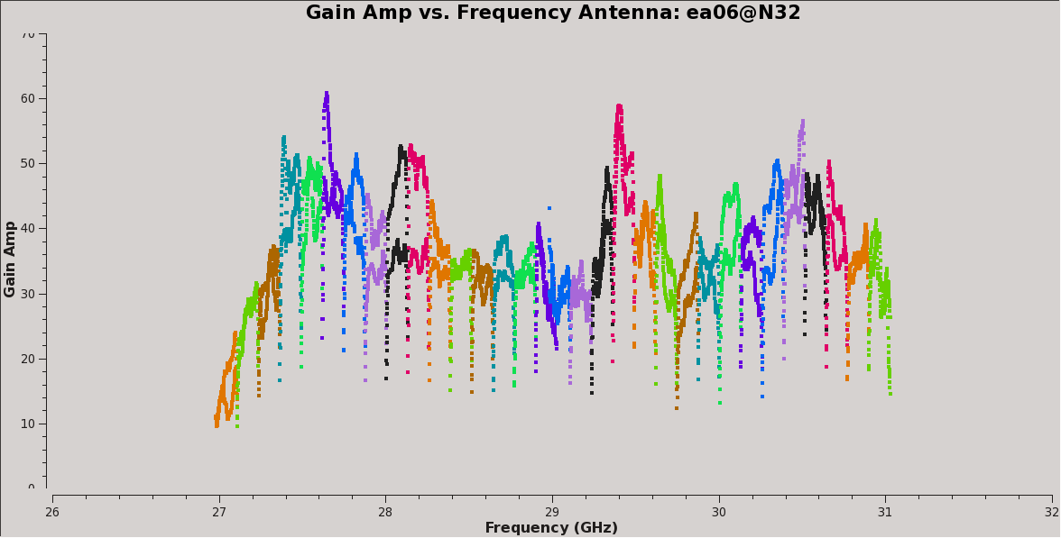
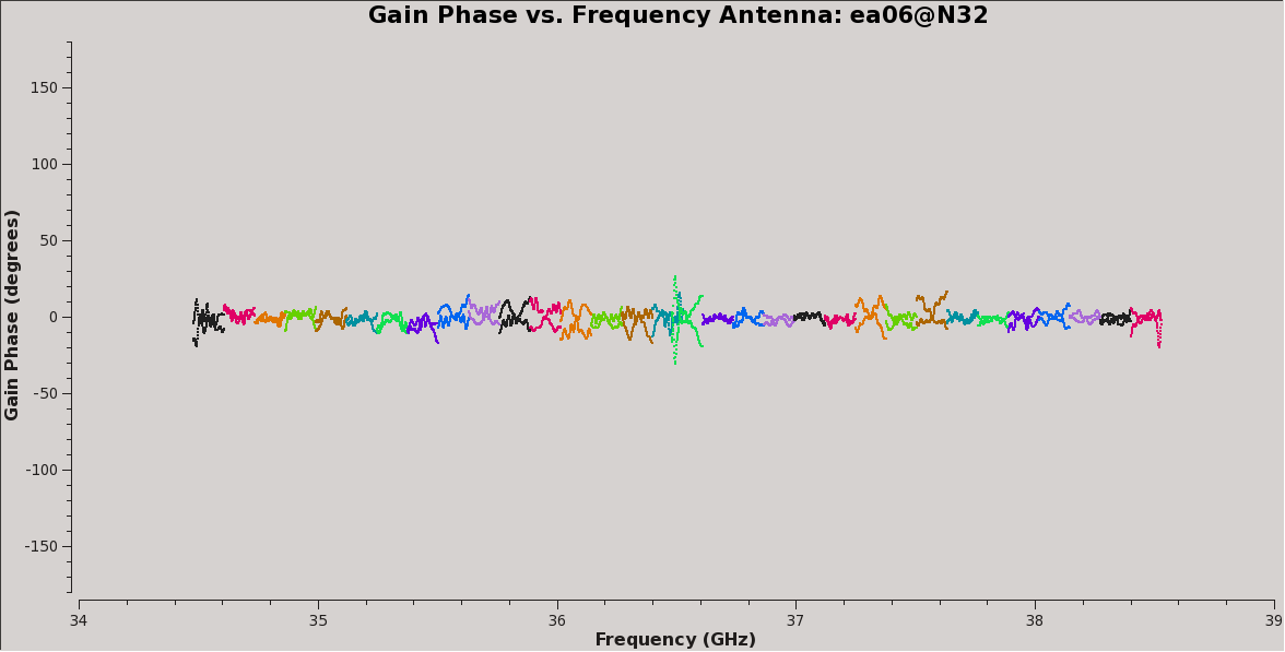
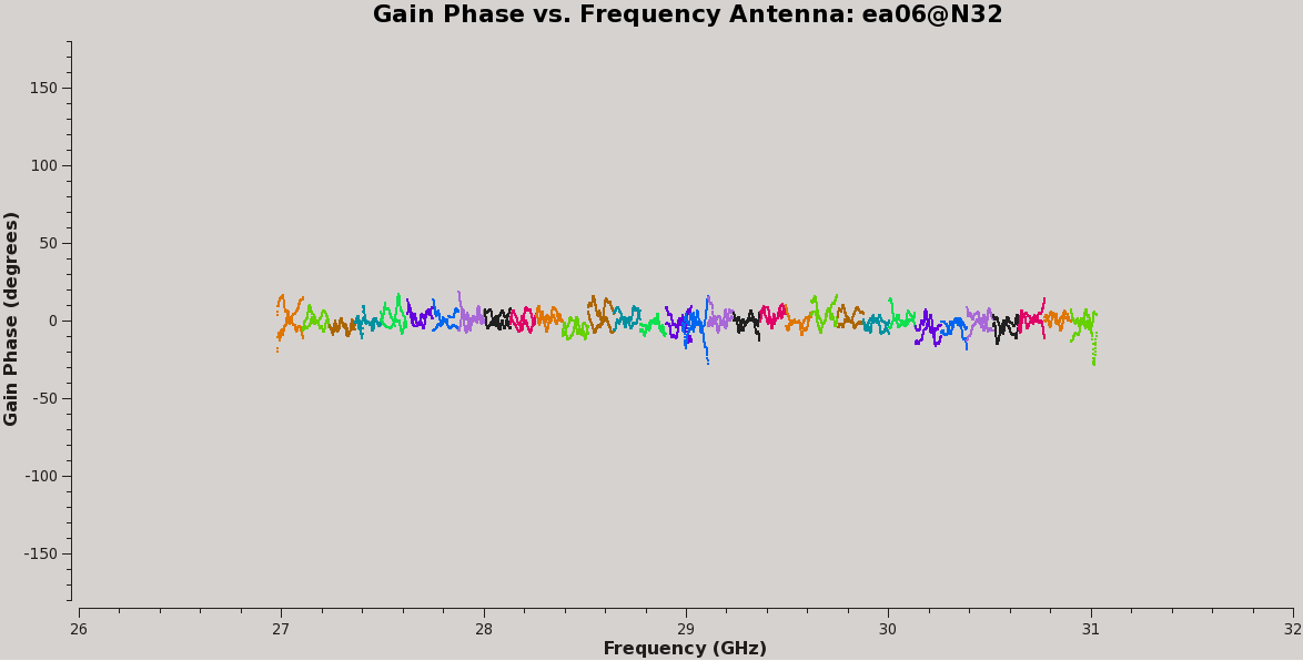
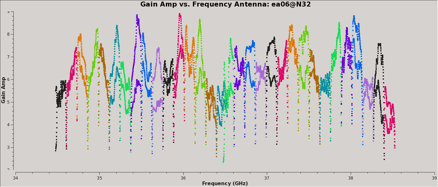
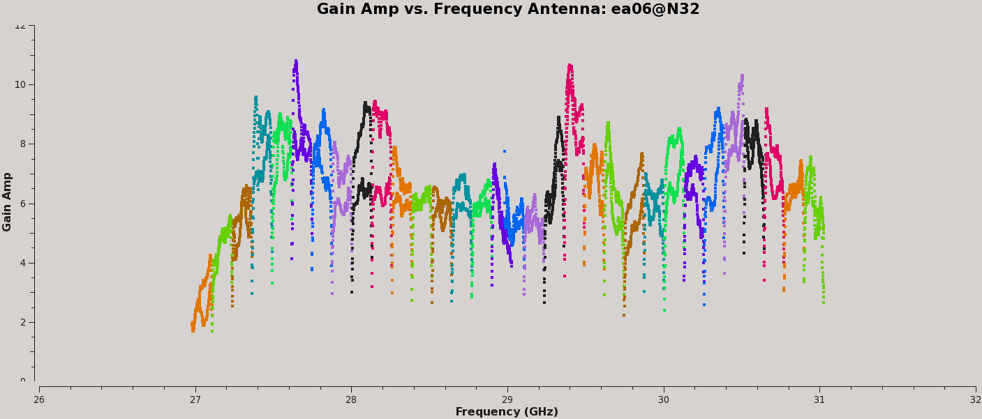
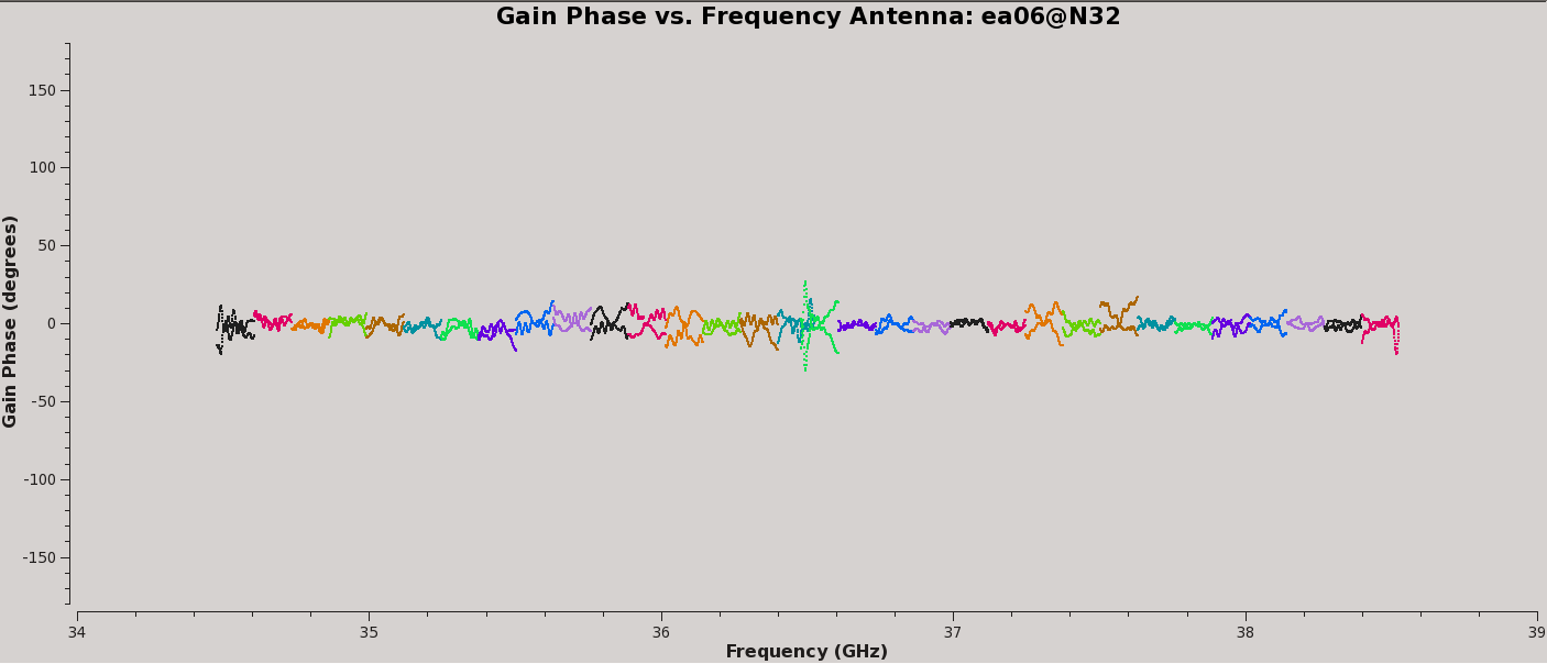
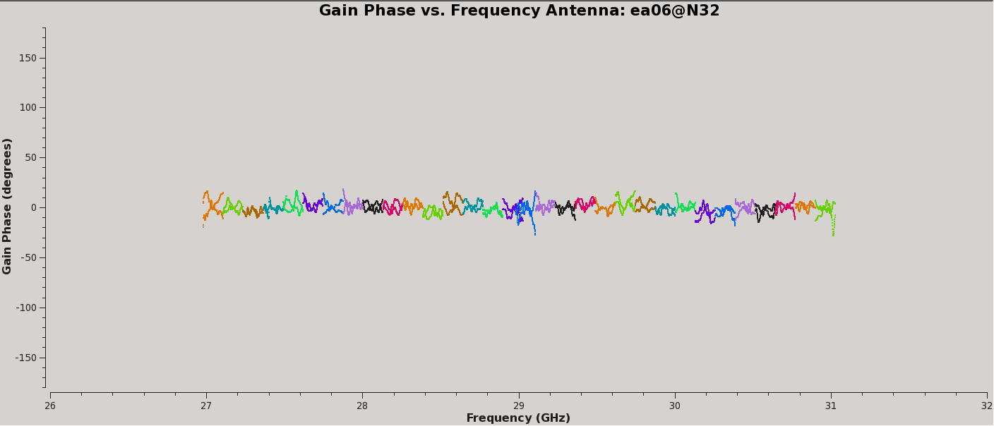
Plot the amplitude and phase soutions of this new bandpass. Note that the first panel with ea01 is empty as it is completely flagged. Proceed to ea06 to see the plots as shown in Figures 5a, 5b, 6a, and 6b:
# In CASA, display the bandpass solutions for amplitude and phase for
#   the different (2x 4GHz) spw ranges; first range, amplitude:
plotms(vis='cal.bp', xaxis='freq', yaxis='amp',
       spw='0~31', iteraxis='antenna', coloraxis='spw')

# second range, amplitude:
plotms(vis='cal.bp', xaxis='freq', yaxis='amp',
       spw='32~63', iteraxis='antenna', coloraxis='spw')

# first range, phase:
plotms(vis='cal.bp', xaxis='freq', yaxis='phase',
       spw='0~31', iteraxis='antenna', coloraxis='spw',
       plotrange=[-1,-1,-80,80])

# second range, phase:
plotms(vis='cal.bp', xaxis='freq', yaxis='phase',
       spw='32~63', iteraxis='antenna', coloraxis='spw',
       plotrange=[-1,-1,-80,80])
B) Applying the Initial Bandpass Solutions to the Flux Density Calibrator
Since there is no a priori spectral information for the chosen bandpass calibrator (here 3C84), bootstrapping it is needed to determine its spectral behavior. This information is then used to re-determine the bandpass in order to avoid folding the intrinsic spectral shape of the bandpass calibrator into the bandpass calibration.
First, repeat the phase-only self-calibration solution with the preliminary determined delay and bandpass calibration in the previous step, A), this time for both the bandpass and the flux density calibrator (which need to be separated by a comma) and store the solutions in cal.ign2pha (use the 2pha to distinguish it as the second stage for phase-only). This will correct for short-term phase decorrelation of the signals. Similarly to avoid decorrelation due to a wide frequency range, use the narrow center channel range (which was channel 60~68):
# In CASA, phase-only self-calibrate the flux density and bandpass calibrators
#   using the obtained first-order bandpass calibration above:
gaincal(vis=id_ms, caltable='cal.ign2pha', field=id_flx+','+id_bp,
        gaintable=['cal.dly', 'cal.bp'],
        gaintype='G', refant=id_ref, calmode='p', solint='int', minsnr=3)
This again allows to calibrate both phase and gain for each scan, now corrected (biased) with the delay and bandpass of the bandpass calibrator. Store the solutions in cal.ign2 (use the 2 to distinguish it as the second pass gain calibration):
# In CASA, now self-calibrate the phase-corrected amplitudes as well:
gaincal(vis=id_ms, caltable='cal.ign2', field=id_flx+','+id_bp,
        gaintable=['cal.dly', 'cal.bp','cal.ign2pha'],
        gaintype='G', refant=id_ref, calmode='ap', solint='inf', minsnr=3)
C) Bootstrapping the Bandpass Calibrator Field Spectrum
With full, phase and amplitude gain solutions for both the flux density and bandpass calibrators, now use fluxscale to scale the gain amplitudes of the bandpass calibrator using those of the flux density calibrator. Store the solutions in cal.bpflx and the flux density results for the bandpass calibrator in <visbase>+'_'+id_bp+'_fluxinfo.txt':
# In CASA, determine the bandpass calibrator fluxes as function of frequency by
#   using the fluxes set for the flux density calibrator with setjy earlier and
#   store the output dictionary with these values in the variable flux_bp:
flux_bp = fluxscale(vis=id_ms, caltable='cal.ign2',
                  fluxtable='cal.bpflx', reference=id_flx, transfer=id_bp,
                  listfile=visbase+'_'+id_bp+'_fluxinfo.txt', fitorder=1)
- flux_bp = fluxscale(...): the python dictionary returned by the fluxscale task will be stored in the flux_bp variable. Inspect the dictionary flux_bp by typing "print flux_bp" at the CASA command line. Alternatively, when not interested in the dictionary type fluxscale(...); with a semicolon after the parentheses and not assigning it to a variable. This will prevent the dictionary to be printed in the terminal. Here however the dictionary is captured in flux_bp as it is going to be used below
- fluxtable='cal.bpflx': this is the output scaled gain table containing the flux density of the bandpass calibrator as function of frequency. Since this is only used to find the spectral index of the bandpass calibrator source field, this table is not used further.
- listfile=visbase+'_'+id_bp+'_fluxinfo.txt': an output file that contains the derived flux values and fit information.
- fitorder=1: only find a (linear) spectral index, ignoring curvature in the spectrum.
- reference=id_flx: the reference field from which the flux scaling is transferred (here: the flux density calibrator 3C147, field 0, assigned by id_flx)
- transfer=id_bp: the target field to which the flux scaling is transferred (here: the bandpass calibrator 3C84, field 1, assigned by id_bp)
The last line in the file (and displayed in the logger) shows, using the default model supplied with this CASA version:
Fitted spectrum for 3c84-J0319+413 with fitorder=1: Flux density = 29.0286 +/- 0.0308709 (freq=32.5128 GHz) spidx=-0.538803 +/- 0.00883078
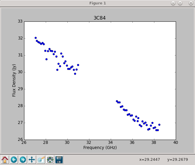
Using the information in the returned flux_bp dictionary, the derived spectrum can be plotted (Figure 7); for that the two loops below fill the parameter variables used in the plotting:
Note that the use of ipython in the command line requires the use of "%cpaste" to allow
copy/pasting of loops, conditions, etc..  Press "Enter" (or "Return") after "--" at the
end. This stops (exits) the copy/paste prompt and will return the CASA command line prompt.
# In CASA, use python code to plot the model spectrum of the bandpass calibrator:

import matplotlib.pyplot as pl
%cpaste

# Press Enter or Return, then copy/paste the following:
freq = flux_bp['freq'] / 1e9
spw_list = range(0,63)
spw_str = []
for i in spw_list:
   thisspw = str(i)
   spw_str.append(thisspw)

bootstrapped_fluxes = []
for j in spw_str:
    thisflux = flux_bp['1'][j]['fluxd'][0]
    if thisflux == None:
        continue
    else:
        bootstrapped_fluxes.append(thisflux)

pl.clf()
pl.plot(freq, bootstrapped_fluxes, 'bo')
pl.xlabel('Frequency (GHz)')
pl.ylabel('Flux Density (Jy)')
pl.title(id_bp)
pl.show()
--
The model from fluxscale is used to fill the MODEL column with the bandpass source's spectral information using setjy. With standard='fluxscale' , we can directly use the flux_bp python dictionary as input via fluxdict:
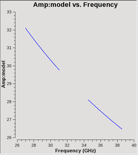
# In CASA, insert the spectral information for the bandpass calibrator field:
setjy(vis=id_ms, field=id_bp, scalebychan=True,
      standard = 'fluxscale', fluxdict=flux_bp);
Check with plotms that the data have been appropriately filled (Figure 8):
# In CASA, display the spectral model of the bandpass calibrator field, in this
#   case for a specific baseline (which should be identical for all baselines
#   for a point-like source, otherwise it will depend on baseline length):
plotms(vis=id_ms, field=id_bp, antenna='ea05&ea02',
       xaxis='freq', yaxis='amp', ydatacolumn='model')
D) Creating a New Bandpass using the Bandpass Calibrator Spectral Model
Next, redo the previous calibration using this new model information as if it were a standard flux density calibrator. Although the commands are the same as issued earlier, keep in mind that the model values for the bandpass calibrator have changed and, therefore, the results of these calibration calculations accordingly will differ if the specral index differs significanlty from the spectral index of the flux density calibrator:
# In CASA, redo a phase-only self-calibration on the bandpass calibrator:
gaincal(vis=id_ms, caltable='cal.ign.redo',
        field=id_bp, spw='*:60~68',
        gaintype='G', refant=id_ref, calmode='p',
        solint='int', minsnr=3)

# In CASA, re-determine residual delays from the bandpass calibrator scans:
gaincal(vis=id_ms, caltable='cal.dly.redo',
        gaintable=['cal.ign.redo'],
        field=id_bp, spw='*:5~122', gaintype='K',
        refant=id_ref, solint='inf', minsnr=3)

# In CASA, re-determine the bandpass from the bandpass calibrator scans:
bandpass(vis=id_ms, caltable='cal.bp.redo',
         gaintable=['cal.ign.redo', 'cal.dly.redo'],
         field=id_bp, refant=id_ref, solnorm=False,
         bandtype='B', solint='inf')
Finally, inspect these solutions (Figures 9a, 9b, 10a, and 10b; again note that antenna ea01 is fully flagged):
# In CASA, display and check the bandpass solutions; first range, amplitude:
plotms(vis='cal.bp.redo', xaxis='freq', yaxis='amp',
       spw='0~31', iteraxis='antenna', coloraxis='spw')

# second range, amplitude:
plotms(vis='cal.bp.redo', xaxis='freq', yaxis='amp',
       spw='32~63', iteraxis='antenna', coloraxis='spw')

# first range, phase:
plotms(vis='cal.bp.redo', xaxis='freq', yaxis='phase',
       spw='0~31', iteraxis='antenna', coloraxis='spw',
       plotrange=[-1,-1,-180,180])

# second range, phase:
plotms(vis='cal.bp.redo', xaxis='freq', yaxis='phase',
       spw='32~63', iteraxis='antenna', coloraxis='spw',
       plotrange=[-1,-1,-180,180])
As in this particualr observation the spectral indices for the flux density calibrator (3C147: -0.696, standard) and the bandpass calibrator (3C84: -0.626, derived here) are very similar, the solutions look virtually unchanged from the previous solutions with the exception that the amplitude scaling is corrected for the spectrum of the bandpass calibrator. These steps yielded the final version of the delay and bandpass calibration tables, cal.dly.redo and cal.bp.redo, which now would be used for all subsequent calibration steps.
Last checked on CASA Version 6.4.1
Cheat Sheet - all commands summarized
(Note that the automatic formatting here may introduce some weirdness in displaying the pre-formatted text and single line commands; be aware when copy/pasting that the line is complete, i.e., ending with the closing parenthesis and/or semicolon.)
# in a terminal, outside of CASA
tar -xzf G192-BP.ms.tar.gz
casa -r 6.4.1-12-pipeline-2022.2.0.64

# inside of CASA, CASA command line
visbase='G192-BP'
id_ms=visbase+'.ms'
  listobs(vis=id_ms,listfile=visbase+'_list.txt');
id_flx='3C147'
id_bp='3c84-J0319+413'
  plotants(vis=id_ms,antindex=True,logpos=True)
id_ref='ea05'
setjy(vis=id_ms,field=id_flx,scalebychan=True,standard='Perley-Butler 2017',model=id_flx+'_A.im');
  plotms(vis=id_ms,field=id_flx,antenna='ea03',xaxis='freq',yaxis='amp',ydatacolumn='model',coloraxis='ant2')

# Step A) ---
gaincal(vis=id_ms,caltable='cal.ign',field=id_bp,spw='*:60~68',gaintype='G',refant=id_ref,calmode='p',solint='int',minsnr=3)
  plotms(vis='cal.ign',xaxis='time',yaxis='phase',iteraxis='antenna',coloraxis='spw')
  plotms(vis='cal.ign',xaxis='time',yaxis='phase',antenna='1~11',gridrows=3,gridcols=3,iteraxis='antenna',coloraxis='spw',plotfile=visbase+'_cal.ign_p1.png')
  plotms(vis='cal.ign',xaxis='time',yaxis='phase',antenna='12~20',gridrows=3,gridcols=3,iteraxis='antenna',coloraxis='spw',plotfile=visbase+'_cal.ign_p2.png')
  plotms(vis='cal.ign',xaxis='time',yaxis='phase',antenna='21~26',gridrows=2,gridcols=3,iteraxis='antenna',coloraxis='spw',plotfile=visbase+'_cal.ign_p3.png')
gaincal(vis=id_ms,caltable='cal.dly',field=id_bp,spw='*:5~122',gaintype='K',gaintable=['cal.ign'],refant=id_ref,solint='inf',minsnr=3)
  plotms(vis='cal.dly',xaxis='ant1',yaxis='delay',coloraxis='spw')
bandpass(vis=id_ms,caltable='cal.bp',gaintable=['cal.ign','cal.dly'],field=id_bp,refant=id_ref,solnorm=False,bandtype='B',solint='inf')
  plotms(vis='cal.bp',xaxis='freq',yaxis='amp',spw='0~31',iteraxis='antenna',coloraxis='spw',plotrange=[-1,-1,0,80])
  plotms(vis='cal.bp',xaxis='freq',yaxis='amp',spw='32~63',iteraxis='antenna',coloraxis='spw',plotrange=[-1,-1,0,80])
  plotms(vis='cal.bp',xaxis='freq',yaxis='phase',spw='0~31',iteraxis='antenna',coloraxis='spw',plotrange=[-1,-1,-80,80])
  plotms(vis='cal.bp',xaxis='freq',yaxis='phase',spw='32~63',iteraxis='antenna',coloraxis='spw',plotrange=[-1,-1,-80,80])

# Step B) ---
gaincal(vis=id_ms,caltable='cal.ign2pha',field=id_flx+','+id_bp,gaintable=['cal.dly','cal.bp'],gaintype='G',refant=id_ref,calmode='p',solint='int',minsnr=3)
gaincal(vis=id_ms,caltable='cal.ign2',field=id_flx+','+id_bp,gaintable['cal.dly','cal.bp','cal.ign2pha'],gaintype='G',refant=id_ref,calmode='ap',solint='inf',minsnr=3)

# Step C) ---
flux_bp=fluxscale(vis=id_ms,caltable='cal.ign2',fluxtable='cal.bpflx',reference=id_flx,transfer=id_bp,listfile=visbase+'_'+id_bp+'_fluxinfo.txt',fitorder=1)

import matplotlib.pyplot as pl
%cpaste

freq = flux_bp['freq'] / 1e9
spw_list = range(0,64)
spw_str = []
for i in spw_list:
   thisspw = str(i)
   spw_str.append(thisspw)
bootstrapped_fluxes = []
for j in spw_str:
    thisflux = flux_bp['1'][j]['fluxd'][0]
    if thisflux ==None:
        continue
    else:
        bootstrapped_fluxes.append(thisflux)
pl.clf()
pl.plot(freq,bootstrapped_fluxes,'bo')
pl.xlabel('Frequency (GHz)')
pl.ylabel('Flux Density (Jy)')
pl.title(id_bp)
pl.show()
--

setjy(vis=id_ms,field=id_bp,scalebychan=True,standard='fluxscale',fluxdict=flux_bp);
  plotms(vis=id_ms,field=id_bp,antenna='ea05&ea02',xaxis='freq',yaxis='amp',ydatacolumn='model')

# Step D) ---
gaincal(vis=id_ms,caltable='cal.ign.redo',field=id_bp,spw='*:60~68',gaintype='G',refant=id_ref,calmode='p',solint='int',minsnr=3)
gaincal(vis=id_ms,caltable='cal.dly.redo',gaintable=['cal.ign.redo'],field=id_bp,spw='*:5~122',gaintype='K',refant=id_ref,solint='inf',minsnr=3)
bandpass(vis=id_ms,caltable='cal.bp.redo',gaintable=['cal.ign.redo','cal.dly.redo'],field=id_bp,refant=id_ref,solnorm=False,bandtype='B',solint='inf')
  plotms(vis='cal.bp.redo',xaxis='freq',yaxis='amp',spw='0~31',iteraxis='antenna',coloraxis='spw',plotrange=[-1,-1,0,15])
  plotms(vis='cal.bp.redo',xaxis='freq',yaxis='amp',spw='32~63',iteraxis='antenna',coloraxis='spw',plotrange=[-1,-1,0,15])
  plotms(vis='cal.bp.redo',xaxis='freq',yaxis='phase',spw='0~31',iteraxis='antenna',coloraxis='spw',plotrange=[-1,-1,-80,80])
  plotms(vis='cal.bp.redo',xaxis='freq',yaxis='phase',spw='32~63',iteraxis='antenna',coloraxis='spw',plotrange=[-1,-1,-80,80])

