Calibrating M99

↵ CARMA Tutorials

This tutorial assumes you have converted your data from native MIRIAD format to a CASA measurement set (MS); in particular, this example uses the CARMA STING dataset imported in the tutorial Importing M99. It also assumes that you have put the filename of the original MS into a global CASA variable, e.g.,

# In CASA
msdir='./'
project='c0104I'
msfile=msdir+project+'.ms'

Note: This tutorial details a particular calibration path optimized for the example dataset being used; in cases where alternatives command calls are described, these commands are commented out. The intention is that they will then be extracted with all other commands in this tutorial, and you can uncomment them if you wish to try them. See Extracting scripts from these tutorials for more information.

Examining your data

The beginning of the output from listobs.

The end of the output from listobs.

plotants output showing antenna positions.

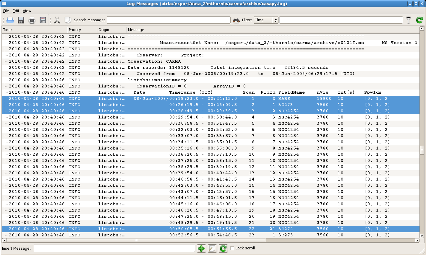
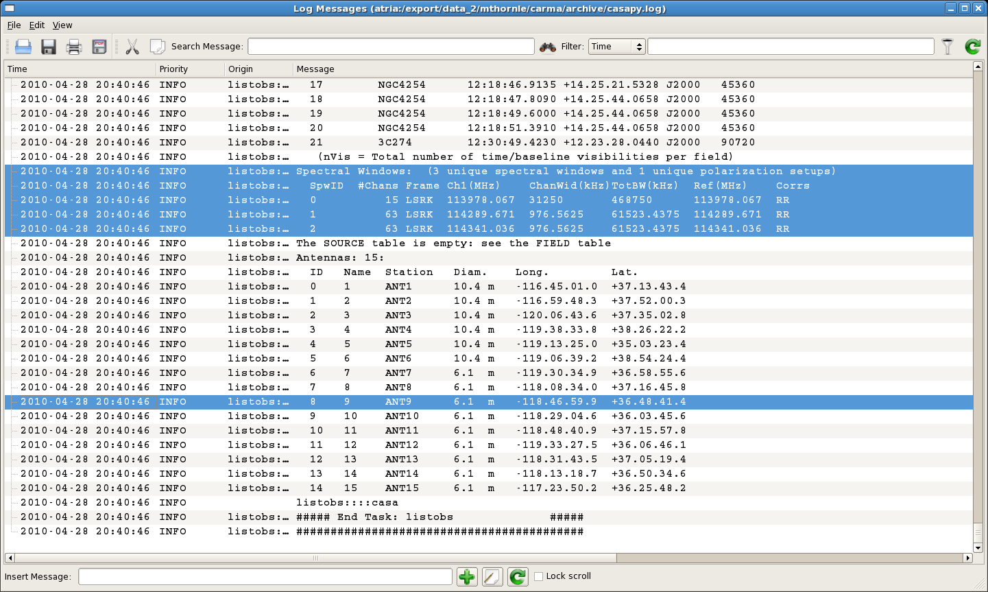
You'll need some information about the IDs that CASA assigns to your calibrators, sources, and antennas. So if you haven't yet done so,

# In CASA
listobs(vis=msfile)

You will want to look through the listobs output to determine:

• The Field ID (FldId) or source name (as listed in the header) of each of your sources and calibrators.
• The Spectral Window ID (SpwID) of each spectral window you want to calibrate.
• The Name (or station; the ID number is actually least useful) of your reference antenna.

Near the beginning of the listobs output, you will find the first listing of FldId numbers. In this example, the flux calibrator (MARS) is assigned FldId=0, the bandpass (and phase) calibrator (3C273) is assigned FldId=1, the mosaicked source fields are assigned FldId 2 through 20 (that's field='2~20' in python), and an extra "test" calibrator was also observed (3C274) and assigned FldId=21. Any "field=" input can be filled with either the object's Field ID or source name.

Near the end of the listobs output, you will find listings of the properties of the observed spectral windows, and the locations of the antennas. In this case, the narrowband windows are assigned to SpwID of 1 and 2, and they each have 63 channels. The reference antenna is Antenna 9, which unfortunately here is named '9'. For unambiguous antenna selection, ideally the Name (which CASA searches first) should have text in it; if it does not, you may want to use the unambiguous Station name of 'ANT9' to ensure that CASA chooses the right antenna.

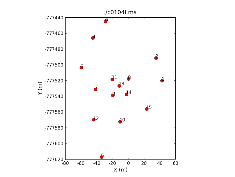
If you'd prefer a graphical representation of antenna positions in order to choose your reference antenna, you can use plotants. The following command

# In CASA
plotants(vis=msfile,figfile='plotants.png')

will display the physical layout of the antennas.You can see antenna 9 near the middle of the CARMA antenna distribution.

Beta-alert: At the time of this revision (CASA 3.2), plotants was leaving table.lock files that make the rest of the tutorial unhappy. Here's a pythonic way to zap those table.lock files.

import os
for root, dirs, files in os.walk('./'):
    for name in files:
        if name == 'table.lock': os.remove(os.path.join(root,name))

Calibrating your data

Before running your calibration, it's a good idea to run the following command:

# In CASA
clearcal(vis=msfile)

If this is the first time you've calibrated, clearcal won't do much, but it will initialize table columns that might be missing from the import step (you may see some output to the log screen to this effect). If you are trying a new calibration, this command ensures your data returns to their original state. So it can't hurt you, and can help.

Calibration in CASA consists of creating calibration tables, and then applying them as needed. Here, we step you through bandpass and amplitude calibration, and then indicate how to apply them to your source data.

Bandpass calibration

The following command (bandpass) will create a bandpass calibration table (caltable=) using the specified bandpass calibrator (field=FldId) and reference antenna (refant), in the same directory as the data are found. No prior gain tables are applied in this step, but they could be if it were necessary (just fill in the appropriate information for gaintable and gainfield).

# In CASA
default('bandpass')
bandpass(vis=msfile,caltable=msdir+project+'.bcal',gaintable='',gainfield='',
         interp='',field='1',spw='',gaincurve=False,
         bandtype='B',solint='inf',refant='ANT9',
         solnorm=True)

Plotcal GUI showing the bandpass solutions for some of the antennas.

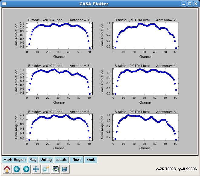
You can look at the bandpass calibration table you've created using plotcal. This first call will plot the *.bcal table to a GUI for you to look at and interact with--here, you are looking at one of the narrowband spectral windows (spw='1'), and making a 3x2 display of bandpass plots, one for each antenna:

# In CASA
plotcal(caltable=msdir+project+'.bcal',xaxis='chan',yaxis='amp',
        iteration='antenna',subplot=321,spw='1',
        showgui=T)

This second call outputs the same kind of plot to a PNG file (filename specified by 'figfile') without opening the interactive GUI:

# In CASA
plotcal(caltable=msdir+project+'.bcal',xaxis='chan',yaxis='amp',
        iteration='antenna',subplot=321,spw='1',
        showgui=F,figfile='bp_spw1')

Amplitude calibration

3C273 was used as a phase calibrator for this observation, but it is strong enough to serve as bandpass and flux calibrator as well, so we will use it for all aspects of calibration in this example. As in AIPS the task setjy is used to provide source information for objects of known flux and distribution. You can use the CARMA flux calibrator database to determine the flux of your flux calibrator at the time of your observation. For these observations, the flux of 3C273 was recorded as 17.8 Jy. You can provide this information to CASA using the following command:

# In CASA
setjy(vis=msfile, field='3C273',fluxdensity=[17.8,0.,0.,0.], spw='0~2')

If you want to use 3C274 as a calibrator as well, you can run setjy on it as well. 3C274 is weaker, at about 3.0 Jy:

# In CASA
setjy(vis=msfile, field='3C274',fluxdensity=[3.0,0.,0.,0.], spw='0~2')

The task gaincal can then be used to determine the appropriate gains to be applied as a function of time. 3C273 is a nice strong calibrator, so we can determine the gain calibration with time for each spw individually. (If there is no amplitude or phase offset between the wide and narrow spw's, you could also use the wideband spw and apply it to each narrowband spw; this may be valuable in the case of a weaker calibrator.) As before, and we have used the station title of the reference antenna (refant='ANT9') to unambiguously identify it.

The bandpass calibration table, specified here by gaintable, is accounted for prior to determining the gain table, so that the two calibrations remain separate. Note: neither the gain or bandpass calibration is actually applied to the source data here; both calibrations will need to be applied after they have been determined, using applycal (see below).

# In CASA
gaincal(vis=msfile,caltable=msdir+project+'.gcal',gaintable=msdir+project+'.bcal',
        gainfield='3C273', field='3C273', spw='', 
        gaintype='G',minsnr=2.0, refant='ANT9', solint='inf', combine='')

plotcal output showing gain calibration for some antennas.

Note: To use only the wideband spw for all gain calibration, you would set spw='0' for this dataset.

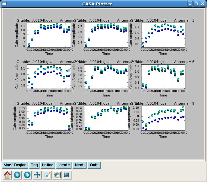
As before with the bandpass calibration table, you can see what the gain calibration table looks like with plotcal (in this example, using the phase calibrator, field='2'):

# In CASA
plotcal(caltable=msdir+project+'.gcal', yaxis='amp',field='3C273',
        iteration='antenna',subplot=331,
        showgui=T)

Now that the gains have been determined, you can bootstrap the flux of 3C273 to the other sources, using fluxscale. This command uses the gain table (specified by caltable) and needs to be told which source has a known flux (reference=). In this example, we are also using 3C273 as the phase calibrator, so fluxcal is not needed, but if we wanted to use 3C274 as a calibrator as well we would need to transfer fluxes over using fluxscale. (Note: if there are no other calibrators in your file, CASA will complain and this call to fluxscale will likely cause your script to stop.)

# In CASA
# needed if your phase calibrator is distinct from your flux calibrator
fluxscale(vis=msfile,caltable=msdir+project+'.gcal',
          fluxtable=msdir+project+'.fcal', reference='3C273')

Note: All of the information from the gain table is contained in the flux table, so in the end, you will apply the bandpass and flux calibration tables in order to apply all relevant calibrations to your source data.

Applying your calibrations

Now that you have solutions for both bandpass and gain calibration, you can apply them to your data. Note that applycal does not operate on the raw data in this step, so you do not need to create a copy of the data before proceeding. Use of the command clearcal will return your data to a pristine state, if needed.

Applycal is fairly flexible, allowing you to apply multiple calibration tables, and calibrations from one spectral window to others (however, you may need to consider the task accum if you have multiple pairs of sources and calibrators in the same dataset; see section 4.3 ('Apply the calibrations') of Calibrating a VLA 5 GHz continuum survey for an example using VLA data).

Here are two examples of applying calibrations, but these are still relatively simple. Consult the helpfile for applycal for a detailed explanation of how to use this command--note in particular the use of the parameter spwmap.

In the first example, we apply calibrations to the bandpass/flux/phase calibrator (field='3C273', or field='1'). We apply both bandpass and flux calibration tables. The order of entries in gainfield and spwmap are the same as for gaintable: in this case, it means that we take the bandpass calibration for 3C273 (gainfield=['3C273',...) and apply the solutions for each spectral window to the same spectral window for the other sources (spwmap=[[],...), and we do the same for the gain/flux calibration (gainfield=...,'3C273'],spwmap-...,[]]). If you had determined the gain/flux calibration using the wideband channel only (spw='0'), you would apply that calibration to all spectral windows by fixing the second term of spwmap (spwmap=...,[0]]).

You would only want to do this first example if you wanted to image the bandpass/flux/phase calibrator 3C273.

# In CASA
# Apply 3C273 calibrations to itself if you want to image 3C273
applycal(vis=msfile,field='3C273',spw='',  
         gaintable=[msdir+project+'.bcal',msdir+project+'.fcal'],
         gainfield=['3C273','3C273'],spwmap=[[],[0]])

In this second example, we apply bandpass and flux calibrations to the rest of the observed objects (phase calibrator, field='2'; source, field='3~51'). In this case, we use the gain/flux calibration information for the phase calibrator to apply to the source, as it has finer time sampling.

# In CASA
applycal(vis=msfile,field='2~20',spw='',  
         gaintable=[msdir+project+'.bcal',msdir+project+'.fcal'],
         gainfield=['1','2'],spwmap=[[],[0]])

Calibration is now complete! Proceed onward to Imaging a Mosaicked Spectral Line Dataset.

↵ CARMA Tutorials
↵ CASAguides

--Michele Thornley, 28 December 2009