Self-Calibration Template CASA 6.1.1

This guide continues with products created in Image the Continuum Template. All imaging parameters are set in the previous guide. You will need calibrated_final_cont.ms to proceed. Commands for this guide can be found in scriptForImaging_template.py available on github.

Self-Calibration on the Continuum (optional)

If you have a high signal-to-noise detection of your source, you can use the source itself to calibrate the phases and potentially the amplitudes of the visibilities as a function of time. This technique is called self-calibration and takes advantage of the fact that interferometer data is over-constrained (we have more equations than we have solutions). The recommended signal to noise depends on the number of antennas. As a rule of thumb, [xxx add some recommendations here based on Crystal's self-cal presentation].

Self-calibration is an iterative process. You start by generating a model of your source using clean. Then you use this model to determine the gains as a function of time using the gaincal task. Finally you apply these solutions to the data and re-image. These steps are repeated until you are happy with your model or you run out of signal-to-noise. In general, you start with phase-only self-calibration and only do amplitude calibration at the end of the self-calibration process if there are amplitude-based gain artifacts in the data (see the Imaging and Deconvolution talk from the Synthesis Imaging Summer School for more detail. Amplitude calibration should be used with caution because it has the potential to change the fluxes of sources in your data.

Self-calibration can either be performed with line or continuum data. Here we demonstrate how to do it with continuum data. The principle is the same for line data, except you form your image using the brightest line emission. For an example of self-calibration with line data, see the VLA high frequency spectral line tutorial for IRC+10216.

For a more detailed explanation of self-calibration, please see the NRAO Live! presentation When, why, and how to do self-calibration.

---

The first thing you should do when beginning self-calibration is to save the original flags in your data set. This step is necessary because when you apply the calibration to a data set it flags data that is not associated with a solution. Applying a bad calibration table to your data can result in the excessive flagging of your data. Saving your original flags allows you to restore the original state of your data easily.

# in CASA
flagmanager(vis=contvis,mode='save',versionname='before_selfcal',merge='replace')

Now we can set up the parameters for the self calibration. Begin by setting the parameters for your ms and continuum image name. The ms calibrated_final_cont.ms was created in the previous part of this guide: Image the Continuum Template.

# in CASA
contvis = 'calibrated_final_cont.ms'         
contimagename = 'calibrated_final_cont'

If you run the self-calibration process more than once, you will need to remove any models that could be left in the image header; which can be accomplished by using the delmod task as well as the clearcal task (which will need to be uncommented in the code below).

# in CASA
# delmod(vis=contvis,field=field,otf=True)
# clearcal(vis=contvis)

You should use the same reference antenna that was used during calibration. For pipeline reductions, this can be found in the stage hif_refant. For manual reductions, the reference antenna will be stated near the top of *.ms.scriptForCalibration.py. If there are multiple executions, make sure to use an antenna that has good solutions and is present in all executions. The Analysis Utilities task au.commonAntennas can help you find antennas that meet this criteria. If you haven't installed Analysis Utilities, see Obtaining Analysis Utilities for instructions. Tasks such as plotants or listobs/vishead can also be used to find antennas in all executions.

# in CASA
refant = 'DV09' # pick a reference antenna.

In the example below, we combine the signal from all spectral windows to improve the signal-to-noise for our gain solution. When combining the spectral windows, you need to map the solution from the combined spectral window (0) to the individual spectral windows using the spwmap parameter. This parameter is a list where the index of the element in the list indicates the spectral window and the value for that index the window that it is mapped to. For example, if we have three spectral windows in the original data set and use combine='spw' for our gain solution, we set spwmap=[0,0,0] to map spw=0 to spw=0, spw=1 to spw=0, and spw=2 to spw=0.

spwmap = [0,0,0] # mapping self-calibration solutions to individual spectral windows. Generally an array of n zeroes, where n is the number of spectral windows in the data sets.

You then begin the process of shallowly cleaning your continuum data to create an initial model for your data in the model column of your data set. Usually you only should do at most a few hundred iterations on the brightest source(s) in the field.

# in CASA
# shallow clean on the continuum

for ext in ['.flux','.image','.mask','.model','.pbcor','.psf','.residual','.flux.pbcoverage']:
    rmtables(contimagename + '_p0'+ ext)
    
clean(vis=contvis,
      imagename=contimagename + '_p0',
      field=field,
#      phasecenter=phasecenter, # uncomment if mosaic.      
      mode='mfs',
      psfmode='clark',
      imsize = imsize,
      cell= cell,
      weighting = weighting,
      robust=robust,
      niter=niter,
      threshold=threshold,
      interactive=True,
      usescratch=True, # needed for 4.3 and 4.4 (and maybe 4.5)
      imagermode=imagermode)

# Note number of iterations performed.

Next you take that model and use it to determine the per-antenna phase solutions as a function of time using gaincal. We use the rmtables command here to completely eradicate any previous solution table from CASA's memory. Note that we start here with a fairly long solution interval that is the length of a scan (solint='inf').

# per scan solution
rmtables('pcal1')
gaincal(vis=contvis,
        caltable='pcal1',
        field=field,
        gaintype='T',
        refant=refant,
        calmode='p',
        combine='spw',
        solint='inf',
        minsnr=3.0,
        minblperant=6)

Inspect the logging messages output by gaincal to see how many solutions were expected/attempted/succeeded. If you have a large number of failed solutions, do not proceed further! This usually means that you do not have enough signal-to-noise on your source to proceed with self-calibration. Note that if you apply a calibration table with many failed solutions to the data, it will flag the data associated with these solutions. You may try changing the minsnr and minblperant parameters in the gaincal call above to find more solutions, but this option should be used with caution because these parameters are already low.

Calibration solve statistics per spw: (expected/attempted/succeeded):
   Spw 0: 235/235/235
   Spw 1: 235/235/235
   Spw 2: 235/235/235

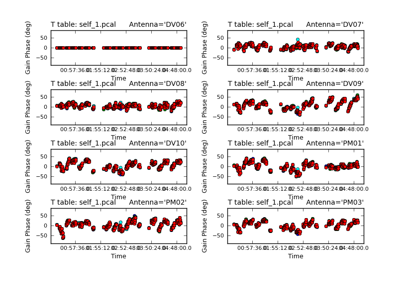
<figure id="Plotcal_image.png">

Figure 1: Solutions from the first round of self-cal.

</figure>

You should also check the solutions (above) that were obtained using plotcal. The solutions should vary smoothly with time and there should not be any large outliers.

In CASA
# Check the solution
plotcal(caltable='pcal1',
        xaxis='time',
        yaxis='phase',
        timerange='',
        iteration='antenna',
        subplot=421,
        plotrange=[0,0,-180,180])

If you are satisfied with the solutions, apply them to the ms. Note: this step usually takes a while, so go ahead and get a cup of coffee.

<figure id="Pcal1.png">

Continuum image after the first round of self-cal.

</figure>

# in CASA
# apply the calibration to the data for next round of imaging
applycal(vis=contvis,
         field=field,
         spwmap=spwmap,
         gaintable=['pcal1'],
         gainfield='',
         calwt=False,
         flagbackup=False,
         interp='linearperobs')

Using our new gain solutions, we can generate an improved model for our source using clean. During this second clean iteration, you should clean a bit deeper than previously, but not all the way down to the noise. Remember the goal here is to build up a good model for your source, so you don't want to include things that are not real emission.

# clean deeper
for ext in ['.flux','.image','.mask','.model','.pbcor','.psf','.residual','.flux.pbcoverage']:
    rmtables(contimagename + '_p1'+ ext)

clean(vis=contvis,
      field=field,
#      phasecenter=phasecenter, # uncomment if mosaic.      
      imagename=contimagename + '_p1',
      mode='mfs',
      psfmode='clark',
      imsize = imsize,
      cell= cell,
      weighting = weighting,
      robust=robust,
      niter=niter,
      threshold=threshold,
      interactive=True,
      usescratch=True, # needed for 4.3 and 4.4 (and maybe 4.5)
      imagermode=imagermode)

# Note number of iterations performed.

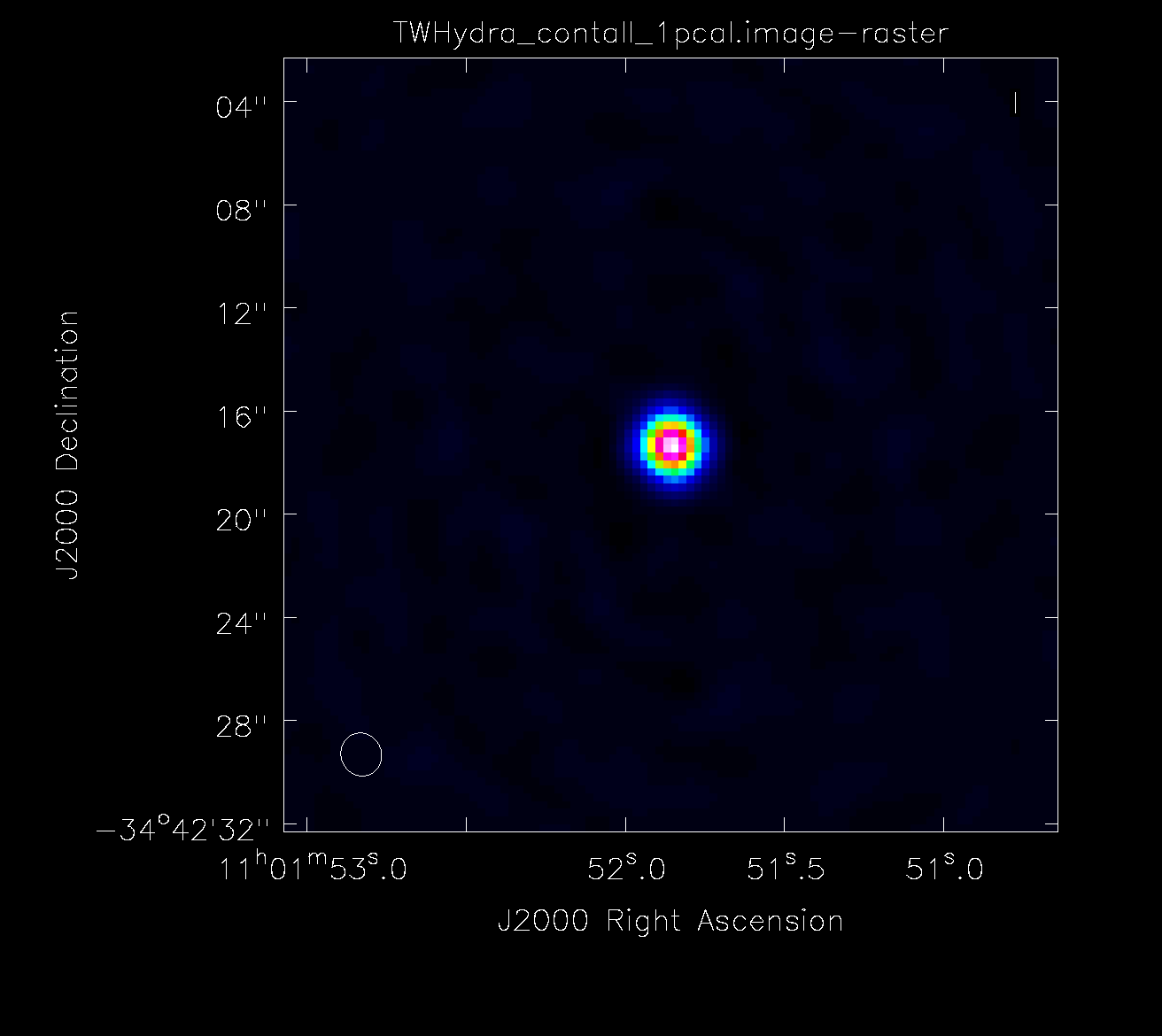
You should inspect the new image in the viewer to assess how well self-calibration worked. In general, the noise should be lower and the signal-to-noise ratio higher than in the original image and there should be no major new artifacts in the image. If the signal-to-noise ratio does not increase, you may not have enough signal-to-noise on your target to run self-calibration. If you don't see an improvement in the image, clear the calibration with clearcal (see commands above) and proceed to Image_Line#Continuum_Subtraction_for_Line_Emission continuum subtraction (if you are working on a line project).

If the image has improved you can proceed with the self-cal and generate a new gain solution table. The next gaincal call uses a shorter solution interval (solint) to generate solutions on a shorter time interval. Note that we always want to generate our model based on the latest gaincal solutions. The calibration tables, however, should be generated by comparing the original visibilities to the model. This prevents bad solutions from propagating through different iterations of self-calibration.

# in CASA
# shorter solution
rmtables('pcal2')
gaincal(vis=contvis,
        field=field,
        caltable='pcal2',
        gaintype='T',
        refant=refant,
        calmode='p',
        combine='spw',
        solint='30.25s', # solint=30.25s gets you five 12m integrations, while solint=50.5s gets you five 7m integration
        minsnr=3.0,
        minblperant=6)

# Check the solution
plotcal(caltable='pcal2',
        xaxis='time',
        yaxis='phase',
        timerange='',
        iteration='antenna',
        subplot=421,
        plotrange=[0,0,-180,180])

# apply the calibration to the data for next round of imaging
applycal(vis=contvis,
         spwmap=spwmap,
         field=field,
         gaintable=['pcal2'],
         gainfield='',
         calwt=False,
         flagbackup=False,
         interp='linearperobs')

Now we can repeat the clean/gaincal/applycal process until we start seeing many failed solutions and only small improvements to the data. Remember to clean a bit deeper each time to improve your model and be cautious about what emission you are including in your clean mask. You should also decrease the solution internal each time to better model the gain variations with time. Note that it generally only take 3-4 rounds of phase self-calibration to produce a good solution.

# clean deeper
for ext in ['.flux','.image','.mask','.model','.pbcor','.psf','.residual','.flux.pbcoverage']:
    rmtables(contimagename + '_p2'+ ext)

clean(vis=contvis,
      imagename=contimagename + '_p2',
      field=field,
#      phasecenter=phasecenter, # uncomment if mosaic.            
      mode='mfs',
      psfmode='clark',
      imsize = imsize,
      cell= cell,
      weighting = weighting,
      robust=robust,
      niter=niter,
      threshold=threshold,
      interactive=True,
      usescratch=True, # needed for 4.3 and 4.4 (and maybe 4.5)
      imagermode=imagermode)

# Note number of iterations performed.

# shorter solution
rmtables('pcal3')
gaincal(vis=contvis,
        field=field,
        caltable='pcal3',
        gaintype='T',
        refant=refant,
        calmode='p',
        combine='spw',
        solint='int',
        minsnr=3.0,
        minblperant=6)

# Check the solution
plotcal(caltable='pcal3',
        xaxis='time',
        yaxis='phase',
        timerange='',
        iteration='antenna',
        subplot=421,
        plotrange=[0,0,-180,180])

# apply the calibration to the data for next round of imaging
applycal(vis=contvis,
         spwmap=spwmap,
         field=field,
         gaintable=['pcal3'],
         gainfield='',
         calwt=False,
         flagbackup=False,
         interp='linearperobs')

for ext in ['.flux','.image','.mask','.model','.pbcor','.psf','.residual','.flux.pbcoverage']:
    rmtables(contimagename + '_p3'+ ext)

clean(vis=contvis,
      imagename=contimagename + '_p3',
      field=field,
#      phasecenter=phasecenter, # uncomment if mosaic.            
      mode='mfs',
      psfmode='clark',
      imsize = imsize,
      cell= cell,
      weighting = weighting,
      robust=robust,
      niter=niter,
      threshold=threshold,
      interactive=True,
      usescratch=True, # needed for 4.3 and 4.4 (and maybe 4.5)
      imagermode=imagermode)

# Note number of iterations performed.

<figure id="Apcal.png">

Image after amplitude self-cal.

</figure>

The next section performs an amplitude calibration. This is an optional part of self-calibration. If you are happy with the results of your phase calibration, you can stop here. However, if you see amplitude-based artifacts, you can attempt to improve the situation using amplitude self-calibration. Since amplitude solutions are inherently less constrained than phase solutions, we use a longer solution interval only here. If you have a complex source with lots of extended emission, you may set a uvrange limit on the data to avoid downweighting the large scale emission

While the phase calibration involved iterating with different solution intervals, the amplitude self-calibration will only use an infinite solution interval.

# in CASA
rmtables('apcal')
gaincal(vis=contvis,
        field=field,
        caltable='apcal',
        gaintype='T',
        refant=refant,
        calmode='ap',
        combine='spw',
        solint='inf',
        minsnr=3.0,
        minblperant=6,
#        uvrange='>50m', # may need to use to exclude extended emission
        gaintable='pcal3',
        spwmap=spwmap,
        solnorm=True)

plotcal(caltable='apcal',
        xaxis='time',
        yaxis='amp',
        timerange='',
        iteration='antenna',
        subplot=421,
        plotrange=[0,0,0.2,1.8])

applycal(vis=contvis,
         spwmap=[spwmap,spwmap], # select which spws to apply the solutions for each table
         field=field,
         gaintable=['pcal3','apcal'],
         gainfield='',
         calwt=False,
         flagbackup=False,
         interp='linearperobs')

# Make amplitude and phase self-calibrated image.
for ext in ['.flux','.image','.mask','.model','.pbcor','.psf','.residual','.flux.pbcoverage']:
    rmtables(contimagename + '_ap'+ ext)

clean(vis=contvis,
      imagename=contimagename + '_ap',
      field=field,
 #      phasecenter=phasecenter, # uncomment if mosaic.      
      mode='mfs',
      psfmode='clark',
      imsize = imsize,
      cell= cell,
      weighting = weighting,
      robust=robust,
      niter=niter,
      threshold=threshold,
      interactive=True,
      usescratch=True, # needed for 4.3 and 4.4 (and maybe 4.5)
      imagermode=imagermode)

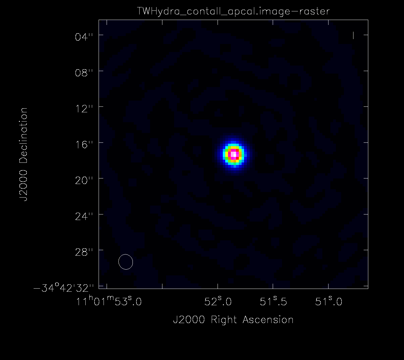
Compare the final image to the initial image and see if the image dynamic range has improve and phase- and amplitude-based errors have improved.

Finally, you should split out the results of your self-calibration for safe-keeping.

# in CASA
split(vis=contvis,
outputvis=contvis+'.selfcal', datacolumn='corrected')

If you are unhappy with the self-calibration, use the clearcal task and restore the original flags to return your ms to it’s original pre-self-cal state.

# in CASA
# uncomment the following to revert to pre self-cal ms
# flagmanager(vis=contvis, mode='restore',versionname='before_selfcal')
# clearcal(contvis)
# delmod(contvis,field=field,otf=True)

[xxx AAK there should be also a note on the best way to restart the self-cal process. This is somewhat complicated because it requires keeping track of the data, model, and corrected data columns as well as the flags. the easiest way to restart might be to put a split after the apply cal step in each round of self cal and do a copy of the ms before the first stepk but I need to think more about this.]

If you have line data, you will subtract the continuum and apply the self-calibration results to the line data on the next page, Spectral Line Imaging Template.

Return to the Main Page