Guide To Simulating ALMA Data

UNDER CONSTRUCTION

This guide is applicable to CASA version 4.1.

Introduction: Why Simulate ALMA Observations?

Observations made with radio interferometers can be tricky to interpret and analyze. Interferometers, by their nature, do not sample all spatial frequencies on the sky. Specifically, they are not sensitive to diffuse emission, and depending on a number of factors including the placement of the individual antennas, the length of the observation, and the location of the target source on the sky, an interferometric observation will be insensitive to some spatial structure in the sky brightness distribution. Observers therefore should use caution when analyzing and interpreting interferometric images.

Plots of "uv coverage" are often used to illustrate the range of spatial frequencies measured by a specific interferometric observation. The uv coverage plot can be thought of as a mask that is applied to the Fourier transform of the emission pattern on the sky. More densely sampled uv coverage leads to better images because the observation is more sensitive to a wider range of spatial frequencies on the sky.

To aid in interpreting their data, observers may find it helpful to simulate an interferometric observation using a variety of antenna configurations and different models of the sky brightness distribution. Simulations can also be a powerful tool to help new users understand both the power and the limitations of interferometric observations.

In some cases, those proposing to use ALMA may wish to simulate observations to bolster their ALMA proposal. For example, simulations can demonstrate the ability to resolve certain structures, and they can be used to justify the inclusion of compact or total power antennas.

Include Juergen's plot here.

There are several tools available on the web to help observers understand interferometric data and simulate observations. For example, those new to interferometry can get a basic understanding of how antenna placement affects uv coverage, the synthesized beam (i.e. the "resolution"), and the range of spatial sensitivities by exploring the Virtual Radio Interferometer. This is an interactive java application that allows one to simulate basic observations with MERLIN, ATCA, or WSRT, or ASKAP. The user can select from a few sample, idealized sky brightness patterns (e.g. a narrow gaussian) or use real sky brightness patterns, then fiddle interactively with the placement of antennas and the duration of the observation to see the effects of uv coverage on observations.

ALMA Simulation Tools

ALMA observers have two powerful simulation tools available: the CASA sim_observe/sim_analyze tasks, and the Observation Support Tool (OST). Both of these simulators are built on the CASA sm toolkit, and both are available from links on the ALMA Science Portal.

Note that significant differences may be seen between the noise predicted by the ALMA Sensitivity Calculator and the measured RMS in simulated images. These differences are primarily a result of the RMS measured in an image depending sensitively on the details of how the image is deconvolved. The ALMA sensitivity calculator is the primary tool used for time estimates during the technical assessment of ALMA proposals. Therefore, if using the results from the simulators in a Technical Justification of an observing proposal, users should discuss or reconcile any significant discrepancies between the RMS in the simulated image and that determined by the sensitivity calculator.

The OST

The OST is a web-based interface hosted by the EU ARC at the University of Manchester. Users who do not have experience with CASA, and who do not need full control of the simulation and imaging process will usually find the OST a good choice for generating simulated images. The GUI works in a straightforward top-down approach. Full documentation for the OST is available here.

The OST determines atmospheric opacity in a slightly different way than the CASA sim tasks, and so it may return slightly results from the CASA sin tasks. The differences are most noticeable for simulations in Bands 9 and 10.

CASA simulation tools

Simulating ALMA observations in CASA proceeds in the following steps:

1. Make a model image. This is a representation of the sky brightness distribution that you would like to simulate observing. There are several paths to making a model image, discussed below.
2. Generate uv data with the simobserve task.
3. Image the simulated observation with the simanalyze task.

The simobserve task generates the visibilities that would be measured by observing the specified input model of sky brightness. The user needs to specify a telescope to use for the observation. CASA includes a set of configuration files for ALMA, the VLA, CARMA, the SMA, ATCA, and the Plateau de Bure interferometers. The specific configuration files shipped with a CASA installation are available here. The simobserve task can add thermal noise to the visibilities. The simobserve task uses the aatm atmospheric model (based on Juan Pardo's ATM library) to simulate real observing conditions and introduce atmospheric "corruption", i.e. noise and phase delay.

Next, the simanalyze task is used to produce a cleaned image based on the generated visibilities. It can compare the simulated image with your input (convolved with the output clean beam) and then calculate a "fidelity image" that indicates how well the simulated output matches the convolved input image.

Generating a Model Image

A "model image" is a FITS file that contains a representation of the sky brightness distribution, and it represents the object to be "observed" in the simulation. The FITS file must contain a realistic set of spatial axes, and a realistic flux density. There are several ways to generate a model image.

1. An existing FITS image.

The simplest option is to begin with an existing FITS image of a millimeter or submillimeter observation. The FITS image can be either a single plane (i.e. one observed frequency channel) or a cube. A common simulation exercise is to begin with a FITS file representing an observation of a target, then scale the spatial axes and the flux to shift the data to what would be observed for a similar target at a different distance.

The simobserve task can scale the image from the FITS file directly. The task uses parameters inbright, indirection, incell, incenter, and inwidth to set the peak flux density, coordinates on the sky, pixel size, frequency of the center channel, and channel width, respectively.

1. A component list.

It may be useful to simulate observations of an idealized model image consisting, for example, of point sources and Gaussians. The CASA component list tool (cl) allows the user to create a FITS file by specifying a set of point sources, Gaussians, disks, and limb-darkened disks. Each of these is a "component" in the FITS image. This CASA guide provides an example of creating a FITS file from a component list.

1. A GIF or JPG image

A user may wish to convert a GIF or JPG image to a FITS file for simulation in CASA. The image should be converted to a 16-bit FITS image for use with the CASA sim tools. See this page for an example of using gimp to convert a JPG image to a FITS file. Alternatively, you could use ImageMagik, like so:

convert myfile.jpg myfile.fits

Then proceed to trim and convert the file in CASA like so:

importfits(fitsimage='myfile.fits',imagename='testimage',overwrite=T)
default 'immath'
imagename = 'testimage'
expr = 'IM0'
box = '0,0,299,299'
outfile = 'testimage2'
immath()
exportfits(imagename ='testimage2',fitsimage ='myfile_16bit.fits',bitpix=16,overwrite=T)

Generating visibilities with simobserve

The task simobserve takes several steps to generate observed visibilities.

• Modify Model. If desired, you can modify the header parameters in your data model to mimic different observing targets. For example, if you start with a model of M100 you might wish to scale the axes to simulate an observation of an M100-like galaxy that is 4X more distant. The settable parameters include:
  • inbright: Scaling the model flux densities by setting the peak flux density of the brightest pixel, e.g. "1.2Jy/pixel"
  • indirection: Set the center target coordinates, e.g. "J2000 19h00m00 -40d00m00"
  • incell: Set the angular size of each pixel, e.g. "0.1arcsec"
  • incenter: Set the observed sky frequency. If the model is a spectral cube, this parameter applies to the center channel.
  • inwidth: Set the channel width, e.g. "10MHz"
• Set Pointings. If the angular size of your model image is comparable or larger than the 12-m primary beam, you can simulate observing the target as a mosaic. In this step, the individual pointings are determined and saved in a text file. You can also generate such a text file yourself.
• Generate visibilities. The visibilities are determined based on the telescope and configuration specified, and the length in time of the observation.
• Add noise. Finally, noise is added to the visibilities.

Transforming to images with simanalyze

Both simobserve and simanalyze can be broken down into a number of steps. The major steps are:

1. simobserve
   1. Modify Model - If desired, you can scale the spatial coordinates, spectral axis, and brightness of the sky model image to simulate a specific type of observation. (For example, if you start with a model of M100 you might wish to scale the axes to simulate an observation of an M100-like galaxy that is 4X more distant.)
   2. Set Pointings - If your simulation contains multiple pointings in a mosaic, calculate the positions of individual pointings. These are saved in a text file. (You could also make such a text file yourself.)
   3. Predict - Calculate the visibilities. You will specify a telescope, antenna configuration, and date for the simulated observation.
   4. Corrupt - Next, "corrupt" the data, for example by introducing with thermal noise or phase noise.
2. simanalyze
   1. Image - Image the visibility data with CASA's clean task.
   2. Analyze - Calculate and display the difference between output and input, and the fidelity image.

The Simulation Guide for New Users tutorial introduces and explains the individual steps in detail. It is possible to run the steps independently and optionally, as long as you follow the simobserve and simanalyze conventions about filenames.

Taskname History

The simulation tasks have been under significant revision and development.

• In CASA 3.3 simobserve and simanalyze were named sim_observe and sim_analyze, respectively.
• In CASA 3.4 and earlier, the functionality of both tasks was contained in task simdata, which is now obsolete.
• In CASA 4.1, a new experimental task simalma has been introduced, which simplifies simulation of 12m interferometric + 7m interferometric + total power ALMA observations. Please report any issue with simalma, and check back here for an upcoming simalma casaguide.

Values from simobserve or the OST should not be used to calculate exposure times for ALMA Science Goals. Only values from the ALMA sensitivity calculator should be used for this purpose, as it is the ALMA sensitivity calculator that will be used in the technical assessment of ALMA proposals. However, the results of simulations may be helpful to support a request for more observing time than is required by the sensitivity calculator, in order to obtain better uv-plane coverage.

Tutorials

Simulation Guide for New Users (CASA 4.1)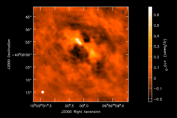
A fully annotated tutorial that uses a Spitzer SAGE 8 micron continuum image of 30 Doradus and scales it to greater distance. A good place for new users to start.
Protoplanetary Disk Simulation (CASA 4.1)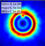
A sky model with a lightly annotated script that simulates a protoplanetary disk. Uses a theoretical model of dust continuum from Sebastian Wolff, scaled to the distance of a nearby star. This is another fairly generic simulation - if you're short on time, you probably don't need to go through this one and the New Users guide, but it can be useful to go through multiple examples.
Simulation Guide Component Lists (CASA 4.1)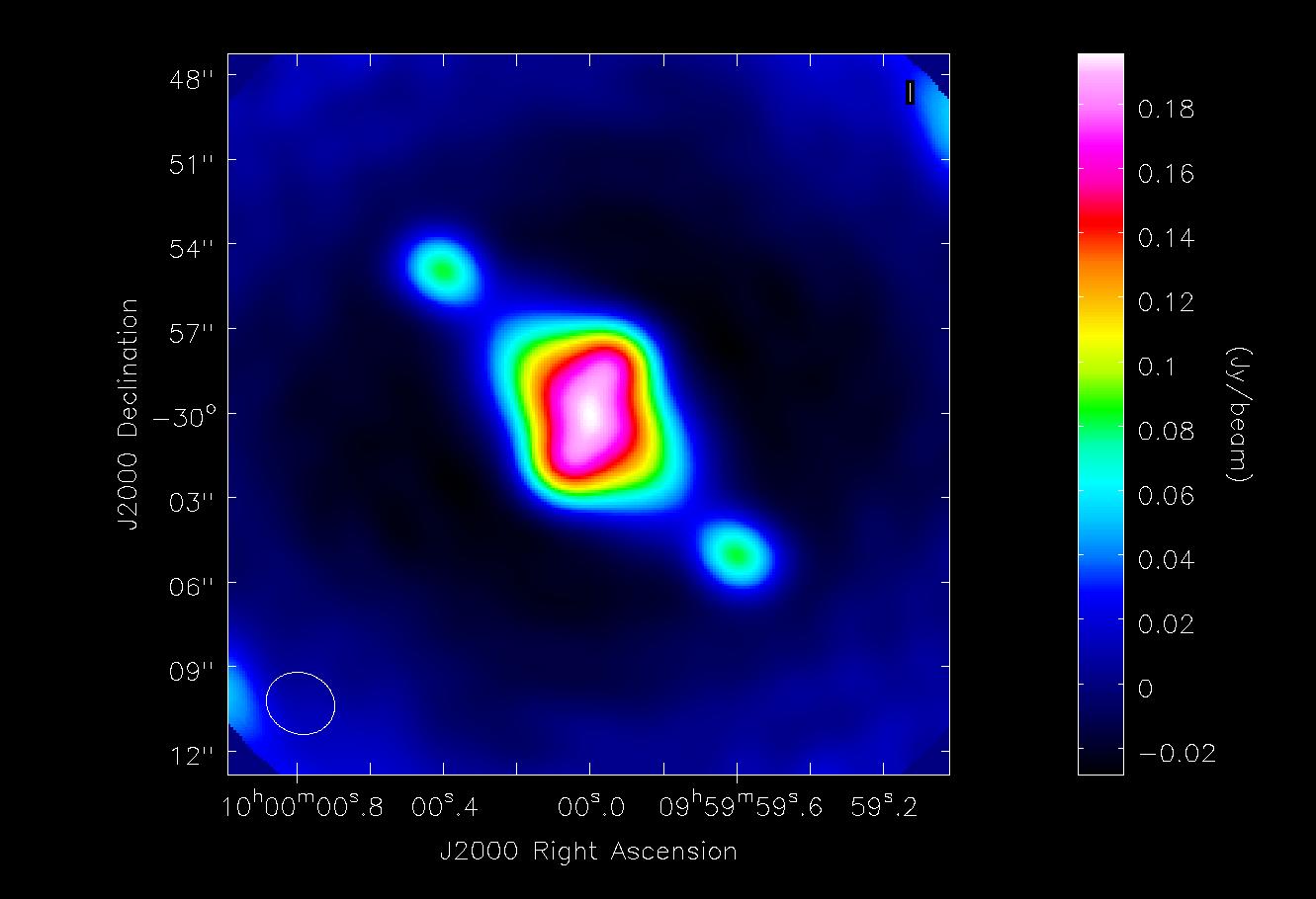
Tutorial for simulating data based on multiple sources (using both a FITS image and a component list). If you are interested in simulating from a list of simple sources (point, Gaussian, disk), rather than or in addition to a sky model image, then read the considerations here.
Einstein-Face (CASA 4.1)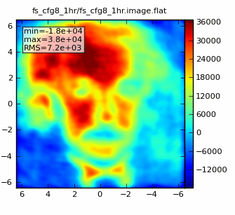
A sky model and lightly annotated script that simulates the face of Einstein as seen by ALMA. This simulation is particularly useful for those who wish to better understand spatial filtering by an interferometer, but doesn't demonstrate new capabilities of the simulation tasks beyond those described above.
ACA Simulation (CASA 4.1)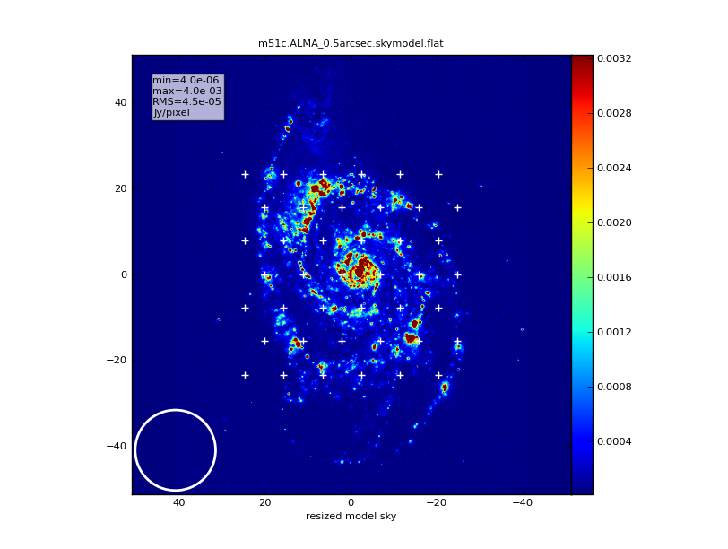
A tutorial for simulating ALMA observations that use multiple configurations or use the 12-meter array in combination with the ALMA Compact Array. This tutorial demonstrates combining data from each ALMA component "by hand". This guide is of particular interest to those wishing to explore using the 12-m array in combination with the ACA, and those interested in combining data from multiple 12-m array configurations.
simalma
This tutorial demonstrates how to use simalma, a task that simplifies simulations that include the main 12-m array plus the ACA. Like the previous guide, this one is of particular interest to those wishing to explore multi-component ALMA observations.

Example Input Images

Several examples of input model images are showcased here: Sim Inputs. These may be useful for running your own simulation tests, beyond what are presented in the above tutorials.

Advanced CASA Simulation

Under the Hood: The sm Tool

simobserve calls methods in the sm (simulation) tool. For advanced CASA users, the sm tool has methods that can add to simulated data: phase delay variations, gain fluctuations and drift, cross-polarization, and (coming soon) bandpass and pointing errors. sm also has more flexibility than simobserve in adding thermal noise. The tutorials linked from this page describe the simulation of data using the task interface only. To learn more about the sm tool, see the CASA Toolkit Reference Manual.

The sm tool can be used to corrupt your measurement set with thermal noise, phase noise, cross-polarization, etc., in a more advanced way than is done in simobserve. To learn advanced techniques for corrupting a simulated measurement set, see Corrupt.

Ephemeris and Geodesy

Generic ephemeris and geodesy calculations can be done using CASA Python module simutil.py.

Warning: CLEAN Bias

As is the case for real images, cleaning images produced by simobserve can lead to a spurious decrease in object fluxes and noise on the image (an effect known as "clean bias"). This is particularly true for observations with poor coverage of the uv-plane, i.e. using telescopes with small numbers of antennas, such as the ALMA Early Science configurations, and/or in short "snapshot" observations. Users should always clean images with care, using a small number of iterations and/or a conservative (3-5sigma) threshold and boxing bright sources.

User Feedback

We welcome input on developing the CASA simulator. Contact "rindebet at nrao.edu" if you would like to volunteer your input.