Simulating Observations in CASA 4.0

UNDER DEVELOPMENT

• This guide is applicable to CASA version 4.0. For older versions of CASA please see Simulating Observations in CASA 3.4.

Introduction

The task simobserve can be used to simulate an observation in CASA. simobserve turns a model of the sky (2 to 4 dimensions including frequency and polarization) into the visibilities that would be measured with ALMA, (E)VLA, CARMA, SMA, ATCA, PdB, et cetera. simobserve can also add thermal noise (from receiver, atmosphere, and ground) to the visibilities. simobserve uses the aatm atmospheric model, a thin wrapper of Juan Pardo's ATM library, to accurately calculate all atmospheric corruption terms (noise, phase delay) accurately as a function of frequency and site characteristics.

After creating the visibilities, task simanalyze will produce a cleaned image of the model visibilities, compare that image with your input convolved with the synthesized beam, and calculate a fidelity image.

Taskname History The simulation tasks have been under significant revision and development.

• In CASA 3.3 simobserve and simanalyze were named sim_observe and sim_analyze, respectively.
• In CASA 3.4 and earlier, the functionality of both tasks was contained in task simdata, which is now removed.
• In CASA 4.0, a new experimental task simalma has been introduced, which simplifies simulation of 12m interferometric + 7m interferometric + total power ALMA observations. Please report any issue with simalma, and check back here for an upcoming simalma casaguide.

Simulating ALMA Observations

Although simobserve can simulate data for many instruments, this guide (and the tutorials linked below) focuses in particular on simulating ALMA observations. ALMA is still under construction. We will update CASA's simulation tasks and tools as ALMA commissioning proceeds. During this period, we expect the noise properties of the telescope to be increasingly better characterized, and its configurations to be refined.

Users should be aware of the Observation Support Tool (OST) [1]. This is a web-based interface to an ALMA simulator hosted by the University of Manchester, UK. Like the simobserve, it is based on the CASA sm toolkit, but uses different wrapper scripts, and, in particular, has a different treatment of atmospheric effects. Comparisons to the ALMA sensitivity calculator made in March 2011 suggest that both simobserve and the OST give similar noises for observations in bands 3 to 8. However, the OST diverges in bands 9 and 10.

Since the ALMA sensitivity calculator will be used for the technical assessment of ALMA proposals, only values from it, not simobserve or the OST, should be used to estimate exposure times for ALMA Science Goals.

Tutorials

Simulation Guide for New Users (CASA 4.0)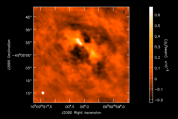
A fully annotated tutorial that uses a Spitzer SAGE 8 micron continuum image of 30 Doradus and scales it to greater distance.
Simulation Guide Component Lists (CASA 4.0)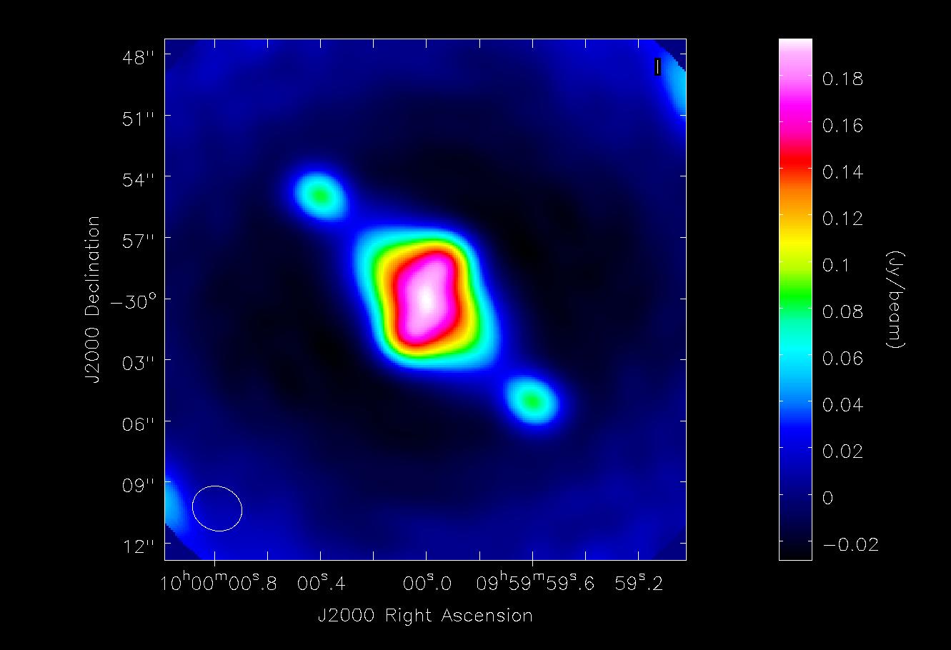
Tutorial for simulating data based on multiple sources (using both a FITS image and a component list).
Protoplanetary Disk Simulation (CASA 4.0)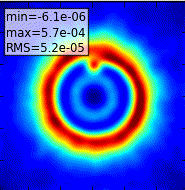
A sky model with a lightly annotated script that simulates a protoplanetary disk. Uses a theoretical model of dust continuum from Sebastian Wolff, scaled to the distance of a nearby star.
Einstein-Face (CASA 4.0)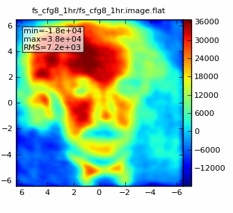
A sky model and lightly annotated script that simulates the face of Einstein as seen by ALMA. Uses a non-science image to demonstrate the effects of spatial filtering by ALMA.
ACA Simulation (CASA 4.0)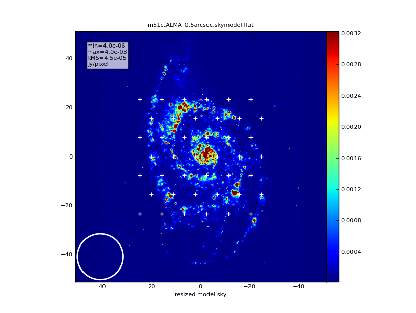
A tutorial for simulating ALMA observations that use multiple configurations or use the 12-meter array in combination with the ALMA Compact Array.

Example Input and Output

Several examples of input model images are showcased here: Sim Inputs.

Several examples of simanalyze output images are showcased here: Sim Outputs.

Advanced CASA Simulation

Step-by-Step Simulations

simobserve and simanalyze can be broken down into a series of steps, each of which is modular. As long as you follow a few conventions about filenames, you can run each bit independently and optionally. For example, using simobserve, you can modify the sky model, then predict ACA visibilities, then run again and predict ATCA 12m visibilities. With simanalyze you can image and analyze both the ACA and ATCA measurement sets together. You can run interactive clean yourself, and, minding your filenames, you can run simanalyze just to calculate a difference image and analyze the results.

The major steps involved in simulating data with CASA are:

1. simobserve
   1. Modify Model - relabel (scale) the spectral and spatial coordinates and brightness of the sky model image.
   2. Set Pointings - calculate a mosaic of pointings and save in a text file. You could also make the text file yourself.
   3. Predict - Calculate visibilities for a specified array on a specified day.
   4. Corrupt - Corrupt the measurement set with thermal noise, phase noise, cross-polarization, etc.
2. simanalyze
   1. Image - Image the visibility data with clean.
   2. Analyze - Calculate and display the difference between output and input, and fidelity image.

Under the Hood: The sm Tool

simobserve calls methods in the sm tool. For advanced users, sm has methods that can add phase delay variations, gain fluctuations and drift, cross-polarization, and (coming soon) bandpass and pointing errors to simulated data. sm also has more flexibility in adding thermal noise than simobserve. The tutorials linked from this page describe the simulation of data using the task interface only. To learn more about sm, see the CASA Toolkit Reference Manual.

Ephemeris and Geodesy

Generic ephemeris and geodesy calculations can be done using CASA Python module simutil.py.

Warning: CLEAN Bias

As is the case for real images, cleaning images produced by simobserve can lead to a spurious decrease in object fluxes and noise on the image ("clean bias"). This is particularly true for observations with poor coverage of the uv-plane, i.e. using telescopes with small numbers of antennas, such as the ALMA Early Science configurations, and/or in short "snapshot" observations. Users should always clean images with care, using a small number of iterations and/or a conservative (3-5sigma) threshold and boxing bright sources.

User Feedback

We welcome input on developing the CASA simulator. Contact "rindebet at nrao.edu" if you would like to volunteer your input.