NGC 5921: red-shifted HI emission 5.7.2: Difference between revisions
| Line 320: | Line 320: | ||
refant = '15' | refant = '15' | ||
saveinputs('bandpass',prefix+'.bandpass.saved') | saveinputs('bandpass',prefix+'.bandpass.saved') | ||
bandpass() | bandpass() | ||
</source> | </source> | ||
Revision as of 14:15, 14 December 2009
Overview
The technique used to calibrate and image continuum datasets generally applies to spectral line observations, except that an additional calibration step is required. Bandpass calibration flattens the spectral response of the observations, ensuring that spectral channel images are properly calibrated in amplitude and phase.
The following tutorial derives from an annotated script provided in the CASA Cookbook. The script is largely reproduced and additionally annotated with figures and illustrations. It is assumed that this tutorial will be used interactively, and so interactive pauses in the original script have been removed.
The data are included with the CASA installation.
Setting up the CASA Environment
Start up CASA in the directory you want to use.
# in bash
mkdir NGC5921
cd NGC5921
casapy
Now, in CASA, set up paths and global variables to facilitate the data reduction. These operations can be performed on-the-fly if you are reducing data interactively, but it's better to have them prepared from the start in the scripting environment.
import os
scriptmode = True

prefix = 'ngc5921.demo' # The prefix to use for all output files
# Set up some useful variables (these will be altered later on)
msfile = prefix + '.ms'
btable = prefix + '.bcal'
gtable = prefix + '.gcal'
ftable = prefix + '.fluxscale'
splitms = prefix + '.src.split.ms'
imname = prefix + '.cleanimg'
We'll use a python os command to get the appropriate CASA path for your installation. The use of os.environ.get is explained in the Appendix.
pathname=os.environ.get('CASAPATH').split()[0]
fitsdata=pathname+'/data/demo/NGC5921.fits'
Scripts are of course modified and repeated to the satisfaction of observer. To help clean up the bookkeeping and further avoid issues of write privileges, remove prior versions of the measurement set and calibration tables.
Tip: The first command in the following code block removes the measurement set. Depending on the size of the source data, refilling a measurement set can be time-consuming, and so you may want to consider editing a separate script that preserves the measurement set but skips the importuvfits command given below. This NGC5921 dataset, however, is not large and refilling goes quickly.
rmtables(msfile)
rmtables(btable)
rmtables(gtable)
rmtables(ftable)
rmtables(ftable)
rmtables(splitms+'*')
rmtables(imname+'.*')
rmtables(prefix+'.moments*')

# Final clean up of auxiliary files
os.system('rm -rf '+prefix+'*')
Import the Data
The next step is to import the multisource UVFITS data to a CASA measurement set via the importuvfits filler.
# Safest to start from task defaults
default('importuvfits')
# Set up the MS filename and save as new global variable
msfile = prefix + '.ms'
# Use task importuvfits
fitsfile = fitsdata
vis = msfile
saveinputs('importuvfits',prefix+'.importuvfits.saved')
importuvfits()
Saveinputs saves the parameters of a given command to specified text file, handy to debug a script and see what actually was run. The parameters of importuvfits are saved to the file "ngc5921.demo.importuvfits.saved". A listing of this file follows. Notice that it is executable with execfile in CASA (remove the # commenting symbol before importuvfits to have the execfile run the command).
CASA <71>: os.system('cat ngc5921.demo.importuvfits.saved')
taskname           = "importuvfits"
fitsfile           =  "/usr/lib64/casapy/30.0.9709test-001/data/demo/NGC5921.fits"
vis                =  "ngc5921.demo.ms"
antnamescheme      =  "old"
#importuvfits(fitsfile="/usr/lib64/casapy/30.0.9709test-001/data/demo/NGC5921.fits",vis="ngc5921.demo.ms",antnamescheme="old")
A Summary of the Data
We'll need to have a look at the observing tables to learn the calibrator and source names. The relevant command is listobs.
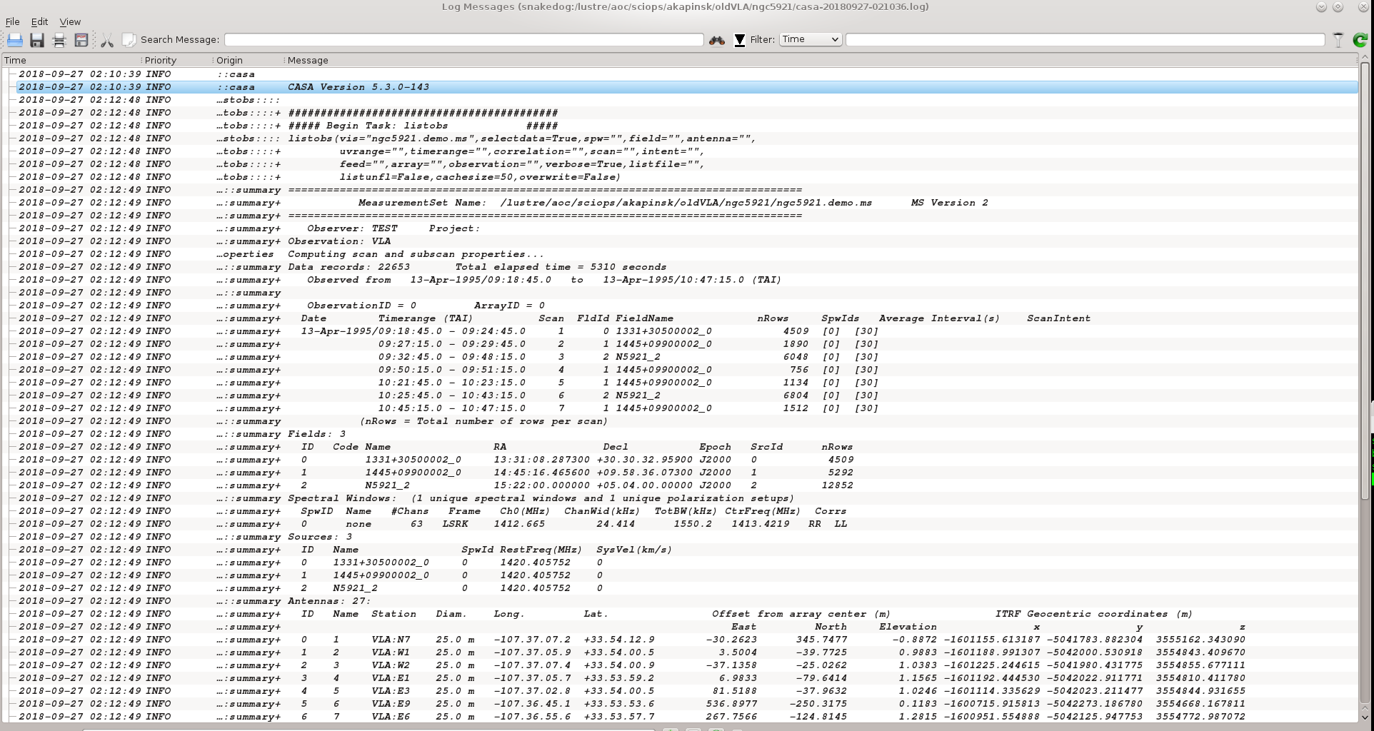
listobs(vis='ngc5921.demo.ms', verbose=True)
The output goes to the logger window; see the screenshot at right.
Tip: You can control the text size of the logger window using <ctrl>-A (smaller font) and <ctrl>-L (larger font).
A more complete listing of the listobs output follows.
INFO listobs	##### Begin Task: listobs            #####
INFO  	listobs::::casa
================================================================================
           MeasurementSet Name:  /DATA/ASHLESHA_2/NGC5921/ngc5921.demo.ms      MS Version 2
================================================================================
   Observer: TEST     Project:
Observation: VLA
Data records: 22653       Total integration time = 5280 seconds
   Observed from   13-Apr-1995/09:19:00.0   to   13-Apr-1995/10:47:00.0 (TAI)
2009-12-03 16:15:38 INFO  	listobs::ms::summary
   ObservationID = 0         ArrayID = 0
  Date        Timerange (TAI)          Scan  FldId FieldName    nVis   Int(s)   SpwIds
  13-Apr-1995/09:19:00.0 - 09:24:30.0     1      0 1331+305000* 4509   30       [0]
              09:27:30.0 - 09:29:30.0     2      1 1445+099000* 1890   30       [0]
              09:33:00.0 - 09:48:00.0     3      2 N5921_2      6048   30       [0]
              09:50:30.0 - 09:51:00.0     4      1 1445+099000* 756    30       [0]
              10:22:00.0 - 10:23:00.0     5      1 1445+099000* 1134   30       [0]
              10:26:00.0 - 10:43:00.0     6      2 N5921_2      6804   30       [0]
              10:45:30.0 - 10:47:00.0     7      1 1445+099000* 1512   30       [0]
           (nVis = Total number of time/baseline visibilities per scan)
Fields: 3
  ID   Code Name         RA            Decl           Epoch   SrcId nVis
  0    C    1331+305000* 13:31:08.2873 +30.30.32.9590 J2000   0     4509
  1    A    1445+099000* 14:45:16.4656 +09.58.36.0730 J2000   1     5292
  2         N5921_2      15:22:00.0000 +05.04.00.0000 J2000   2     12852
   (nVis = Total number of time/baseline visibilities per field)
Spectral Windows:  (1 unique spectral windows and 1 unique polarization setups)
  SpwID  #Chans Frame Ch1(MHz)    ChanWid(kHz)TotBW(kHz)  Ref(MHz)    Corrs
  0          63 LSRK  1412.66507  24.4140625  1550.19688  1413.42801  RR  LL
Sources: 3
  ID   Name         SpwId RestFreq(MHz)  SysVel(km/s)
  0    1331+305000* 0     1420.405752    0
  1    1445+099000* 0     1420.405752    0
  2    N5921_2      0     1420.405752    0
Antennas: 27:
  ID   Name  Station   Diam.    Long.         Lat.
  0    1     VLA:N7    25.0 m   -107.37.07.2  +33.54.12.9
  1    2     VLA:W1    25.0 m   -107.37.05.9  +33.54.00.5
  2    3     VLA:W2    25.0 m   -107.37.07.4  +33.54.00.9
  3    4     VLA:E1    25.0 m   -107.37.05.7  +33.53.59.2
  4    5     VLA:E3    25.0 m   -107.37.02.8  +33.54.00.5
  5    6     VLA:E9    25.0 m   -107.36.45.1  +33.53.53.6
  6    7     VLA:E6    25.0 m   -107.36.55.6  +33.53.57.7
  7    8     VLA:W8    25.0 m   -107.37.21.6  +33.53.53.0
  8    9     VLA:N5    25.0 m   -107.37.06.7  +33.54.08.0
  9    10    VLA:W3    25.0 m   -107.37.08.9  +33.54.00.1
  10   11    VLA:N4    25.0 m   -107.37.06.5  +33.54.06.1
  11   12    VLA:W5    25.0 m   -107.37.13.0  +33.53.57.8
  12   13    VLA:N3    25.0 m   -107.37.06.3  +33.54.04.8
  13   14    VLA:N1    25.0 m   -107.37.06.0  +33.54.01.8
  14   15    VLA:N2    25.0 m   -107.37.06.2  +33.54.03.5
  15   16    VLA:E7    25.0 m   -107.36.52.4  +33.53.56.5
  16   17    VLA:E8    25.0 m   -107.36.48.9  +33.53.55.1
  17   18    VLA:W4    25.0 m   -107.37.10.8  +33.53.59.1
  18   19    VLA:E5    25.0 m   -107.36.58.4  +33.53.58.8
  19   20    VLA:W9    25.0 m   -107.37.25.1  +33.53.51.0
  20   21    VLA:W6    25.0 m   -107.37.15.6  +33.53.56.4
  21   22    VLA:E4    25.0 m   -107.37.00.8  +33.53.59.7
  23   24    VLA:E2    25.0 m   -107.37.04.4  +33.54.01.1
  24   25    VLA:N6    25.0 m   -107.37.06.9  +33.54.10.3
  25   26    VLA:N9    25.0 m   -107.37.07.8  +33.54.19.0
  26   27    VLA:N8    25.0 m   -107.37.07.5  +33.54.15.8
  27   28    VLA:W7    25.0 m   -107.37.18.4  +33.53.54.8
2009-12-03 16:15:38 INFO  	listobs::::casa
##### End Task: listobs              #####
##########################################
Key Information from Listobs
Certainly the output of listobs is dense with information, but there are some particularly vital data that we'll need for the calibration.
- The calibrators are 1331+305* (3C286, the flux and bandpass calibrator) and 1445+099* (the phase calibrator). We can use wild-cards 1331* and 1445* since they uniquely identify the sources.
- The calibrator field indices are field='0' (1331+305) and field='1' (1445+099).
- The name of the source in the observations list is N5921_2, or field = '2'.
- The data were taken in a single IF (a single spectral window, SpwID = 0), divided into 63 channels.
- Only RR and LL correlations are present; cross-pols are absent.
Flagging
Flag the autocorrelations
We don't need the autocorrelation data, and flagautocorr gets rid of them. You shouldn't have to specify the measurement set, because the variable vis is already set, but it never hurts to be cautious.
flagautocorr(vis="ngc5921.demo.ms")
Interactive Flagging
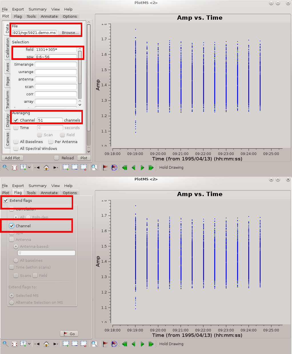
Casaplotms is a good tool for flagging spectral line data. Check out the tutorial that describes editing VLA continuum data. Spectral line data of course require some consideration of channels and channel averaging.
Casaplotms currently runs outside the CASA python shell, but we can use os.system to start it from within CASA. In the following code snippet, the command is commented out to provide a non-interactive this tutorial. Uncomment to include interactive data editing as part of the script.
# os.system("casaplotms")
The figure at right highlights the settings needed for effective editing of a spectral line data set. The key settings are as follows.
- Specify the measurement set in File Location; the Browse button allows you to hunt down the measurement set.
- It's better to edit one source at a time. In the illustrated example, the flux / bandpass calibrator 1331+305* is displayed.
- Average the channels. First, specify the central channels to remove band edge effects. Channels 6~56 in the first spectral window (IF) are appropriate (see #Inspect the Bandpass Response Curve, below). In the Channel Averaging box, enter 51 channels to average over all channels in the given range.
- Ideally you want the channels to have the same (u, v) coverage (projected baseline spacings as viewed from the source); otherwise, the beam (point spread function) will be different for each channel. Therefore, if you flag data from a given channel it's usually a good idea to flag those data from all channels. Under the Flagging tab, specify Extend flags to Channel.
With these settings, interactive flagging proceeds as for continuum data. When you're satisfied with the edits, File → Quit to return to the CASA prompt.
Calibration
Calibration of spectral line data broadly follows the approach for continuum data, except that the amplitude and phase corrections are a function of frequency and so must be corrected by bandpass calibration. The basic calibration steps follow.
- Set the flux scale of the primary calibrator, here, 1331+305 = 3C 286.
- Determine bandpass corrections based on the primary calibrator. In the script that follows, the bandpass calibration is stored in ngc5921.demo.bcal, which is itself referenced by the python variable btable.
- Inspect the bandpass correction to determine viable channels for averaging and imaging. We want to toss out end channels where the response is poor.
- Determine the gain calibrations on the bandpass-corrected and channel-averaged data. In this step, we effectively turn the spectral line data into a single-channel continuum data set and calibrate accordingly. The calibration is stored in ngc5921.demo.gcal, which is itself referenced by the python variable gtable.
- Inspect the gain calibration solutions to look for any aberrant solutions that hint at bad calibrator data.
- Apply the calibration solutions to the source (N5921_2). This action literally adds a new column of data to the measurement set. This new column contains the data with the gain calibration and bandpass calibration applied, but it does not overwrite the raw data in case the calibration needs revision.
Setting the Flux Scale
Setjy generates a point source model for the primary calibrator, 1331+305 = 3C286. These data are of low angular resolution, and so the point source model is adequate for our purposes. For observations with higher angular resolution (longer baseline configurations), you can specify a model of the calibrator using the modimage parameter (see the tutorial Calibrating a VLA 5 GHz continuum survey#Set the Flux Scale for an example of how to use modimage).
Setjy also looks up the radio SED for common flux calibrators and automatically assigns the total flux density.
default('setjy')
vis = msfile
#
# 1331+305 = 3C286 is our primary calibrator
# Use the wildcard on the end of the source name
# since the field names in the MS have inherited the
# AIPS qualifiers
field = '1331+305*'
# This is 1.4GHz D-config and 1331+305 is sufficiently unresolved
# that we dont need a model image.  For higher frequencies
# (particularly in A and B config) you would want to use one.
modimage = ''
# Setjy knows about this source so we dont need anything more
saveinputs('setjy',prefix+'.setjy.saved')
setjy()
A summary of the operation is sent to the logger window. Here's a listing of the output.
2009-12-07 15:44:22 INFO  	setjy::::casa
2009-12-07 15:44:22 INFO setjy	##########################################
2009-12-07 15:44:22 INFO setjy	##### Begin Task: setjy              #####
2009-12-07 15:44:22 INFO  	setjy::::casa
2009-12-07 15:44:22 INFO setjy	Adding MODEL_DATA, CORRECTED_DATA and IMAGING_WEIGHT columns
2009-12-07 15:44:23 INFO setjy	Initializing MODEL_DATA (to unity) and CORRECTED_DATA (to DATA)
2009-12-07 15:44:25 INFO setjy	Initialized 22653 rows.
2009-12-07 15:44:25 INFO setjy	Initializing natural weights
2009-12-07 15:44:25 INFO setjy	1331+30500002_0  spwid=  0  [I=14.76, Q=0, U=0, V=0] Jy, (Perley-Taylor 99)
2009-12-07 15:44:25 INFO setjy	Selecting data
2009-12-07 15:44:25 INFO setjy	Selected 4509 out of 22653 visibilities.
2009-12-07 15:44:25 INFO setjy	Fourier transforming: replacing MODEL_DATA column
2009-12-07 15:44:25 INFO setjy	Processing after subtracting componentlist /DATA/ASHLESHA_2/NGC5921/ngc5921.demo.ms.1331+30500002_0.spw0.tempcl
2009-12-07 15:44:25 INFO setjy	Performing interferometric gridding with convolution function SF
2009-12-07 15:44:25 INFO  	setjy::::casa
2009-12-07 15:44:25 INFO setjy	##### End Task: setjy                #####
2009-12-07 15:44:25 INFO setjy	##########################################
Bandpass Calibration
The flux calibrator 1331+305 = 3C 286 now has a point-source model assigned to it. Since the point-source model doesn't change over this narrow range of frequencies, we can use the model to determine amplitude and phase (gain) corrections for each channel independently. The result is the bandpass calibration.
As for any antenna-based calibration scheme, we have to pick an antenna to act as the reference point for the calibration. Any antenna will do, but it's better to pick one near the center of the array. For the remainder of the calibration, we will use refant = '15'.
default('bandpass')
# We can first do the bandpass on the single 5min scan on 1331+305
# At 1.4GHz phase stablility should be sufficient to do this without
# a first (rough) gain calibration.  This will give us the relative
# antenna gain as a function of frequency.
vis = msfile
# set the name for the output bandpass caltable
btable = prefix + '.bcal'
caltable = btable
# No gain tables yet
gaintable = ''
gainfield = ''
interp = ''
# Use flux calibrator 1331+305 = 3C286 (FIELD_ID 0) as bandpass calibrator
field = '0'
# all channels
spw = ''
# No other selection
selectdata = False
# In this band we do not need a-priori corrections for
# antenna gain-elevation curve or atmospheric opacity
# (at 8GHz and above you would want these)
gaincurve = False
opacity = 0.0
# Choose bandpass solution type
# Pick standard time-binned B (rather than BPOLY)
bandtype = 'B'
# set solution interval arbitrarily long (get single bpass)
solint = 'inf'
combine = 'scan'
# reference antenna Name 15 (15=VLA:N2) (Id 14)
refant = '15'
saveinputs('bandpass',prefix+'.bandpass.saved')
bandpass()
Inspect the Bandpass Response Curve
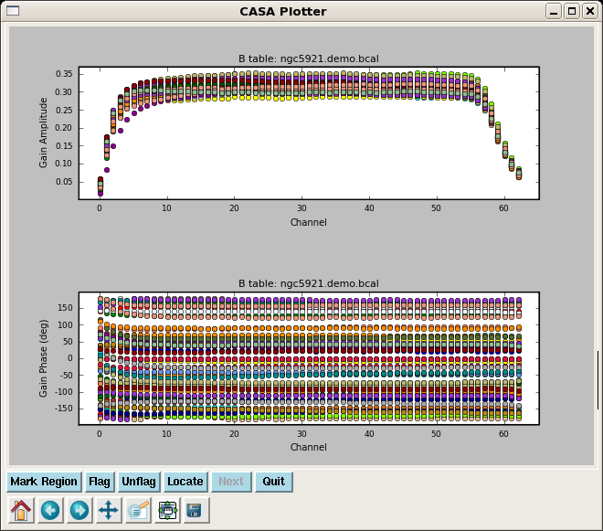
In the gain calibration to follow, we will effectively convert the spectral line data into a continuum data set. Before proceeding, we need to inspect the bandpass calibration to make sure that it contains no bad values and also to inspect which channels to average to produce the continuum data. Plotcal is the standard tool for plotting calibration solutions. The following script produces the figure at right.
By inspection, the amplitude response curve is flat over channels 6~56; that channel range will be used to generate the continuum data for gain calibration.
Notice that plotcal is run twice: once to display gain amplitudes as a function of channel (frequency), and again to plot gain phases as a function of channel.
If the scriptmode is set to False, the plot is saved to ngc5921.demo.plotcal.png.
#
#=====================================================================
#
# Use plotcal to examine the bandpass solutions
#
print '--Plotcal (bandpass)--'
default('plotcal')
caltable = btable
field = '0'
# Set up 2x1 panels - upper panel amp vs. channel
subplot = 211
yaxis = 'amp'
# No output file yet (wait to plot next panel)
saveinputs('plotcal',prefix+'.plotcal.b.amp.saved')
if scriptmode:
    showgui = True
else:
    showgui = False
plotcal()
#
# Set up 2x1 panels - lower panel phase vs. channel
subplot = 212
yaxis = 'phase'
saveinputs('plotcal',prefix+'.plotcal.b.phase.saved')
#
# Note the rolloff in the start and end channels.  Looks like
# channels 6-56 (out of 0-62) are the best
# Pause script if you are running in scriptmode
if scriptmode:
    # If you want to do this interactively and iterate over antenna, set
    # iteration = 'antenna'
    showgui = True
    plotcal()
    user_check=raw_input('Return to continue script\n')
else:
    # No GUI for this script
    showgui = False
    # Now send final plot to file in PNG format (via .png suffix)
    figfile = caltable + '.plotcal.png'
    plotcal()
Gain Calibration
From inspection of the bandpass response curve, we can average channels 6~56 to produce continuum data for the calibrators. For VLA data, this averaging is specified through the spw (spectral window) parameter, which takes the form IF:Channel-range, as follows.
spw = '0:6~56'
That is, there is only one spectral window (IF), spw = 0, and we want to average channels 6~56 within that spectral window.
Gain calibrations are otherwise determined as for continuum data.
- gaincal() is run only on the calibrators, 1331+305 (flux calibrator) and 1445+099 (phase calibrator).
- The default model for gain calibrations is a 1 Jy point-source. The flux scale is overridden by setjy, which has been performed for the flux calibrator. We need to transfer that flux scale to the phase calibrator using fluxscale().
- Note that fluxscale() determines the flux density of the phase calibrator and accordingly adjusts its model and calibration solutions. A report of the results are sent to the logger window.
#=====================================================================
#
# Gain calibration
#
print '--Gaincal--'
default('gaincal')
# Armed with the bandpass, we now solve for the
# time-dependent antenna gains
vis = msfile
# set the name for the output gain caltable
gtable = prefix + '.gcal'
caltable = gtable
# Use our previously determined bandpass
# Note this will automatically be applied to all sources
# not just the one used to determine the bandpass
gaintable = btable
gainfield = ''
# Use nearest (there is only one bandpass entry)
interp = 'nearest'
# Gain calibrators are 1331+305 and 1445+099 (FIELD_ID 0 and 1)
field = '0,1'
# We have only a single spectral window (SPW 0)
# Choose 51 channels 6-56 out of the 63
# to avoid end effects.
# Channel selection is done inside spw
spw = '0:6~56'
# No other selection
selectdata = False
# In this band we do not need a-priori corrections for
# antenna gain-elevation curve or atmospheric opacity
# (at 8GHz and above you would want these)
gaincurve = False
opacity = 0.0
# scan-based G solutions for both amplitude and phase
gaintype = 'G'
solint = 'inf'
combine = ''
calmode = 'ap'
# minimum SNR allowed
minsnr = 1.0
# reference antenna 15 (15=VLA:N2)
refant = '15'
saveinputs('gaincal',prefix+'.gaincal.saved')
if scriptmode:
    inp()
    user_check=raw_input('Return to continue script\n')
gaincal()
#
#=====================================================================
#
# Bootstrap flux scale
#
print '--Fluxscale--'
default('fluxscale')
vis = msfile
# set the name for the output rescaled caltable
ftable = prefix + '.fluxscale'
fluxtable = ftable
# point to our first gain cal table
caltable = gtable
# we will be using 1331+305 (the source we did setjy on) as
# our flux standard reference - note its extended name as in
# the FIELD table summary above (it has a VLA seq number appended)
reference = '1331*'
# we want to transfer the flux to our other gain cal source 1445+099
transfer = '1445*'
saveinputs('fluxscale',prefix+'.fluxscale.saved')
# Pause script if you are running in scriptmode
if scriptmode:
    inp()
    user_check=raw_input('Return to continue script\n')
fluxscale()
The output from fluxscale follows. A relatively large uncertainty for the phase calibrator is a sign that something went wrong, perhaps bad solutions in gaincal. Here, the phase calibrator scaled to 2.486 ± 0.001 Jy, which looks reasonable.
2009-12-07 16:54:27 INFO fluxscale	##########################################
2009-12-07 16:54:27 INFO fluxscale	##### Begin Task: fluxscale          #####
2009-12-07 16:54:27 INFO  	fluxscale::::casa
2009-12-07 16:54:27 INFO fluxscale	Opening MS: ngc5921.demo.ms for calibration.
2009-12-07 16:54:27 INFO fluxscale	Initializing nominal selection to the whole MS.
2009-12-07 16:54:27 INFO fluxscale	Beginning fluxscale--(MSSelection version)-------
2009-12-07 16:54:27 INFO fluxscale	 Found reference field(s): 1331+30500002_0
2009-12-07 16:54:27 INFO fluxscale	 Found transfer field(s):  1445+09900002_0
2009-12-07 16:54:27 INFO fluxscale	 Flux density for 1445+09900002_0 in SpW=0 is: 2.48581 +/- 0.00119412 (SNR = 2081.71, nAnt= 27)
2009-12-07 16:54:27 INFO fluxscale	Storing result in ngc5921.demo.fluxscale
2009-12-07 16:54:27 INFO fluxscale	Writing solutions to table: ngc5921.demo.fluxscale
2009-12-07 16:54:27 INFO  	fluxscale::::casa
2009-12-07 16:54:27 INFO fluxscale	##### End Task: fluxscale            #####
2009-12-07 16:54:27 INFO fluxscale	##########################################
Inspect the Calibration Solutions
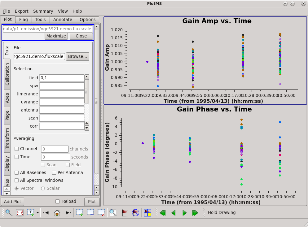
Now inspect the results of gaincal. The setup is identical to that used to plot the bandpass response curve. The only change is that we are plotting the gaintable ngc5921.demo.gcal, and we're looking at solutions for both of the calibrator sources. The results are shown at right.
#=====================================================================
#
# Now use plotcal to examine the gain solutions
#
print '--Plotcal (fluxscaled gains)--'
default('plotcal')
caltable = ftable
field = '0,1'
# Set up 2x1 panels - upper panel amp vs. time
subplot = 211
yaxis = 'amp'
# No output file yet (wait to plot next panel)
saveinputs('plotcal',prefix+'.plotcal.gscaled.amp.saved')
if scriptmode:
    showgui = True
else:
    showgui = False
plotcal()
#
# Set up 2x1 panels - lower panel phase vs. time
subplot = 212
yaxis = 'phase'
saveinputs('plotcal',prefix+'.plotcal.gscaled.phase.saved')
#
# The amp and phase coherence looks good
# Pause script if you are running in scriptmode
if scriptmode:
    # If you want to do this interactively and iterate over antenna, set
    #iteration = 'antenna'
    showgui = True
    plotcal()
    user_check=raw_input('Return to continue script\n')
else:
    # No GUI for this script
    showgui = False
    # Now send final plot to file in PNG format (via .png suffix)
    figfile = caltable + '.plotcal.png'
    plotcal()
Apply the Solutions
Next, apply the calibration solutions to the calibrators themselves, and finally transfer the calibration solutions by interpolation (or nearest-neighbor sampling) to the source. The relevant task is applycal, which fills out a new column of calibrated data in the measurement set without wiping out the raw data column. The application is identical to that used for continuum data, except that the bandpass table is also included in the calibration. To apply multiple calibrations at once, provide the gaintable parameter with a list of calibration tables, as follows.
gaintable = ['ngc5921.demo.gcal', 'ngc5921.demo.bcal']
In the script snippet below, the python global variables ftable and btable replace the full table names.
#=====================================================================
#
# Apply our calibration solutions to the data
# (This will put calibrated data into the CORRECTED_DATA column)
#
print '--ApplyCal--'
default('applycal')
vis = msfile
# We want to correct the calibrators using themselves
# and transfer from 1445+099 to itself and the target N5921
# Start with the fluxscale/gain and bandpass tables
gaintable = [ftable,btable]
# pick the 1445+099 out of the gain table for transfer
# use all of the bandpass table
gainfield = ['1','*']
# interpolation using linear for gain, nearest for bandpass
interp = ['linear','nearest']
# only one spw, do not need mapping
spwmap = []
# all channels
spw = ''
selectdata = False
# as before
gaincurve = False
opacity = 0.0
# select the fields for 1445+099 and N5921
field = '1,2'
applycal()
# Now for completeness apply 1331+305 to itself
field = '0'
gainfield = ['0','*']
# The CORRECTED_DATA column now contains the calibrated visibilities
saveinputs('applycal',prefix+'.applycal.saved')
# Pause script if you are running in scriptmode
if scriptmode:
    inp()
    user_check=raw_input('Return to continue script\n')
applycal()
Plot the Spectrum
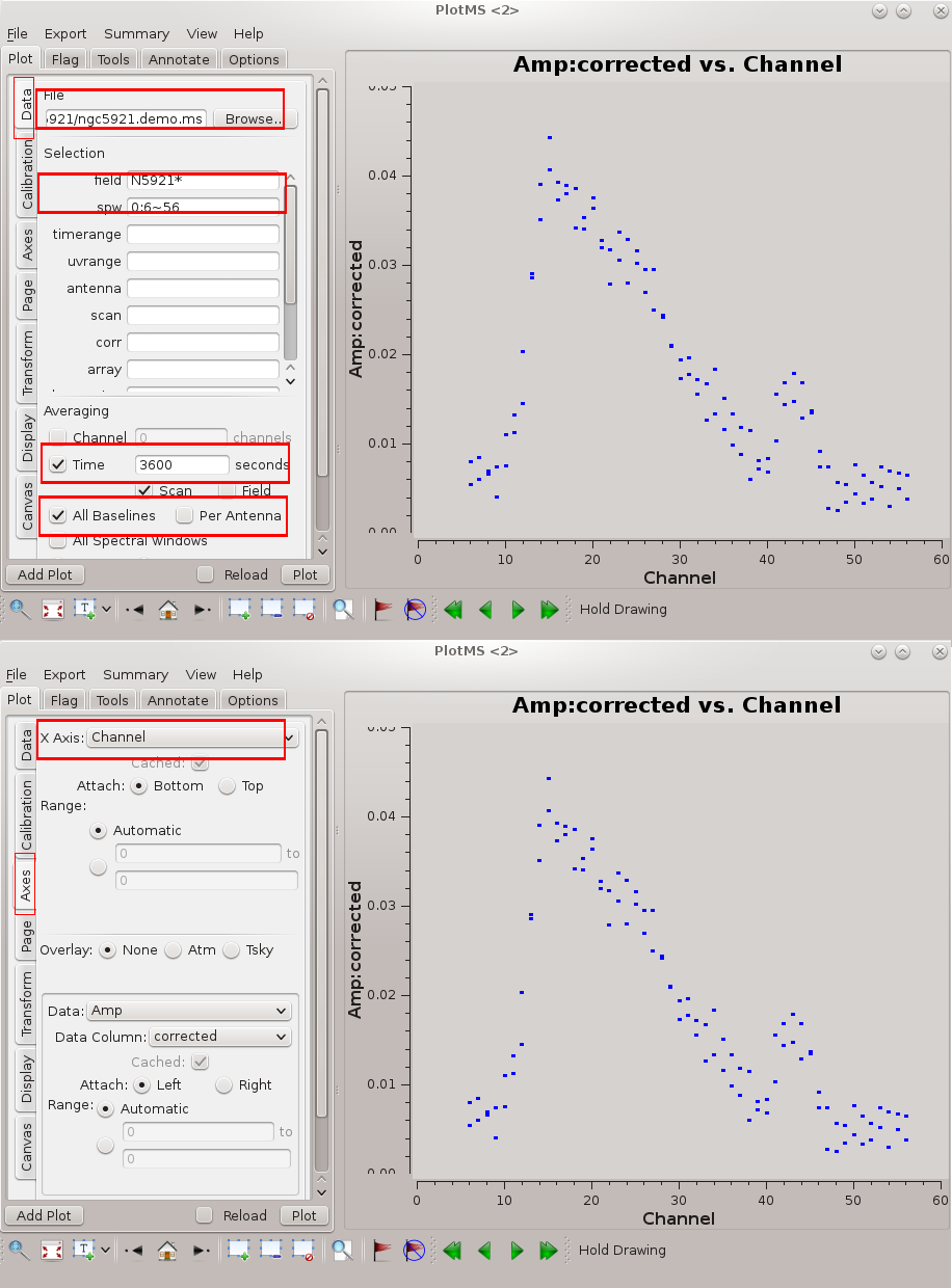
Before we attempt to image the 21 cm cube, we need to subtract off the underlying continuum, which means we need to plot the integrated spectrum of the source to determine the continuum channels.
We can do this in casaplotms.
#os.system("casaplotms")
The setup is illustrated in the figure at right. Briefly, we want to average both in time and over baselines to get the signal-to-noise necessary to reveal the 21 cm profile. Following the (Tab)Command convention of the flagging tutorial, here are the settings we need.
- (MS)field = N5921*
- (MS)spw = 0:6~56
- (MS)Averaging → Time = 3600 (average over some long time window)
- (MS)Averaging → All Baselines = True (checkmark)
- (Axes)X Axis = Channel
- (Axes)Y Axis = Amp
From inspection of this plot, it looks like channels 4~6 and 50~59 contain line-free channels, suitable to use for continuum subtraction.
Continuum Subtraction
The next step is to split off the NGC 5921 data from the multisource measurement set and subtract the continuum. Splitting uses the split command, as follows.
print '--Split NGC5921 Data--'
default('split')
vis = msfile
splitms = prefix + '.src.split.ms'
outputvis = splitms
field = 'N5921*'
spw = ''
datacolumn = 'corrected'
saveinputs('split',prefix+'.split.n5921.saved'
split()
print "Created "+splitms
This action generated a new measurement set called ngc5921.demo.src.split.ms and copied the calibrated source data (datacolumn = 'corrected') into it.
Uvcontsub subtracts the continuum from the data in the visibility (u, v) plane.
print '--UV Continuum Subtract--'
default('uvcontsub')
vis = splitms
field = 'N5921*'
# Use channels 4-6 and 50-59 for continuum
fitspw='0:4~6;50~59'
# Output all of spw 0
spw = '0'
# Averaging time (none)
solint = 0.0
# Fit only a mean level
fitorder = 0
# Do the uv-plane subtraction
fitmode = 'subtract'
# Let it split out the data automatically for us
splitdata = True
saveinputs('uvcontsub',prefix+'.uvcontsub.saved')
# Pause script if you are running in scriptmode
if scriptmode:
    inp()
    user_check=raw_input('Return to continue script\n')
uvcontsub()
Notice that uvcontsub splits two new measurement sets, 'ngc5921.demo.ms.cont', which contains an average of the continuum channels, and 'ngc5921.demo.ms.contsub', which contains the continuum-subtracted spectral line data.
Imaging
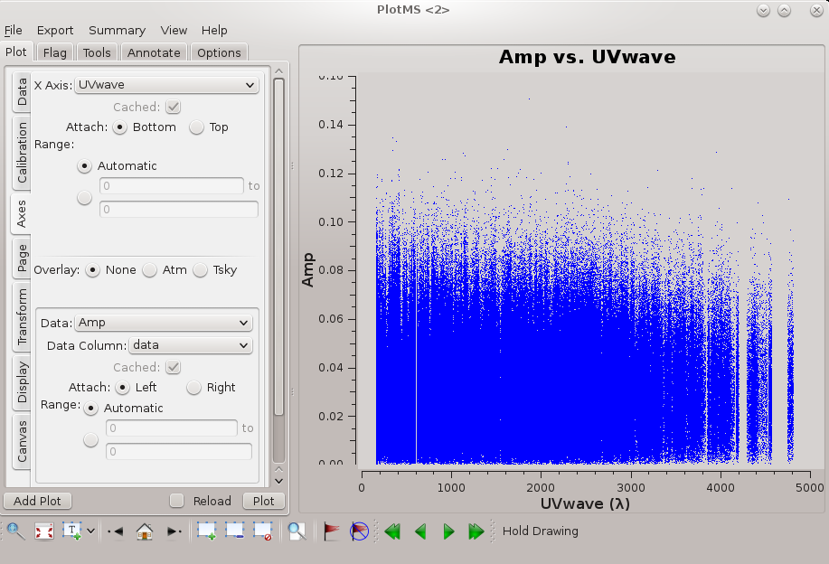
Now we can generate the primary science product, a CLEAN data cube (ra, dec, velocity) from the continuum-subtracted (u, v, channel) measurement set, ngc5921.demo.ms.contsub. Things to consider:
- To ensure channels aren't averaged prior to imaging, choose mode='channel'.
- Specify the channels to image using start = 5, width = 1 (no averaging over channels), nchan = 46; only channels 5~51 will be imaged.
- The maximum baseline is just under 5 kilolambda (see the figure at right), and so the expected synthetic beam is roughly 1.22 × 206265 / 5000 = 50 arcseconds. Pixels should sample the beam better than 3 times, so 15 arcseconds is a good choice of pixel size (cell = ['15.0arcsec','15.0arcsec']).
- We only want to clean down to the noise, which is easily determined by trial-and-error imaging of a single channel (choosing nchan=1 and start appropriately). Here, clean stops when the maximum residual on the channel is below threshold='8.0mJy'.
# identify the continuum subtracted measurement set
srcsplitms = splitms + '.contsub'
#=====================================================================
#
# Now clean an image cube of N5921
#
print '--Clean (clean)--'
default('clean')
# Pick up our split source continuum-subtracted data
vis = srcsplitms
# Make an image root file name
imname = prefix + '.cleanimg'
imagename = imname
# Set up the output image cube
mode = 'channel'
nchan = 46
start = 5
width = 1
# This is a single-source MS with one spw
field = '0'
spw = ''
# Standard gain factor 0.1
gain = 0.1
# Set the output image size and cell size (arcsec)
imsize = [256,256]
# Do a simple Clark clean
psfmode = 'clark'
# No Cotton-Schwab iterations
csclean = False
# Pixel size 15 arcsec for this data (1/3 of 45" beam)
# VLA D-config L-band
cell = ['15.0arcsec','15.0arcsec']
# Fix maximum number of iterations
niter = 6000
# Also set flux residual threshold (in mJy)
threshold='8.0mJy'
# Set up the weighting
# Use Briggs weighting (a moderate value, on the uniform side)
weighting = 'briggs'
robust = 0.5
# Set a cleanbox +/-20 pixels around the center 128,128
mask = [108,108,148,148]
# If you want interactive clean set to True
#interactive=True
interactive=False
saveinputs('clean',prefix+'.clean.saved')
# Pause script if you are running in scriptmode
if scriptmode:
    inp()
    user_check=raw_input('Return to continue script\n')
clean()
Additional Science Products
If things went well, you should now have a spectral line cube (ngc5921.demo.cleanimg.img) as a primary science product. The demo script illustrates further how to generate cube statistics (using imstat), an integrated spectrum, and moment maps.
The Integrated Spectrum
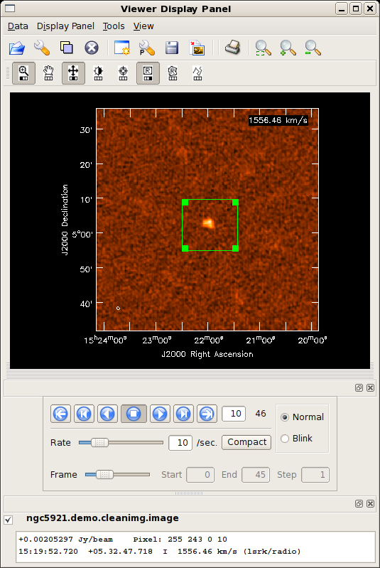
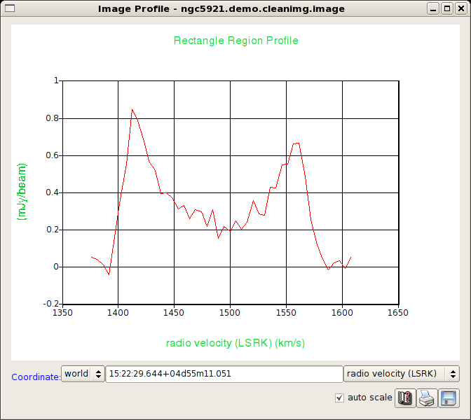
We saw earlier how to generate an integrated spectrum from the (u, v) measurement set. Here's how to produce the integrated spectrum from the spectral line cube. First, load the cube into viewer.
# Store the name of the clean image into a python global
clnimage = imname+'.image'
#if you are performing the operations interactively, you can lose the scriptmode commands.
# viewer(clnimage, 'image') at the casapy command prompt would suffice.
if scriptmode:
    print '--View image--'
    print "Use Spectral Profile Tool to get line profile in box in center"
    viewer(clnimage,'image')
    user_check=raw_input('Return to continue script\n')
To generate the integrated spectrum, perform the following tasks.
- Use the player controls
 to inspect the cube one channel at a time.
 - From the viewer Tools menu, select Spectral Profile. A new graphics window should appear.
- By default, the rectangle selection tool
 is assigned to the right mouse button, and you can just right-click and drag a box over the region where you want to (spatially) integrate the spectrum. See the figure at upper right.
 - Alternatively, you can assign one of the other selection tools by right-clicking on the appropriate button.
- The spectrum now appears in the graphics window; see the figure at lower right.
You can save the integrated spectrum to a text file by clicking the ![]() button on the graphics window. There are also buttons to print the figure or save the figure to disk.
button on the graphics window. There are also buttons to print the figure or save the figure to disk.
Export the Cube
Work in progress!
Appendix: Python Notes
os.system
os.system allows you to run shell commands from within python / CASA. For example:
import os
os.system('ls -sF')
will give an OS-level listing of the current directory's contents.
os.environ.get
It's worth having a look at the output of the os.environ.get command to understand the python syntax (alternative: os.getenv). You can think of os.environ as a list of operating system environment variables, and get is a method that extracts information about the requested environment variable, here, CASAPATH. Get returns a string of whitespace separated information, and .split() turns that string into a list. The array index [0] extracts the first element of that list, which contains the path.
To illustrate, here is some example python I/O in CASA.
CASA <12>: print os.environ.get('CASAPATH')
/usr/lib64/casapy/30.0.9709test-001 linux local el5bld64b

CASA <13>: print os.environ.get('CASAPATH').split()
['/usr/lib64/casapy/30.0.9709test-001', 'linux', 'local', 'el5bld64b']

CASA <14>: print os.environ.get('CASAPATH').split()[0]
/usr/lib64/casapy/30.0.9709test-001
--Jack Gallimore 16:58, 7 December 2009 (UTC)