Antennae Band7 - Calibration for CASA 3.3: Difference between revisions
| Line 418: | Line 418: | ||
==Bandpass and gain calibration== | ==Bandpass and gain calibration== | ||
Next we | Next we plot the phase as a function of time and frequency for the bandpass calibrator, 3c279. For the first plot, Figure 7, we use avgscan=T and avgtime='1e8' to average in time over all scans and integrations, and we specify coloraxis='baseline' to colorize by baseline. For the second, Figure 8, we use spw='0:40~3800' and avgchannel='3840' to average over the central channels of the first spectral window. For both plots we will iterate on antenna (interaxis='antenna'). Use the green arrows of the plotms GUI to view the plots for different antennas. | ||
[[File:Uid_A002_X1ff7b0_Xb- | [[File:Uid_A002_X1ff7b0_Xb-phasecont.png|200px|thumb|right|Fig. 7. Phase vs. time for the phase calibrator, 3c279. Averaged over channel. Only baselines with antenna DV02, and corr='XX']] | ||
[[File:Uid_A002_X1ff7b0_Xb- | [[File:Uid_A002_X1ff7b0_Xb-bandpass.png|200px|thumb|right|Fig. 8. Phase vs. frequency for the phase calibrator, 3c279. Averaged over time, and corr='XX']] | ||
<source lang="python"> | <source lang="python"> | ||
| Line 428: | Line 428: | ||
xaxis='freq', yaxis='phase', | xaxis='freq', yaxis='phase', | ||
selectdata=True, field='3c279', corr='XX', antenna='*&*', | selectdata=True, field='3c279', corr='XX', antenna='*&*', | ||
avgtime=' | avgtime='1e8', avgscan=T, | ||
coloraxis='baseline', iteraxis='antenna') | coloraxis='baseline', iteraxis='antenna') | ||
</source> | </source> | ||
| Line 441: | Line 441: | ||
</source> | </source> | ||
Figure 7 shows that the phase variation as function of time, although smoothly varying, will need to be calibrated in order to obtain proper bandpass solutions. In Figure 8 we see that phase variations in dataset uid_A002_X1ff7b0_Xb are small, typically ~ 30 degrees. | |||
We issue {{gaincal}} on 3c279 to determine phase(-only) gain solutions. We will use solint='int' for the solution interval, which means that one gain solution will be determined for every integration time. This short integration time is possible because the bandpass calibrator is a very bright point source, so we have very high signal-to-noise and a perfect model. This will correct for any phase variations in the bandpass calibrator as a function of time, a step which will prevent decorrelation of the vector-averaged bandpass solutions. We will then apply these solutions on-the-fly when we run {{bandpass}}. | |||
We will use the average of channels 40~3800 and two spw to increase our signal-to-noise in the determination of the antenna-based phase solutions. Averaging over a subset of channels near the center of the bandpass is acceptable when the phase variation as a function of channel is small. For our reference antenna, we choose DV06. We call the output calibration table asdm+'.g1.cal'. | We will use the average of channels 40~3800 and two spw to increase our signal-to-noise in the determination of the antenna-based phase solutions. Averaging over a subset of channels near the center of the bandpass is acceptable when the phase variation as a function of channel is small. For our reference antenna, we choose DV06. We call the output calibration table asdm+'.g1.cal'. | ||
Revision as of 05:54, 21 July 2011
Overview
This portion of the AntennaeBand7 CASA Guide will cover the calibration of the raw visibility data. To skip to the imaging portion of the guide, see: Antennae Band7 - Imaging.
If you haven't already downloaded the raw data, you may do that now by clicking on the region closest to your location and downloading the file named 'Antennae_Band7_UnCalibratedMSandTablesForReduction.tgz':
Once the download has finished, unpack the file:
# In a terminal outside CASA
tar -xvzf Antennae_Band7_UnCalibratedMSandTablesForReduction.tgz

cd Antennae_Band7_UnCalibratedMSandTablesForReduction

# Start CASA
casapy
The data have already been converted to CASA Measurement Set (MS) format using the CASA task importasdm. Accompanying the data are some basic calibration tables you will need for the following reduction, as well as the *.ms.flagversions files that are automatically generated by importasdm.
Initial Inspection
We will eventually concatenate the nine datasets used here into one large dataset. However, we will keep them separate for now, as some of the steps to follow require individual datasets (specifically, the application of the Tsys and WVR tables). We therefore start by defining an array "basename_all" that includes the names of the six files in chronological order. This will simplify the following steps by allowing us to loop through the files using a simple for-loop in python. Remember that if you log out of CASA, you will have to re-issue this command. We will remind you of this in the relevant sections by repeating the command at the start.
# In CASA
basename_all=["uid___A002_X1ff7b0_Xb","uid___A002_X207fe4_X3a","uid___A002_X207fe4_X3b9",
     "uid___A002_X2181fb_X49","uid___A002_X1ff7b0_X1c8","uid___A002_X207fe4_X1f7",
     "uid___A002_X207fe4_X4d7","uid___A002_X215db8_X18","uid___A002_X215db8_X1d5",
     "uid___A002_X215db8_X392"]
The usual first step is then to get some basic information about the data. We do this using the task listobs, which will output a detailed summary of each dataset supplied.
# In CASA
for name in basename_all:
        listobs(vis=name+'.ms')
Note that after cutting and pasting a for-loop you often have to press return several times to execute. The output will be sent to the CASA logger. You will have to scroll up to see the individual output for each of the datasets. Here is an example of the output for first dataset in the list, uid___A002_X1ff7b0_Xb.ms (northern mosaic).
2011-07-21 02:50:25 INFO PlotMS	================================================================================
2011-07-21 02:50:25 INFO PlotMS          MeasurementSet Name:
 /Users/despada/Desktop/Imaging/Antennae/Datasets/band7/uid___A002_X1ff7b0_Xb.ms      MS Version 2
2011-07-21 02:50:25 INFO PlotMS	================================================================================
2011-07-21 02:50:25 INFO PlotMS	   Observer: Unknown     Project: T.B.D.
2011-07-21 02:50:25 INFO PlotMS	Observation: ALMA(11 antennas)
2011-07-21 02:50:25 INFO PlotMS	Data records: 181357       Total integration time = 4931.71 seconds
2011-07-21 02:50:25 INFO PlotMS	   Observed from   28-May-2011/01:25:27.6   to   28-May-2011/02:47:39.3 (UTC)
2011-07-21 02:50:25 INFO PlotMS	Fields: 26
2011-07-21 02:50:25 INFO PlotMS	  ID   Code Name         RA            Decl           Epoch   SrcId
2011-07-21 02:50:25 INFO PlotMS	  0    none 3c279        12:56:11.1666 -05.47.21.5247 J2000   0
2011-07-21 02:50:25 INFO PlotMS	  1    none Titan        12:42:43.9481 -01.43.38.3190 J2000   1
2011-07-21 02:50:25 INFO PlotMS	  2    none NGC4038 - A* 12:01:53.1701 -18.52.37.9200 J2000   2
2011-07-21 02:50:25 INFO PlotMS	  3    none NGC4038 - A* 12:01:51.9030 -18.51.49.9437 J2000   2
2011-07-21 02:50:25 INFO PlotMS	  4    none NGC4038 - A* 12:01:52.4309 -18.51.49.9437 J2000   2
2011-07-21 02:50:25 INFO PlotMS	  5    none NGC4038 - A* 12:01:52.9587 -18.51.49.9437 J2000   2
2011-07-21 02:50:25 INFO PlotMS	  6    none NGC4038 - A* 12:01:53.4866 -18.51.49.9436 J2000   2
2011-07-21 02:50:25 INFO PlotMS	  7    none NGC4038 - A* 12:01:54.0144 -18.51.49.9436 J2000   2
2011-07-21 02:50:25 INFO PlotMS	  8    none NGC4038 - A* 12:01:52.1669 -18.51.56.4319 J2000   2
2011-07-21 02:50:25 INFO PlotMS	  9    none NGC4038 - A* 12:01:52.6948 -18.51.56.4318 J2000   2
2011-07-21 02:50:25 INFO PlotMS	  10   none NGC4038 - A* 12:01:53.2226 -18.51.56.4318 J2000   2
2011-07-21 02:50:25 INFO PlotMS	  11   none NGC4038 - A* 12:01:53.7505 -18.51.56.4318 J2000   2
2011-07-21 02:50:25 INFO PlotMS	  12   none NGC4038 - A* 12:01:51.9030 -18.52.02.9201 J2000   2
2011-07-21 02:50:25 INFO PlotMS	  13   none NGC4038 - A* 12:01:52.4309 -18.52.02.9200 J2000   2
2011-07-21 02:50:25 INFO PlotMS	  14   none NGC4038 - A* 12:01:52.9587 -18.52.02.9200 J2000   2
2011-07-21 02:50:25 INFO PlotMS	  15   none NGC4038 - A* 12:01:53.4866 -18.52.02.9200 J2000   2
2011-07-21 02:50:25 INFO PlotMS	  16   none NGC4038 - A* 12:01:54.0144 -18.52.02.9199 J2000   2
2011-07-21 02:50:25 INFO PlotMS	  17   none NGC4038 - A* 12:01:52.1669 -18.52.09.4082 J2000   2
2011-07-21 02:50:25 INFO PlotMS	  18   none NGC4038 - A* 12:01:52.6948 -18.52.09.4082 J2000   2
2011-07-21 02:50:25 INFO PlotMS	  19   none NGC4038 - A* 12:01:53.2226 -18.52.09.4082 J2000   2
2011-07-21 02:50:25 INFO PlotMS	  20   none NGC4038 - A* 12:01:53.7505 -18.52.09.4081 J2000   2
2011-07-21 02:50:25 INFO PlotMS	  21   none NGC4038 - A* 12:01:51.9030 -18.52.15.8964 J2000   2
2011-07-21 02:50:25 INFO PlotMS	  22   none NGC4038 - A* 12:01:52.4309 -18.52.15.8964 J2000   2
2011-07-21 02:50:25 INFO PlotMS	  23   none NGC4038 - A* 12:01:52.9587 -18.52.15.8963 J2000   2
2011-07-21 02:50:25 INFO PlotMS	  24   none NGC4038 - A* 12:01:53.4866 -18.52.15.8963 J2000   2
2011-07-21 02:50:25 INFO PlotMS	  25   none NGC4038 - A* 12:01:54.0144 -18.52.15.8963 J2000   2
2011-07-21 02:50:25 INFO PlotMS	   (nVis = Total number of time/baseline visibilities per field)
2011-07-21 02:50:25 INFO PlotMS	Spectral Windows:  (9 unique spectral windows and 2 unique polarization setups)
2011-07-21 02:50:25 INFO PlotMS	  SpwID  #Chans Frame Ch1(MHz)    ChanWid(kHz)TotBW(kHz)  Ref(MHz)    Corrs
2011-07-21 02:50:25 INFO PlotMS	  0           4 TOPO  184550      1500000     7500000     183300      I
2011-07-21 02:50:25 INFO PlotMS	  1        3840 TOPO  344845.586  488.28125   1875000     344908.33   XX  YY
2011-07-21 02:50:25 INFO PlotMS	  2           1 TOPO  343908.086  1875000     1875000     344908.33   XX  YY
2011-07-21 02:50:25 INFO PlotMS	  3        3840 TOPO  356845.586  488.28125   1875000     344908.33   XX  YY
2011-07-21 02:50:25 INFO PlotMS	  4           1 TOPO  343908.086  1875000     1875000     344908.33   XX  YY
2011-07-21 02:50:25 INFO PlotMS	  5         128 TOPO  344900.518  15625       2000000     344908.33   XX  YY
2011-07-21 02:50:25 INFO PlotMS	  6           1 TOPO  343892.705  1796875     1796875     344908.33   XX  YY
2011-07-21 02:50:25 INFO PlotMS	  7         128 TOPO  356900.518  15625       2000000     344908.33   XX  YY
2011-07-21 02:50:25 INFO PlotMS	  8           1 TOPO  343892.705  1796875     1796875     344908.33   XX  YY
2011-07-21 02:50:25 INFO PlotMS	Sources: 60
2011-07-21 02:50:25 INFO PlotMS	  ID   Name         SpwId RestFreq(MHz)  SysVel(km/s)
2011-07-21 02:50:25 INFO PlotMS	  0    3c279        0     -              -
2011-07-21 02:50:25 INFO PlotMS	  0    3c279        9     -              -
2011-07-21 02:50:25 INFO PlotMS	  0    3c279        10    -              -
2011-07-21 02:50:25 INFO PlotMS	  0    3c279        11    -              -
2011-07-21 02:50:25 INFO PlotMS	  0    3c279        12    -              -
2011-07-21 02:50:25 INFO PlotMS	  0    3c279        13    -              -
2011-07-21 02:50:25 INFO PlotMS	  0    3c279        14    -              -
2011-07-21 02:50:25 INFO PlotMS	  0    3c279        15    -              -
2011-07-21 02:50:25 INFO PlotMS	  0    3c279        16    -              -
2011-07-21 02:50:25 INFO PlotMS	  0    3c279        17    -              -
2011-07-21 02:50:25 INFO PlotMS	  0    3c279        18    -              -
2011-07-21 02:50:25 INFO PlotMS	  0    3c279        19    -              -
2011-07-21 02:50:25 INFO PlotMS	  0    3c279        1     -              -
2011-07-21 02:50:25 INFO PlotMS	  0    3c279        2     -              -
2011-07-21 02:50:25 INFO PlotMS	  0    3c279        3     -              -
2011-07-21 02:50:25 INFO PlotMS	  0    3c279        4     -              -
2011-07-21 02:50:25 INFO PlotMS	  1    Titan        0     -              -
2011-07-21 02:50:25 INFO PlotMS	  1    Titan        9     -              -
2011-07-21 02:50:25 INFO PlotMS	  1    Titan        10    -              -
2011-07-21 02:50:25 INFO PlotMS	  1    Titan        11    -              -
2011-07-21 02:50:25 INFO PlotMS	  1    Titan        12    -              -
2011-07-21 02:50:25 INFO PlotMS	  1    Titan        13    -              -
2011-07-21 02:50:25 INFO PlotMS	  1    Titan        14    -              -
2011-07-21 02:50:25 INFO PlotMS	  1    Titan        15    -              -
2011-07-21 02:50:25 INFO PlotMS	  1    Titan        16    -              -
2011-07-21 02:50:25 INFO PlotMS	  1    Titan        17    -              -
2011-07-21 02:50:25 INFO PlotMS	  1    Titan        18    -              -
2011-07-21 02:50:25 INFO PlotMS	  1    Titan        19    -              -
2011-07-21 02:50:25 INFO PlotMS	  1    Titan        1     -              -
2011-07-21 02:50:25 INFO PlotMS	  1    Titan        2     -              -
2011-07-21 02:50:25 INFO PlotMS	  1    Titan        3     -              -
2011-07-21 02:50:25 INFO PlotMS	  1    Titan        4     -              -
2011-07-21 02:50:25 INFO PlotMS	  0    Titan        5     -              -
2011-07-21 02:50:25 INFO PlotMS	  0    Titan        6     -              -
2011-07-21 02:50:25 INFO PlotMS	  0    Titan        7     -              -
2011-07-21 02:50:25 INFO PlotMS	  0    Titan        8     -              -
2011-07-21 02:50:25 INFO PlotMS	  1    3c279        5     -              -
2011-07-21 02:50:25 INFO PlotMS	  1    3c279        6     -              -
2011-07-21 02:50:25 INFO PlotMS	  1    3c279        7     -              -
2011-07-21 02:50:25 INFO PlotMS	  1    3c279        8     -              -
2011-07-21 02:50:25 INFO PlotMS	  2    NGC4038 - A* 0     -              -
2011-07-21 02:50:25 INFO PlotMS	  2    NGC4038 - A* 9     -              -
2011-07-21 02:50:25 INFO PlotMS	  2    NGC4038 - A* 10    -              -
2011-07-21 02:50:25 INFO PlotMS	  2    NGC4038 - A* 11    -              -
2011-07-21 02:50:25 INFO PlotMS	  2    NGC4038 - A* 12    -              -
2011-07-21 02:50:25 INFO PlotMS	  2    NGC4038 - A* 13    -              -
2011-07-21 02:50:25 INFO PlotMS	  2    NGC4038 - A* 14    -              -
2011-07-21 02:50:25 INFO PlotMS	  2    NGC4038 - A* 15    -              -
2011-07-21 02:50:25 INFO PlotMS	  2    NGC4038 - A* 16    -              -
2011-07-21 02:50:25 INFO PlotMS	  2    NGC4038 - A* 17    -              -
2011-07-21 02:50:25 INFO PlotMS	  2    NGC4038 - A* 18    -              -
2011-07-21 02:50:25 INFO PlotMS	  2    NGC4038 - A* 19    -              -
2011-07-21 02:50:25 INFO PlotMS	  2    NGC4038 - A* 1     -              -
2011-07-21 02:50:25 INFO PlotMS	  2    NGC4038 - A* 2     -              -
2011-07-21 02:50:25 INFO PlotMS	  2    NGC4038 - A* 3     -              -
2011-07-21 02:50:25 INFO PlotMS	  2    NGC4038 - A* 4     -              -
2011-07-21 02:50:25 INFO PlotMS	  2    NGC4038 - A* 5     -              -
2011-07-21 02:50:25 INFO PlotMS	  2    NGC4038 - A* 6     -              -
2011-07-21 02:50:25 INFO PlotMS	  2    NGC4038 - A* 7     -              -
2011-07-21 02:50:25 INFO PlotMS	  2    NGC4038 - A* 8     -              -
2011-07-21 02:50:25 INFO PlotMS	Antennas: 11 'name'='station'
2011-07-21 02:50:25 INFO PlotMS	   ID=   0-3: 'DV02'='A015', 'DV04'='J505', 'DV06'='T704', 'DV07'='A004',
2011-07-21 02:50:25 INFO PlotMS	   ID=   4-7: 'DV08'='A072', 'DV09'='A008', 'DV10'='A009', 'DV11'='A016',
2011-07-21 02:50:25 INFO PlotMS	   ID=  8-10: 'PM01'='T702', 'PM02'='A017', 'PM03'='J504'
================================================================================
This output shows that three fields were observed: 3c279, Titan, and the different pointing of the Antennae mosaic (NGC 4038 in this case). Field 0 (3c279) will serve as the gain calibrator and bandpass calibrator; field 1 (Titan) will serve as the flux calibrator; and source id 2 (NGC 4038) is, of course, the science target. Note that the source id 2 is composed of a number of field ids, each corresponding to a different pointing in the mosaic. In particular, the observations are characterized by 23 pointings for the Northern mosaic (NGC 4038), and 29 pointings for the Southern mosaic (NGC 4039).
Note that there are more than two SpwIDs even though the observations were set up to have two spectral windows. The spectral line data themselves are found in spectral windows 1,3, which have 3840 channels each. The first one (spw 1) is centered on the CO(3-2) emission line in the Antennae. There is one additional spectral window (spw 3) in the Upper Side Band (USB). The additional spectral window is used to measure the continuum emission in the galaxy, and may contain other emission lines as well. The spectral resolution and total bandwidth of these two spectral windows are 488.28 MHz and 1.875 GHz (3840 channels), respectively, corresponding to 0.426 km/s and 1634 km/s. There are two spectral windows (spw 5 and 7) fully covering spw 1 and 3 but in TDM mode (2 GHz bandwidth, 128 channels), which are used for tsys calibration.
Spectral windows 2,4,6,8 contain channel averages of the data in spectral windows 1,3,5,7, respectively. These are not useful for the offline data reduction. Spectral window 0 contains the WVR data. You may notice that there are additional SpwIDs listed in the "Sources" section which are not listed in the "Spectral Windows" section. These spectral windows are reserved for the WVRs of each antenna (seven in our case). At the moment, all WVRs point to spw 0, which contains nominal frequencies. The additional spectral windows (spw 9-15) are therefore not used and can be ignored.
Another important thing to note is that the position of Titan is listed as 00:00:00.0000 +00.00.00.0000. This is due to the fact that for ephemeris objects, the positions are currently not stored in the asdm. This will be handled correctly in the near future, but at present, we have to fix this offline. We will correct the coordinates below by running the procedure fixplanets, which takes the position from the pointing table.
The final column of the listobs output in the logger (not shown above) gives the scan intent. This information is used later to flag the pointing scans and the hot and ambient load calibration scans, using scan intent as a selection option. Also these intents will be used in the future for pipeline processing.
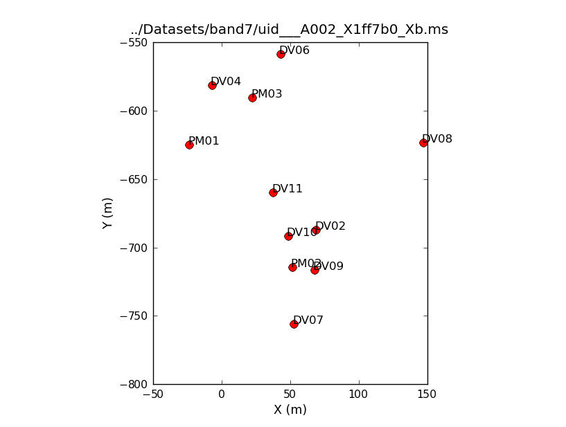
A total of 11 antennas were used for the dataset listed above. Note that numbering in python always begins with "0", so the antennas have IDs 0-10. To see what the antenna configuration looked like at the time of this observation, we will use the task plotants (Figure 1).
# In CASA
plotants(vis=basename[0]+'.ms', figfile=basename[0]+'_plotants.png')
This will plot the antenna configuration on your screen as well as save it under the specified filename for future reference. You can check using plotants for the other datasets that the configuration stays relatively constant during the course of the observations.
No large phase delays are found in any of the datasets (i.e., usually less than one wrap over the bandpass), so bandpass calibration should remove this effect properly.
Data edition
General flagging
The first editing we will do is some a priori flagging with flagdata and flagautocorr. We will start by flagging the shadowed data and the autocorrelation data. ALMA data contains both the cross correlation and autocorrelation data, but here we are only interested in the cross-correlation data. Additionally, for compact configurations of the array, one antenna can shadow another, blocking its view. These data also need to be flagged. Remember that you first need to redefine the "basename" array if you logged out of CASA prior to starting this subsection.
# In CASA
basename_all=["uid___A002_X1ff7b0_Xb","uid___A002_X1ff7b0_X1c8","uid___A002_X207fe4_X3a",
                          "uid___A002_X207fe4_X1f7","uid___A002_X207fe4_X3b9","uid___A002_X207fe4_X4d7",
                          "uid___A002_X215db8_X18","uid___A002_X215db8_X1d5","uid___A002_X215db8_X392",
                          "uid___A002_X2181fb_X49"]
Now we will loop over the datasets, running the two flagging commands:
# In CASA
for asdm in basename_all:
	flagdata(vis=asdm+'.ms', flagbackup = F, mode = 'shadow')
	flagautocorr(vis=asdm+'.ms')
There are a number of scans in the data that were used for pointing and atmospheric (i.e. Tsys) calibration, and are no longer needed. We can flag them using flagdata by selecting them on the 'intent' keyword:
# In CASA
for asdm in basename_all:
        flagdata(vis=asdm+'.ms', mode='manualflag', flagbackup = F, intent='*POINTING*')
        flagdata(vis=name+'.ms', mode='manualflag', flagbackup = F, intent='*ATMOSPHERE*')
Next we store the current flagging information for each dataset using the flagmanager:
# In CASA
for name in basename:
        flagmanager(vis = name+'.ms', mode = 'save', versionname = 'Apriori')
Apply WVR and Tsys calibration tables
First, remember to re-define the "basename_all" array if you have logged out of CASA at any point up until now during the data edition process.
# In CASA
basename_all=["uid___A002_X1ff7b0_Xb","uid___A002_X1ff7b0_X1c8","uid___A002_X207fe4_X3a",
                          "uid___A002_X207fe4_X1f7","uid___A002_X207fe4_X3b9","uid___A002_X207fe4_X4d7",
                          "uid___A002_X215db8_X18","uid___A002_X215db8_X1d5","uid___A002_X215db8_X392",
                           "uid___A002_X2181fb_X49"]
Tsys tables
ALMA does not automatically scale the data by system temperature (Tsys) as would be done at other radio telescopes. Tsys measurements correct for the atmospheric opacity (to first-order), both as a function of time and as a function of frequency, and put weights in the subsequent imaging. The Tsys tables for these datasets were provided with the downloadable data. The FDM Tsys table has been obtained using that of the TDM mode spectral window (2 GHz, 128 channels per baseband, XX and YY polarizations), which we interpolated to have tsys data for all the FDM channels (3840 channels per baseband, XX and YY polarizations, over 1.875 GHz).
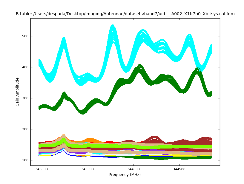
We inspect the Tsys tables for spw=1 with the task plotcal, for example for the first dataset:
asdm=basename_all[0]
plotcal(caltable=asdm+'.tsys.cal.fdm',
             xaxis="freq",yaxis="amp",
             timerange='<1e8',spw='1'
              overplot=False,plotrange=[0, 0, 0, 0],plotsymbol=".")
In Figure 2 we show the Tsys for all the antennas. The Tsys solutions look reliable, except for one antenna that shows large values of Tsys (DV04, 2 polarizations per baseband). We will flag that antenna. Also note that there is an absorption line at about 345.2 GHz that makes Tsys larger, as seen in all of the other antennas.
Apply Tsys and WVR tables
We will now apply the Tsys and the WVR calibration tables to the data with the task applycal. We do this for each field separately so that the appropriate calibration data are applied to the right fields. The "field" parameter specifies the field to which we will apply the calibration, and the "gainfield" parameter specifies the field from which we wish to take the calibration solutions from the gaintable. In the call to applycal, we will specify interpolation="nearest". Now loop through the datasets as described above, applying the Tsys and WVR calibration tables to all the datasets and sources:
We will apply the calibration tables with applycal:
# In CASA
for asdm in basename_all:
	for fieldname in ['Titan','3c279','NGC4038*','Antenna*']:
		applycal(vis=asdm+".ms", spw='1,3', flagbackup=F,
                                field=fieldname, gainfield=fieldname,
                                interp=['nearest','nearest'],
                                 gaintable=[asdm+".tsys.cal.fdm",asdm+'.wvr.cal'])
Now you can use plotms to show some of the before-and-after effects of calibration. Just re-run the previous plotms command, repeated below, or if the window is still open, check 'force reload'. This will display the uncorrected phases across the band. To display the corrected phases, you will need to select the 'corrected' in the 'Data Column' field of the 'Axes' tab of plotms and re-plot.
# In CASA
plotms(vis=basename[0]+'.ms',
              field='3c279'
              xaxis='channel', yaxis='phase',
              selectdata=T, spw='1', correlation='XX',
              avgtime='1e8',avgscan=T,
              coloraxis='baseline' )
Additional individual flagging
Continuum plot
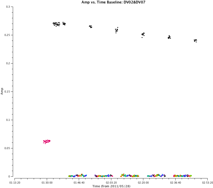
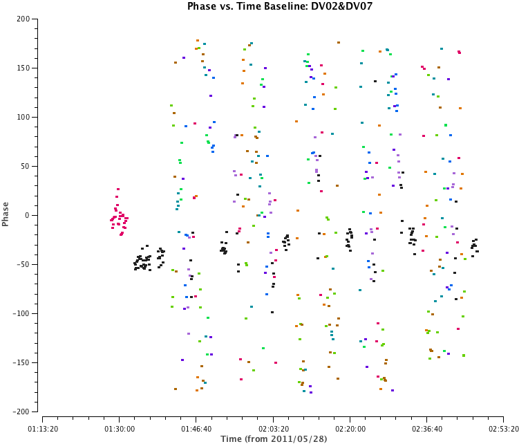
Next we will do some additional inspection with plotms. First we will plot amplitude versus time (see Figure 3), averaging over all channels of spectral window 1 (spw = 1, where the CO(3-2) line is) and colorizing by field, for example for the first dataset. Scans on Titan are colored red, the bandpass and phase calibrator 3c279 is colored black, and the different pointings of the Antennae mosaic in different colors. Figure 4 shows the phase versus time plot, with the same color.
Check carefully that the amplitudes and phases vary smoothly with time. The Tsys corrected data should have approximately constant amplitudes and the WVR corrected data should usually have lower phase scatter. Note that the amplitudes in Figure 3 are decreasing, as a result of the decreasing elevation of the source. The Tsys corrected data (choose 'corrected' in Axes > Data Column in plotms) show constant amplitudes.
These are the plotms instances to produce the continuum plots:
# In CASA

asdm=basename_all[0]

plotms(vis=asdm+'.ms',
            xaxis='time', yaxis='amp',
            selectdata=True, spw='1', correlation='XX',antenna='*&*',
            avgchannel='3840', avgscan=T,
            iteraxis='baseline',coloraxis='field')

plotms(vis=asdm+'.ms',
            xaxis='time', yaxis='phase',
            selectdata=True, spw='1', correlation='XX',antenna='*&*',
            avgchannel='3840', avgscan=T,
            iteraxis='baseline',coloraxis='field')
where:
- xaxis='time', yaxis='X' : a plot of X (amplitude or phase) versus time.
- avgchannel='3840' : average over all the channels in the spectral window.
- spw='1', correlation='XX',antenna='*&*': Select only the spectral window 1, polarization XX and cross-correlation data.
- iteraxis='baseline',coloraxis='field': Iterate over baseline, and colorize by different fields.
Select correlation='YY' to inspect the other polarization.
Spectral plot
Second we plot the amplitude and phase versus frequency for the two correlations, XX and YY. Figure 5 and 6 show an example of spectral plot for the bandpass and phase calibrator 3c279, for both correlations. Again, since this source is a quasar, the amplitudes should be constant (Tsys corrected) and phases varying smoothly.
These are the task instances to obtain these plots:
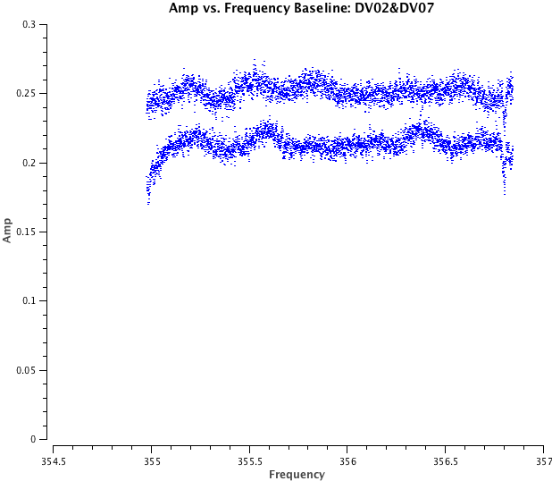
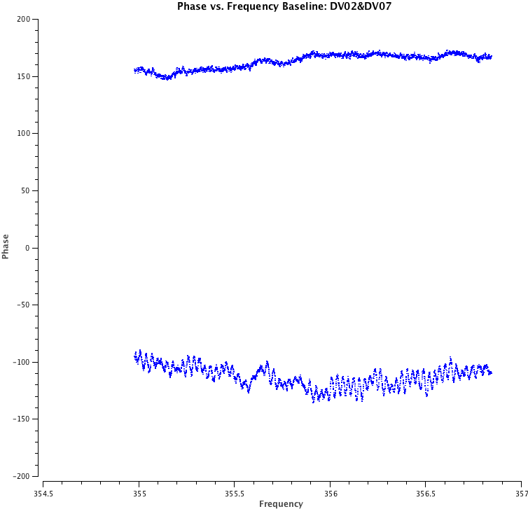
# In CASA
plotms(vis = asdm+'.split.ms',
             xaxis = 'frequency',yaxis = 'phase',
             field='3c279'
             avgtime = '1e8',avgscan = T,
             selectdata=True, antenna = '*&*',
             iteraxis='baseline')

plotms(vis = asdm+'.split.ms',
             xaxis = 'frequency',yaxis = 'amp',
             field='3c279'
             avgtime = '1e8',avgscan = T,
             selectdata=True, antenna = '*&*',
             iteraxis='baseline')
where:
- xaxis = 'frequency',yaxis = 'X': plot X (amplitude or phase) versus frequency
- field = '3c279': plot only our bandpass and phase calibrator
- avgtime = '1e8',avgscan = T: average all scans and integrations
- antenna = '*&*: plot only cross-correlation data
- iteraxis='baseline': iterate for each baseline
You can plot other sources as well. By selecting any pointing of Antennae, you should be able to see clearly the (still uncalibrated) CO(3-2) line.
The flux calibrator also present some emission line in this spectral window.
Individual Flagging
First we use flagdata to remove the edge channels from both sides of the bandpass:
# In CASA
flagdata(flagbackup = F,vis = asdm+'.split.ms',spw = '1:0~7,1:3831~3839')
Continue to inspect the data with plotms, plotting different axes and colorizing by the different parameters. Don't forget to average the data if possible to speed the plotting process. The time ranges to insert in flagdata can be obtained using plotms Tools Hover/Display. Instead of using the following flagdata commands, you can also flag by hand in plotms. To do this, select your bad data by clicking on the 'Mark Regions" button, then on 'Flag".
File:AntennaeDataInspection-Band7.txt contains the different problems that have been identified for all the datasets. We indicated how to flag the bad data in different instances of the flagdata command. For example, for the first dataset:
asdm="uid___A002_X1ff7b0_Xb"
#0-3: 'DV02'='A015', 'DV04'='J505', 'DV06'='T704', 'DV07'='A004',
#4-7: 'DV08'='A072', 'DV09'='A008', 'DV10'='A009', 'DV11'='A016',
#8-10: 'PM01'='T702', 'PM02'='A017', 'PM03'='J504'
#Quality: good
#wvr: cal table created succesfully.
#Antennas: 11
#Tsys: DV04 Tsys huge in comparison with the other antennas (AIV-4694)
 flagdata(flagbackup = F,vis = asdm+'.ms',mode='manualflag',antenna='DV04')
#El. From 80 to 60, calibrator increasingly separated.
#Spectrum phase: DV02 10deg peak to peak noise in one of the corr.
#Continuum phase: *&DV09, sudden change of ~  200 deg. at 2:03:20, but it can be calibrated.
#Continuum phase: *&PM03, corr=YY, spw=3, need to be flagged.
 flagdata(flagbackup = F,vis = asdm+'.ms',mode='manualflag',antenna='PM03',correlation='YY',spw='3')
#Continuum phase: Phase jump ~ 30 deg in DV02&DV04 and DV04&DV07.
#wvr corrected makes it better, so there is no need to flag.
flagmanager(vis =asdm+'.ms',mode = 'save',versionname = 'FlagFinal')
Split the Tsys/WVR calibrated data
We split out the CORRECTED_DATA column with the task split. This will get rid of the extraneous spectral windows, including the channel averaged spectral windows and spw 0, which is the one that contained the WVR data. We give the resulting datasets the extension ".split.ms". Since split will not overwrite existing files, we start by removing any previous versions of the measurement sets created in this step before running the split command again.
# In CASA
for asdm in basename_all:
	os.system('rm -rf '+asdm+'.split.ms')
	split(vis=directory+asdm+'.ms', outputvis=asdm+'.split.ms',
                 datacolumn='corrected', spw='1')
The WVR and Tsys tables are now applied in the DATA column of the new measurement sets (i.e. asdm+'.split.ms').
Bandpass and gain calibration
Next we plot the phase as a function of time and frequency for the bandpass calibrator, 3c279. For the first plot, Figure 7, we use avgscan=T and avgtime='1e8' to average in time over all scans and integrations, and we specify coloraxis='baseline' to colorize by baseline. For the second, Figure 8, we use spw='0:40~3800' and avgchannel='3840' to average over the central channels of the first spectral window. For both plots we will iterate on antenna (interaxis='antenna'). Use the green arrows of the plotms GUI to view the plots for different antennas.
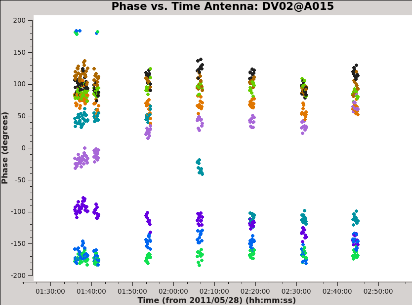
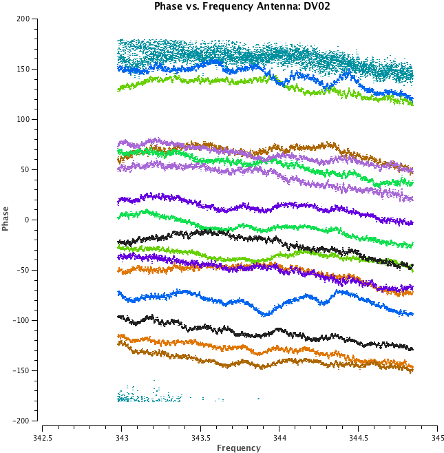
# In CASA
plotms(vis= asdm+'.split.ms',
            xaxis='freq', yaxis='phase',
            selectdata=True, field='3c279', corr='XX', antenna='*&*',
            avgtime='1e8', avgscan=T,
            coloraxis='baseline', iteraxis='antenna')
# In CASA
plotms(vis= asdm+'.split.ms',
           xaxis='time', yaxis='phase',
           selectdata=True, field='3c279', spw='0:40~3800', antenna='*&*',corr='XX',
           avgchannel='3840',  avgscan=T,
           coloraxis='baseline', iteraxis='antenna')
Figure 7 shows that the phase variation as function of time, although smoothly varying, will need to be calibrated in order to obtain proper bandpass solutions. In Figure 8 we see that phase variations in dataset uid_A002_X1ff7b0_Xb are small, typically ~ 30 degrees.
We issue gaincal on 3c279 to determine phase(-only) gain solutions. We will use solint='int' for the solution interval, which means that one gain solution will be determined for every integration time. This short integration time is possible because the bandpass calibrator is a very bright point source, so we have very high signal-to-noise and a perfect model. This will correct for any phase variations in the bandpass calibrator as a function of time, a step which will prevent decorrelation of the vector-averaged bandpass solutions. We will then apply these solutions on-the-fly when we run bandpass.
We will use the average of channels 40~3800 and two spw to increase our signal-to-noise in the determination of the antenna-based phase solutions. Averaging over a subset of channels near the center of the bandpass is acceptable when the phase variation as a function of channel is small. For our reference antenna, we choose DV06. We call the output calibration table asdm+'.g1.cal'. We then check the time variations of the phase solutions with plotcal. We will plot the XX and YY polarization products separately and make different subplots for each of the spectral windows. This is done by setting the "iteration" parameter to "spw" and specifying subplot=221. By setting the parameter "figfile" to a non-blank value, it will also generate png files of the plots.
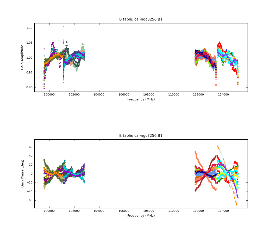
Now that we have a first measurement of the phase variations as a function of time, we can determine the bandpass solutions with bandpass. We will apply the phase calibration table on-the-fly with the parameter "gaintable". Now that the phases are corrected, the data can be time-averaged over longer intervals to maximise SNR in each individual channel. We determine bandpass solutions for both days separately because we find that for some antennas, the response across the bandwidth has changed slightly in between the two sessions. We first calculate the bandpass solution for the first day. Do not worry about the message "Insufficient unflagged antennas", which relates to the flagged edge channels. We then plot the bandpass solutions with plotcal again, and we see that the solutions seem reasonable.
for asdm in basename_all:
  os.system('rm -rf '+asdm+'.g1.cal,'+asdm+'.b1.cal')
  gaincal(vis = asdm+'.split.ms',spw = '0:40~3800,1:40~3800',caltable = asdm+'.g1.cal',field = '3c279',selectdata=T,solint = 'int',refant = 'DV06',calmode='p')
  plotcal(caltable = asdm+'.g1.cal',iteration = 'spw,antenna',subplot = 221,plotrange=[0,0,-180,180],xaxis = 'time',yaxis = 'phase')
  bandpass(vis = asdm+'.split.ms',gaintable = [asdm+'.g1.cal'],caltable = asdm+'.b1.cal',field = '3c279',bandtype='B',solint = 'inf',combine = 'scan', solnorm=T,refant = 'DV06',minblperant=3,minsnr=2,fillgaps=1)
  plotcal(caltable = asdm+'.b1.cal',xaxis = 'freq',yaxis = 'amp',plotrange = [0,0,0.7,1.3],iteration = 'spw',subplot = 211,poln='X',figfile=asdm+'-b1-X-amp_vs_freq.png',showgui=F)
where
- caltable = asdm+'.b1.cal': Output bandpass calibration table
- gaintable = 'asdm+'.g1.cal': Gain calibration table to apply
- minblperant=3: Minimum number of baselines required per antenna for each solve
- minsnr=2: Minimum SNR for solutions
- solint='inf': This setting, combined with the default combine='scan', sets the solution interval to the entire observation
- combine='scan': The solutions cross scans
- bandtype='B': The default type of bandpass solution, which does a channel by channel solution for each specified spw
- fillgaps=1: Interpolate channel gaps 1 channel wide
- solnorm=T: Normalize the bandpass amplitudes and phases of the corrections to unity
Flux Calibration
The first step is to set the flux density for Titan using the task setjy. We will use the Butler-JPL-Horizons 2010 model. We will do a new gain calibration, this time applying the bandpass calibration solutions on-the-fly. We solve for amplitude and phase simultaneously and determine average solutions per scan. Finally, we will bootstrap the flux density of the secondary calibrator from that of Titan using the task fluxscale.
for asdm in basename_all:
  os.system('rm -rf '+asdm+'.g2.cal,'+asdm+'.f1.cal')
  #  Put in Model for Titan
  default('setjy')
  setjy(vis = asdm+'.split.ms',field = 'Titan',standard = 'Butler-JPL-Horizons 2010')
  #2011-05-30 06:48:35 INFO setjy	       Titan  spwid=  1  [I=2.817, Q=0, U=0, V=0] Jy, (JPL-Butler Solar System Object)
  #  Do gaincal in Titan and 3c279
  gaincal(vis = asdm+'.split.ms',gaintable = asdm+'.b1.cal',caltable = asdm+'.g2.cal',refant = 'DV06',solint = 'int',field = 'Titan, 3c279')
  #plotcal(caltable = asdm+'.g2.cal',xaxis = 'time',yaxis = 'amp', iteration = 'antenna',subplot = 421, plotrange = [0,0,0,0],field = 'Titan, 3c279')
  #plotcal(caltable = asdm+'.g2.cal',xaxis = 'time',yaxis = 'phase', iteration = 'antenna',subplot = 421, plotrange=[0,0,-180,180],field = 'Titan, 3c279')
  #  Get flux densities using fluxscale
  fluxscale(vis = asdm+'.split.ms',caltable = asdm+'.g2.cal',fluxtable = asdm+'.f1.cal',reference = 'Titan',transfer = '3c279')
The flux density of Titan is 2.846 Jy at 343 GHz (spw 0) and raises to 3.036 Jy at 353 GHz (spw 1):
  #2011-07-13 07:31:04 INFO setjy	       Titan  spwid=  0  [I=2.846, Q=0, U=0, V=0] Jy, (JPL-Butler Solar System Object)
  #2011-07-13 07:31:13 INFO setjy	       Titan  spwid=  1  [I=3.036, Q=0, U=0, V=0] Jy, (JPL-Butler Solar System Object)
The new flux table asdm+'.f1.cal' replaces the previous asdm+'.g2.cal table in future application of the calibration to the data, i.e. the new flux table contains both asdm+'.g2.cal2 and the newly acquired flux scaling. Unlike the gain calibration steps, this is not an incremental table.
- caltable = 'asdm+'.g2.cal: the output gain calibration table
- minsnr=1.0: To reject solutions with a signal-to-noise less than 1.0
- calmode = 'ap': To solve for amplitude and phase
- solint='inf': Together with the default for the "combine" parameter, this setting will solve for one solution per scan
- solnorm=F: We do not want to normalize the solutions to unity since we wish to relate the measured amplitudes of the secondary calibrator (3c279) to the flux calibrator (Titan)
- gaintable = asdm+'.b1.cal': We apply the bandpass calibration on-the-fly
Now we will examine the amplitude and phase solutions as a function of time, iterating on spectral window and plotting the XX and YY correlations separately for clarity. Zoom in on the GUI to examine the plots in more detail. You can also use the "Mark Region" and "Locate" buttons on the toolbar to identify points. Use the field parameter to select which calibrator you want to plot the solutions for.
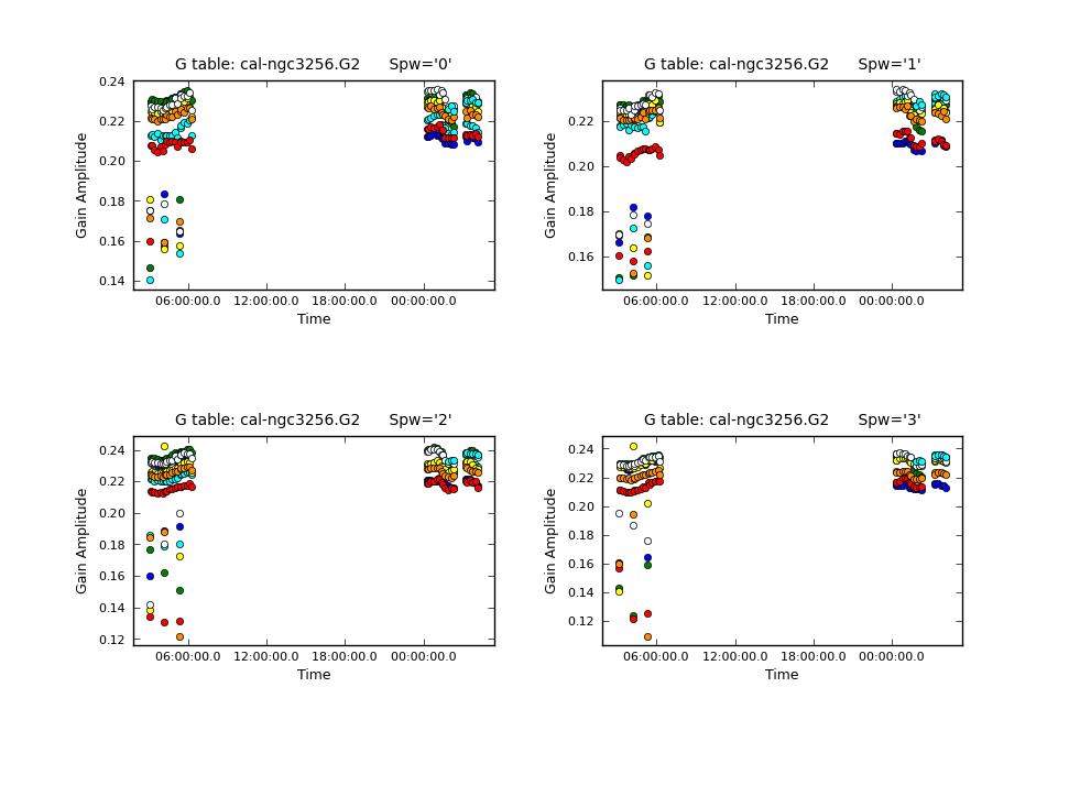
We find that the flux density of 1037-295 is ~10 Jy in the higher frequency spectral windows and ~10.2 Jy in the lower frequency spectral windows. This fluxes agree very well with the 0.8mm measurements from the SMA calibrator [1]: 17 Feb 2011 SMA 8.93 ± 0.82.
Applying the calibrations
Now we will use applycal to apply the bandpass and gaincal tables that we generated in the previous sections. First, we will apply the solutions from the secondary calibrator to the science target and the secondary calibrator itself.
for asdm in basename_all:
  applycal(vis = asdm+'.split.ms', gaintable = [asdm+'.b1.cal',asdm+'.f1.cal'])
Checking the calibration
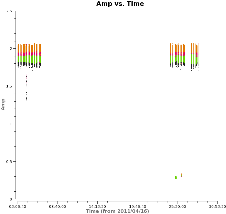
We plot the corrected amplitudes and phases of 3c279 as a function of time and frequency, to check that the phases are close to zero and the amplitudes are constant. The result of the amplitude versus time plot is shown to the right.
# In CASA
asdm=basename_all[0]
plotms(vis = asdm+'.split.ms', xaxis='time', yaxis='amp',
	ydatacolumn='corrected', selectdata=True, field='3c279',
	averagedata=True, avgchannel='3840', avgtime='',
	avgscan=False, avgbaseline=F, coloraxis='spw')

plotms(vis = asdm+'.split.ms', xaxis='time', yaxis='pha',
	ydatacolumn='corrected', selectdata=True, field='3c279',
	averagedata=True, avgchannel='3840', avgtime='',
	avgscan=False, avgbaseline=F, coloraxis='spw')
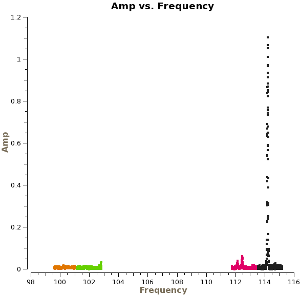
Next we use plotms to examine the corrected amplitude and phase of Antennae as a function of frequency, just by changing the field to field='NGC*','Antennae*'
Split source data and smoothing
We split the spectral window 0 for Antennae galaxies,where CO(3-2) line is. We separate between Northern and Southern mosaic datasets. We smooth the velocity to a width of 23 channels, corresponding to ~10 km/s.
basename_all_North=["uid___A002_X1ff7b0_Xb","uid___A002_X207fe4_X3a","uid___A002_X207fe4_X3b9","uid___A002_X2181fb_X49"]

for asdm in basename_all_North:
    os.system('rm -rf Antennae-'+asdm+'.cal.ms')
    split(vis = asdm+'.split.ms',outputvis = 'Antennae-'+asdm+'.cal.ms',
             field = ['NGC*'],spw='0',width=23)
    listobs(asdm+'.split.ms')

basename_all_South=["uid___A002_X1ff7b0_X1c8","uid___A002_X207fe4_X1f7","uid___A002_X207fe4_X4d7",
                           "uid___A002_X215db8_X18","uid___A002_X215db8_X1d5","uid___A002_X215db8_X392"]

for asdm in basename_all_South:
    os.system('rm -rf Antennae-'+asdm+'.cal.ms')
    split(vis = asdm+'.split.ms',outputvis = 'Antennae-'+asdm+'.cal.ms',
             field = ['Antennae*'],spw='0',width=23)
    listobs(asdm+'.split.ms')
Concatenating datasets for northern and southern mosaics
Once each individual dataset is calibrated, we finally concatenate the data sets corresponding to one either north and south mosaics into one big measurement set. We define an array "comvis" that contains the names of the measurement sets we wish to concatenate, and then we run the task concat.
# In CASA
comvis_South=[]
comvis_North=[]
for asdm in basename_all_South:
	comvis_South.append('Antennae-'+asdm+'.cal.ms')
for asdm in basename_all_North:
	comvis_North.append('Antennae-'+asdm+'.cal.ms')
os.system('rm -rf Antennae_South.cal.ms,Antennae_North.cal.ms')
concat(vis=comvis_South,concatvis='Antennae_South.cal.ms',timesort=T)
concat(vis=comvis_South,concatvis='Antennae_North.cal.ms',timesort=T)
Daniel Espada 12:00 UT, 14 July 2011