NGC3256Band3 for CASA 3.3: Difference between revisions
mNo edit summary |
No edit summary |
||
| Line 1: | Line 1: | ||
==Overview== | ==Overview== | ||
[To be written by Eric] | [To be written by Eric] | ||
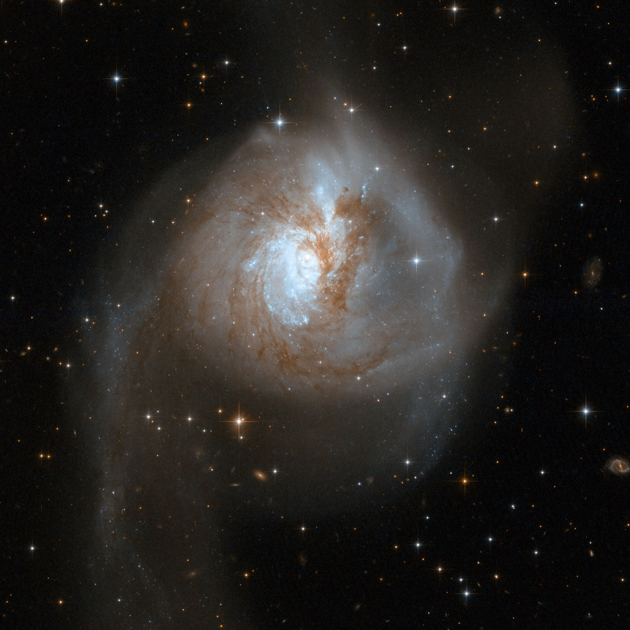
[[File:OpticalImageNGC3256.jpg|200px|thumb|right|HST image of NGC3256]] | |||
==Retrieving the Data== | ==Retrieving the Data== | ||
Revision as of 13:58, 23 May 2011
Overview
[To be written by Eric]
Retrieving the Data
The data were taken in six different datasets over two consecutive nights: April 16-17, 2011. There are three datasets for April 16th and three for April 17th. Here we provide you with "starter" datasets, where we have taken the raw data in ALMA Science Data Model (ASDM) format and converted them to CASA Measurement Sets (MS). We did this using the importasdm task in CASA.
[What else are we going to do to the data we provide?]
Along with the Measurement Sets, we also provide some tables that you will need for the calibration. These include the System Temperature (Tsys) tables, which contain corrections for atmospheric opacity, and Water Vapor Radiometer (WVR) tables, which contain the atmospheric phase corrections determined by the water vapor radiometers on each antenna.
You can download the data here:
[Provide link to the raw .ms files in tar'd, gzip'd format]
Once the download has finished, unpack the file:
# In a terminal outside CASA
tar -xvf ngc3256band3.tgz
[Also provide links to the calibrated data (but maybe not here...maybe better at end of calibration page?)]
Initial Inspection and A priori Flagging
We will eventually concatenate the six datasets used here into one large dataset. However, we will keep them separate for now, as some of the steps to follow require individual datasets (specifically, the application of the Tsys and WVR tables). We therefore start by defining an array "basename" that includes the names of the six files. This will simplify the following steps by allowing us to loop through the files using a simple for-loop in python.
# In CASA
basename=['uid___A002_X1d54a1_X5','uid___A002_X1d54a1_X174','uid___A002_X1d54a1_X2e3',
'uid___A002_X1d5a20_X5','uid___A002_X1d5a20_X174','uid___A002_X1d5a20_X330']
The usual first step is then to get some basic information about the data. We do this using the task listobs, which will output a detailed summary of each dataset supplied.
# In CASA
for name in basename:
        listobs(vis=name+'.ms')
The output will be sent to the CASA logger. You will have to scroll up to see the individual output for each of the six datasets. Here is an example of the most relevant output for the first file in the list.
Fields: 3
  ID   Code Name         RA            Decl           Epoch   SrcId nVis
  0    none 1037-295     10:37:16.0790 -29.34.02.8130 J2000   0     38759
  1    none Titan        00:00:00.0000 +00.00.00.0000 J2000   1     16016
  2    none NGC3256      10:27:51.6000 -43.54.18.0000 J2000   2     151249
  (nVis = Total number of time/baseline visibilities per field)
Spectral Windows:  (9 unique spectral windows and 2 unique polarization setups)
  SpwID  #Chans Frame Ch1(MHz)    ChanWid(kHz)TotBW(kHz)  Ref(MHz)    Corrs
  0           4 TOPO  184550      1500000     7500000     183300      I
  1         128 TOPO  113211.988  15625       2000000     113204.175  XX  YY
  2           1 TOPO  114188.55   1796875     1796875     113204.175  XX  YY
  3         128 TOPO  111450.813  15625       2000000     111443      XX  YY
  4           1 TOPO  112427.375  1796875     1796875     111443      XX  YY
  5         128 TOPO  101506.187  15625       2000000     101514      XX  YY
  6           1 TOPO  100498.375  1796875     1796875     101514      XX  YY
  7         128 TOPO  103050.863  15625       2000000     103058.675  XX  YY
  8           1 TOPO  102043.05   1796875     1796875     103058.675  XX  YY
Sources: 48
  ID   Name         SpwId RestFreq(MHz)  SysVel(km/s)
  0    1037-295     0     -              -
  0    1037-295     9     -              -
  0    1037-295     10    -              -
  0    1037-295     11    -              -
  0    1037-295     12    -              -
  0    1037-295     13    -              -
  0    1037-295     14    -              -
  0    1037-295     15    -              -
  0    1037-295     1     -              -
  0    1037-295     2     -              -
  0    1037-295     3     -              -
  0    1037-295     4     -              -
  0    1037-295     5     -              -
  0    1037-295     6     -              -
  0    1037-295     7     -              -
  0    1037-295     8     -              -
  1    Titan        0     -              -
  1    Titan        9     -              -
  1    Titan        10    -              -
  1    Titan        11    -              -
  1    Titan        12    -              -
  1    Titan        13    -              -
  1    Titan        14    -              -
  1    Titan        15    -              -
  1    Titan        1     -              -
  1    Titan        2     -              -
  1    Titan        3     -              -
  1    Titan        4     -              -
  1    Titan        5     -              -
  1    Titan        6     -              -
  1    Titan        7     -              -
  1    Titan        8     -              -
  2    NGC3256      0     -              -
  2    NGC3256      9     -              -
  2    NGC3256      10    -              -
  2    NGC3256      11    -              -
  2    NGC3256      12    -              -
  2    NGC3256      13    -              -
  2    NGC3256      14    -              -
  2    NGC3256      15    -              -
  2    NGC3256      1     -              -
  2    NGC3256      2     -              -
  2    NGC3256      3     -              -
  2    NGC3256      4     -              -
  2    NGC3256      5     -              -
  2    NGC3256      6     -              -
  2    NGC3256      7     -              -
  2    NGC3256      8     -              -
Antennas: 7:
  ID   Name  Station   Diam.    Long.         Lat.
  0    DV04  J505      12.0 m   -067.45.18.0  -22.53.22.8
  1    DV06  T704      12.0 m   -067.45.16.2  -22.53.22.1
  2    DV07  J510      12.0 m   -067.45.17.8  -22.53.23.5
  3    DV08  T703      12.0 m   -067.45.16.2  -22.53.23.9
  4    DV09  N602      12.0 m   -067.45.17.4  -22.53.22.3
  5    PM02  T701      12.0 m   -067.45.18.8  -22.53.22.2
  6    PM03  J504      12.0 m   -067.45.17.0  -22.53.23.0
This output shows that three fields were observed: 1037-295, Titan, and NGC3256. Field 0 (1037-295) will serve as the gain calibrator and bandpass calibrator; field 1 (Titan) will serve as the flux calibrator; and field 2 (NGC3256) is, of course, the science target.
Note that there are more than four SpwIDs even though the observations were set up to have four spectral windows. The spectral line data themselves are found in spectral windows 1,3,5,7, which have 128 channels each. The first one (spw 1) is centered on the CO(1-0) emission line in the galaxy NGC 3256 and is our highest frequency spectral window. There is one additional spectral window (spw 3) in the Upper Side Band (USB), and there are two spectral windows (spw 5 and 7) in the Lower Side Band (LSB). These additional spectral windows are used to measure the continuum emission in the galaxy, and may contain other emission lines as well.
Spectral windows 2,4,6,8 contain channel averages of the data in spectral windows 1,3,5,7, respectively. These are not useful for the offline data reduction. Spectral window 0 contains the WVR data. You may notice that there are additional SpwIDs listed in the "Sources" section which are not listed in the "Spectral Windows" section. These spectral windows are reserved for the WVRs of each antenna (seven in our case). At the moment, all WVRs point to spw 0, which contains nominal frequencies. The additional spectral windows (spw 9-15) are therefore not used and can be ignored.
Another important thing to note is that the position of Titan is listed as 00:00:00.0000 +00.00.00.0000. This is due to the fact that for ephemeris objects, the positions are currently not stored in the asdm. This will be handled correctly in the near future, but at present, we have to fix this offline. We will correct the coordinates below by running the procedure fixplanet.
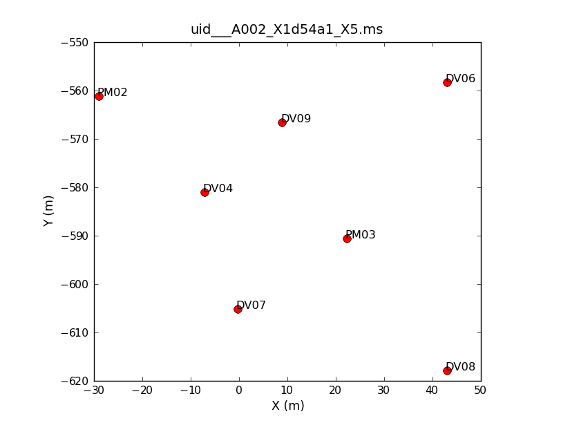
Seven antennas we used for the dataset listed above. Note that numbering in python always begins with "0", so the antennas have IDs 0-6. To see what the antenna configuration looked like at the time of the this observation, we will use the task plotants.
# In CASA
plotants(vis=basename[0]+'.ms', figfile=basename[0]+'_plotants.png')
This will plot the antenna configuration on your screen as well as save it under the specified filename for future reference. This will be important later on when we need to choose a reference antenna, since the reference antenna should be close to the center of the array (as well as stable and present for the entire observation).
If you repeat the plotants command for the other five datasets, you will see that there is an additional antenna (DV10) present on the second day of observations. Other than that, the configuration stays constant during the course of the observations.
Flagging
The first editing we will do is some a priori flagging with flagdata and flagautocorr. We will start by flagging the shadowed data and the autocorrelation data:
# In CASA
for name in basename:
	flagdata(vis=name+'.ms', flagbackup = F, mode = 'shadow')
	flagautocorr(vis=name+'.ms')
There are a number of scans in the data that were used by the online system for pointing calibration. These scans are no longer needed, and we can flag them easily with flagdata by selecting on 'intent':
# In CASA
for name in basename:
        flagdata(vis=name+'.ms', mode='manualflag', flagbackup = F, intent='*POINTING*')
Similarly, we can flag the scans corresponding to atmospheric calibration:
# In CASA
for name in basename:
        flagdata(vis=name+'.ms', mode='manualflag', flagbackup = F, intent='*ATMOSPHERE*')
We will then store the current flagging state for each dataset using the flagmanager:
# In CASA
for name in basename:
        flagmanager(vis = name+'.ms', mode = 'save', versionname = 'Apriori')
We will continue with some initial flagging/corrections specific to these datasets. For uid___A002_X1d54a1_X174.ms there is a outlying feature in spw=7, antenna DV04. This corresponds to scans 5 and 9, so we flag those data:
# In CASA
flagdata(vis='uid___A002_X1d54a1_X174.ms', mode='manualflag',
	antenna='DV04', flagbackup = F, scan='5,9', spw='7')
Antenna DV07 shows large delays for the first three datasets. We correct this by calculating a K-type delay calibration table with gencal. The parameters are the delays measured in nanoseconds, first cycling over polarization product, and then over spectral window (thus giving eight numbers in total). Before creating these tables, make sure to delete any existing versions.
# In CASA
for i in range(3): # loop over the first three ms's
	name=basename[i]
	os.system('rm -rf '+name+'_del.K')
	gencal(vis=name+'.ms', caltable=name+'_del.K',
	caltype='sbd', antenna='DV07', pol='X,Y', spw='1,3,5,7',
        parameter=[0.99, 1.10, -3.0, -3.0, -3.05, -3.05, -3.05, -3.05])
The delay values were simply estimated by eye. The purpose here is to get the phases approximately flat as a function of frequency. Any additional phase variations will be corrected for later when we do the bandpass calibration.
Note that when you run the gencal command above, CASA may generate the warning "No scr col generation!!!" This just means that there is no field association in the tables generated, so that you can apply them to any of the fields in the observation. This is not important, so you can ignore the warning.
We will apply these K tables to the data in the next section.
WVR Correction and Tsys Calibration
We will now apply the delay correction table and the WVR calibration tables to the data with the task applycal. We do this in two steps. First we will cycle over the three datasets from the first day of observations, because we have to correct the delay error for DV07 for those data. For the last three datasets (i.e. those taken during the second day), we do not need to correct the delays, so we just apply the WVR tables. In the call to applycal, we will specify interpolation="nearest". This is important for the WVR corrections, and it doesn't make a difference for the delay corrections because they have no time dependence.
# In CASA
for i in range(3): # loop over the first three data sets
	name=basename[i]
	applycal(vis=name+'.ms', flagbackup=F, spw='1,3,5,7',
		 interp=['nearest','nearest'], gaintable=[name+'_del.K',name+'.W'])

for i in range(3,6): # loop over the last three data sets
	name=basename[i]
	applycal(vis=name+'.ms', flagbackup=F, spw='1,3,5,7',
		 interp='nearest', gaintable=name+'.W')
Now we split out the corrected_data column of the datasets with the task split. We give the resulting datasets the extension "_K_WVR" to indicate that the delay tables and WVR tables have been applied in the data column, and we specify spectral windows 0-8 to get rid of the "WVR placeholder" spectral windows. Again, we are careful to remove any previous versions of the split ms's before running the split command.
# In CASA
for name in basename:
	os.system('rm -rf '+name+'_K_WVR.ms*')
	split(vis=name+'.ms', outputvis=name+'_K_WVR.ms',
		datacolumn='corrected', spw='0~8')
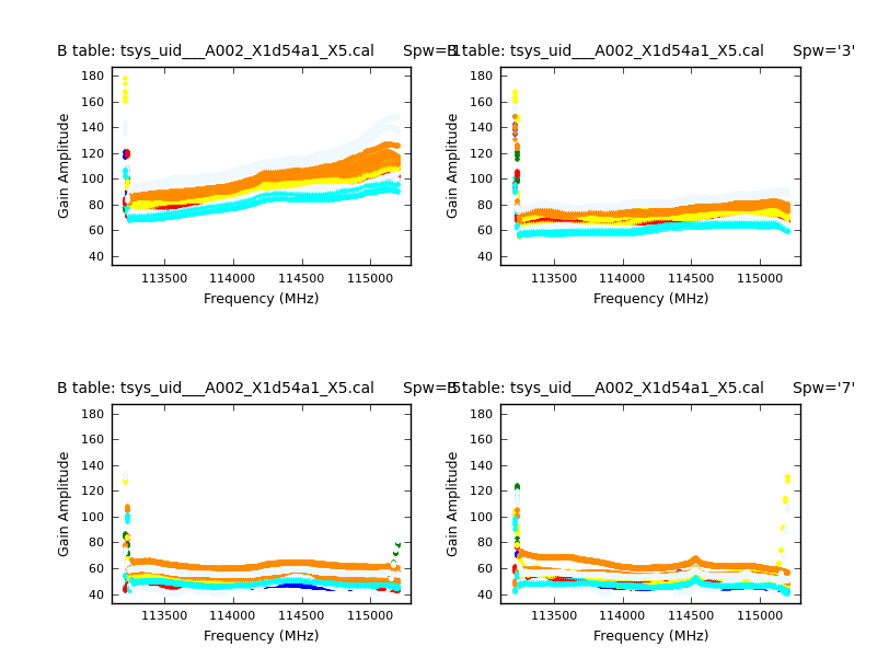
Next we do the Tsys calibration. Tsys measurements correct for the atmospheric opacity (to first-order) and allow the calibration sources to be measured at elevations that differ from the science target. The Tsys tables for these datasets were provided with the downloadable data. We will start by inspecting them with the task plotcal:
# In CASA
for name in basename:
	plotcal(caltable='tsys_'+name+'.cal', xaxis='freq', yaxis='amp',
                spw='1,3,5,7', subplot=221, overplot=False,
                iteration='spw', plotrange=[0, 0, 40, 180], plotsymbol='.',
                figfile='tsys_per_spw'+name+'.png')
Note that we only plot the spectral windows with the spectral line data. In addition to plotting on your screen, the above command will also produce a plot file (png) for each of the six datasets. An example plot is shown to the right for the first dataset.
Aside from the large amplitudes in the edge channels (which we will handle below), the plots look acceptable. Note that in the lowest frequency spectral window, Tsys rises toward higher frequencies. This is because we are observing right at the edge of Band 3.
We will apply the Tsys tables with applycal: We do this for each field separately so that the appropriate calibration data are applied to the right fields. The "field" parameter specifies the field to which we will apply the calibration, and the "gainfield" parameter specifies the field from which you wish to take the calibration solutions from the gaintable.
# In CASA
for name in basename:
	for field in ['Titan','1037*','NGC*']:
		applycal(vis=name+'_K_WVR.ms', spw='1,3,5,7', flagbackup=F, field=field, gainfield=field,
			interp='nearest', gaintable=['tsys_'+name+'.cal'])
We then once again split out the corrected_data column, this time only retaining spectral windows 1,3,5,7. This will get rid of the extraneous spectral windows, including the channel averaged spectral windows and spw 0, which is the one for the WVR data.
# In CASA
for name in basename:
	os.system('rm -rf '+name+'_line.ms*')
	split(vis=name+'_K_WVR.ms', outputvis=name+'_line.ms',
		datacolumn='corrected', spw='1,3,5,7')
The WVR and Tsys tables are now applied in the data column of the new measurement sets. These datasets have the extension "_line" to indicate that they only contain the spectral line data and no longer the "channel average" spectral windows. These measurement sets therefore have four spectral windows, with IDs 0-3.
Now that we have applied the Tsys calibration and WVR corrections, we can concatenate the six individual data sets into one big measurement set. We define an array "comvis" that contains the names of the measurement sets we wish to concatenate, and then we run the task concat.
# In CASA
comvis=[]
for name in basename:
	comvis.append(name+'_line.ms')

os.system('rm -rf ngc3256_line.ms*')
concat(vis=comvis, concatvis='ngc3256_line.ms')
Additional Data Inspection
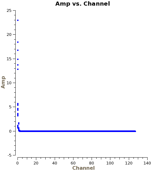
Now that the data are concatenated into one dataset, we will do some additional inspection with plotms. First we will plot amplitude versus channel, averaging over time and baselines in order to speed up the plotting process.
# In CASA
plotms(vis='ngc3256_line.ms', xaxis='channel', yaxis='amp',
       averagedata=T, avgbaseline=T, avgtime='1e8', avgscan=T)
From this plot we see that the edge channels have abnormally high amplitudes. We will use flagdata to remove the edge channels from both sides of the bandpass:
# In CASA
flagdata(vis = 'ngc3256_line.ms', flagbackup = F, spw = ['*:0~10','*:125~127'])
Next, we will look at amplitude versus time, averaging over all channels and colorizing by field. Since the observations take place over two days, you will need to zoom in to examine the data in more detail. In particular, note the difference in Titan's amplitude between the two days and the change in amplitude during the second day. The plot on the right shows a zoom-in on the first day of observations. Scans on Titan are colored red, NGC3256 is orange, and the calibrator 1037-295 is colored black.
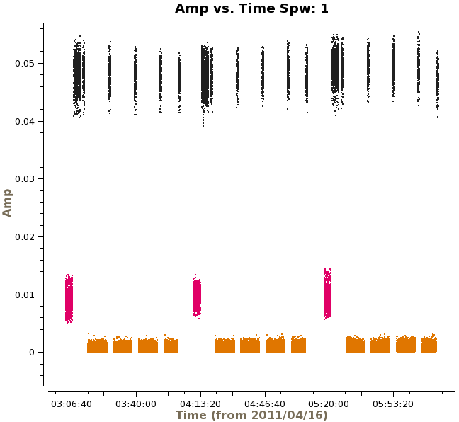
# In CASA
plotms(vis='ngc3256_line.ms', xaxis='time', yaxis='amp',
       averagedata=T, avgchannel='128', coloraxis='field')
Titan is our primary flux calibrator. However, for the second day of observations, Titan had moved to close to Saturn, and Saturn's rings moved into the primary beam. Another way to see this is to plot amplitude versus uv-distance and colorize by scan:
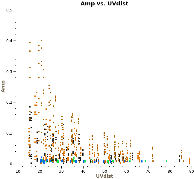
# In CASA
plotms(vis='ngc3256_line.ms', xaxis='uvdist', yaxis='amp', field='1',
       averagedata=T, avgchannel='128', avgtime='1e8', coloraxis='scan')
If you use the "Mark a region" and "Locate" tools in plotms, you will see the signature of a bright, resolved source during the latter three (last day's) scans. We will therefore need to flag the Titan scans for the second day:
# In CASA
flagdata(vis = 'ngc3256_line.ms', flagbackup = F,
	timerange='>2011/04/16/12:00:00', field='Titan')
Next, we will fix the position of Titan in the combined dataset. Recall that the position of the Titan field is currently set to 00:00:00.0000 +00.00.00.0000. The following procedure will replace this with the actual position observed by the telescopes and, at the same time, it will recalculate the uvw coordinates:
# In CASA
execfile(os.getenv("CASAPATH").split(' ')[0]+"/lib/python2.6/recipes/fixplanets.py") # linux
#execfile(os.getenv("CASAPATH").split(' ')[0]+"/Resources/python/recipes/fixplanets.py") # Mac
fixplanets('ngc3256_line.ms', 'Titan', True)
Note that on a Mac, the path to fixplanets.py is different than on Linux machines. The third parameter in fixplanets, set to True, indicates that the uvw-coordinates for Titan are recalculated. Note that for Cycle 0 data, the coordinates of ephemeris objects will be treated correctly in the data.
Continue to inspect the data with plotms, plotting different axes and colorizing by the different parameters. Don't forget to average the data if possible to speed the plotting process. You will find the following:
- Baselines with DV07 have very high amplitudes in spw 3, correlation YY
- Baselines with DV08 have very low amplitudes in spw 3, correlation YY, but only for the last observation
- Baselines with PM03 have low amplitudes at 2011/04/17/02:15:00 for spw 0
- Baselines with PM03 have low amplitudes at 2011/04/16/04:15:15 for spw 2 and 3
We flag the bad data with the following commands:
# In CASA
flagdata(vis='ngc3256_line.ms', flagbackup=F, spw='3',
	 correlation='YY', mode='manualflag', selectdata=T,
	 antenna='DV07', timerange='')

flagdata(vis='ngc3256_line.ms', flagbackup=F, spw='3',
	 correlation='YY', mode='manualflag', selectdata=T,
	 antenna='DV08', timerange='>2011/04/17/03:00:00')

flagdata(vis='ngc3256_line.ms', flagbackup=F, spw='0',
	 mode='manualflag', selectdata=T, antenna='PM03',
	 timerange='2011/04/17/02:15:00~02:15:50')

flagdata(vis='ngc3256_line.ms', flagbackup=F, spw='2,3',
	 mode='manualflag', selectdata=T, antenna='PM03',
	 timerange='2011/04/16/04:13:50~04:18:00')
Bandpass Calibration
We are now ready to begin the bandpass calibration. First, we will inspect the bandpass calibrator by plotting the phase as a function of frequency and time. For the first plot we use avgscan=T and avgtime='1E6' to average in time over all scans, and we specify coloraxis='baseline' to colorize by baseline. For the second, we use spw='0:30~90' and avgchannel='128' to average over the central 61 channels of the first spectral window.
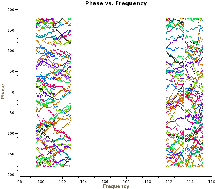
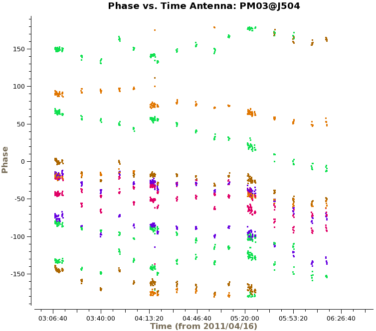
# In CASA
plotms(vis='ngc3256_line.ms', xaxis='freq', yaxis='phase', selectdata=True,
	field='1037*', avgtime='1E6', avgscan=T, coloraxis='baseline', iteraxis='antenna')

plotms(vis='ngc3256_line.ms', xaxis='time', yaxis='phase', selectdata=True,
	field='1037*', spw='0:30~90', avgchannel='128', avgscan=T,
        coloraxis='baseline', iteraxis='antenna')
The plot on the right shows the time-averaged phase as a function of frequency for the calibrator 1037-295, for all baselines. We see that the phase variations across the spectral windows are modest, typically ~30 degrees. The second plot shows how the phase varies as function of time. For clarity, we only show baselines with one antenna and only for the first day of observations. There are clearly phase variations on short time scales, that we wish to correct for before calculating the bandpass solutions.
Hence, we run gaincal on the bandpass calibrator to determine phase-only gain solutions. We will use solint='int' for the solution interval, which means that one gain solution will be determined for every integration time. This will correct for any phase variations in the bandpass calibrator as a function of time, a step which will prevent decorrelation of the vector-averaged bandpass solutions. We will then apply these solutions on-the-fly when we run bandpass.
We will use the average of channels 40 to 80 to increase our signal-to-noise in the determination of the antenna-based phase solutions. Averaging over a subset of channels near the center of the bandpass is acceptable when the phase variation as a function of channel is small, which it is here. For our reference antenna, we choose PM03. We call the output calibration table "ngc3256.G1".
# In CASA
gaincal(vis = 'ngc3256_line.ms', caltable = 'ngc3256.G1', spw = '*:40~80', field = '1037*',
        selectdata=T, solint= 'int', refant = 'PM03', calmode = 'p')
We then check the time variations of the phase solutions with plotcal. We will plot the XX and YY polarization products separately and make different subplots for each of the spectral windows. This is done by setting the "iteration" parameter to "spw" and specifying subplot=221. By setting the parameter "figfile" to a non-blank value, it will also generate png files of the plots.
# In CASA
plotcal(caltable = 'ngc3256.G1', xaxis = 'time', yaxis = 'phase',
	poln='X', plotsymbol='o', plotrange = [0,0,-180,180], iteration = 'spw',
	figfile='phase_vs_time_XX.G1.png', subplot = 221)

plotcal(caltable = 'ngc3256.G1', xaxis = 'time', yaxis = 'phase',
	poln='Y', plotsymbol='o', plotrange = [0,0,-180,180], iteration = 'spw',
	figfile='phase_vs_time_YY.G1.png', subplot = 221)
Now that we have a first measurement of the phase variations as a function of time, we can determine the bandpass solutions with bandpass. We will apply the phase calibration table on-the-fly with the parameter "gaintable".
# In CASA
bandpass(vis = 'ngc3256_line.ms', caltable = 'ngc3256.B1', gaintable = 'ngc3256.G1',
	field = '1037*', minblperant=3, minsnr=2, solint='inf',
	bandtype='B', fillgaps=1, refant = 'PM03', solnorm = T)
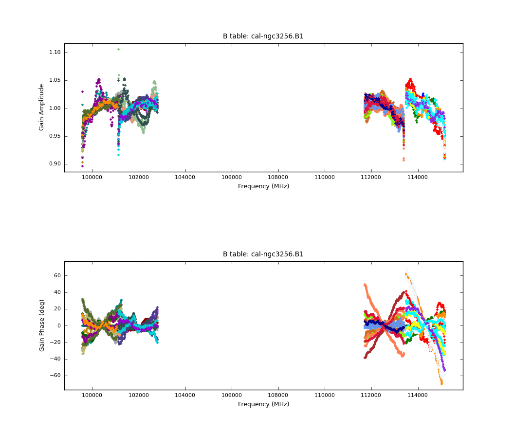
- caltable = 'ngc3256.B1': output bandpass calibration table
- gaintable = 'ngc3256.G1': gain calibration table to apply
- minblperant=3: Minimum number of baselines required per antenna for each solve
- minsnr=1: Minimum SNR for solutions
- solint='inf': This setting, combined with the default combine='scan', sets the solution interval to the entire observation
- bandtype='B': The default type of bandpass solution, which does a channel by channel solution for each specified spw
- fillgaps=1: Interpolate channel gaps 1 channel wide
- solnorm=T: Normalize the bandpass amplitudes and phases of the corrections to unity
We then plot the bandpass solutions with the following commands:
# In CASA
plotcal(caltable = 'ngc3256.B1', xaxis='freq', yaxis='phase', spw='',
	subplot=212, overplot=False, plotrange = [0,0,-70,70],
	plotsymbol='.', timerange='')

plotcal(caltable = 'ngc3256.B1', xaxis='freq', yaxis='amp', spw='',
	subplot=211, overplot=False,
	figfile='bandpass.B1.png', plotsymbol='.', timerange='')
[PERHAPS APPLY THE SOLUTIONS AND SHOW PLOTS HERE?]
Gain Calibration
The first step is to set the flux density for Titan using the task setjy. We will use the Butler-JPL-Horizons 2010 model:
# In CASA
setjy(vis='ngc3256_line.ms', field='Titan', standard='Butler-JPL-Horizons 2010')
The flux density of Titan is 297 mJy at 103 GHz (spw 3):
2011-05-22 09:42:58 INFO setjy Titan spwid= 3 [I=0.2966, Q=0, U=0, V=0] Jy, (JPL-Butler Solar System Object)
Now we will do a new gain calibration, this time applying the bandpass calibration solutions on-the-fly. We solve for amplitude and phase simultaneously and determine average solutions per scan:
# In CASA
gaincal(vis = 'ngc3256_line.ms', caltable = 'ngc3256.G2', spw =
	'*:16~112', field = '1037*,Titan', minsnr=1.0,
	solint= 'inf', selectdata=T, solnorm=False, refant = 'DV04',
	gaintable = 'ngc3256.B1', calmode = 'ap')
- caltable = 'ngc3256.G2': the output gain calibration table
- minsnr=1.0: To reject solutions with a signal-to-noise less than 1.0
- calmode = 'ap': To solve for amplitude and phase
- spw='*:16~112': to select all spectral windows, but only the inner 75% of the channels of each
- solint='inf': Together with the default for the "combine" parameter, this setting will solve for one solution per scan
- solnorm=F: We do not want to normalize the solutions to unity since we wish to relate the measured amplitudes of the secondary calibrator (1037-295) to the flux calibrator (Titan)
- gaintable = ['ngc3256.B1']: We apply the bandpass calibration on-the-fly
[ANOTHER QUESTION: WHY DO YOU RESTRICT THE CHANNEL RANGE ABOVE? - To avoid the edge effects. I now changed to the inner 75% of channels]
Now we will examine the amplitude and phase solutions as a function of time, iterating on spectral window and plotting the XX and YY correlations separately for clarity. Zoom in on the GUI to examine the plots in more detail. You can also use the "Mark Region" and "Locate" buttons on the toolbar to identify points. Use the field parameter to select which calibrator you want to plot the solutions for.
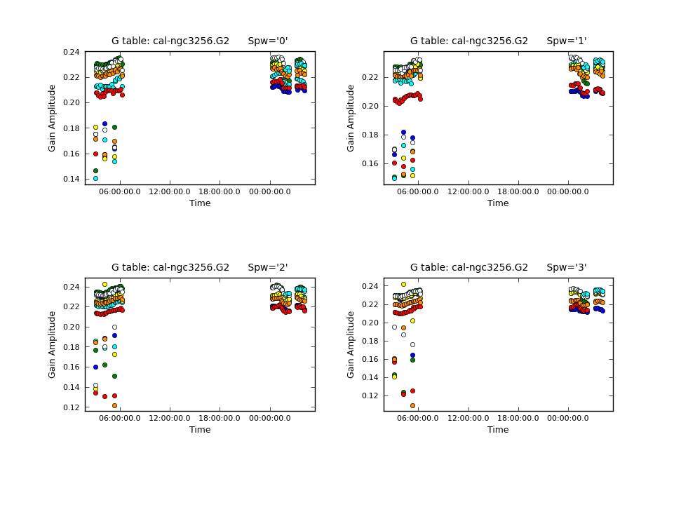
# In CASA
plotcal(caltable = 'ngc3256.G2', xaxis = 'time', yaxis = 'phase',
	poln='X', plotsymbol='o', plotrange = [0,0,-180,180], iteration= 'spw',
        figfile='phase_vs_time_XX.G2.png', subplot = 221)

plotcal(caltable = 'ngc3256.G2', xaxis = 'time', yaxis = 'phase',
	poln='Y', plotsymbol='o', plotrange = [0,0,-180,180], iteration= 'spw',
        figfile='phase_vs_time_YY.G2.png', subplot = 221)

plotcal(caltable = 'ngc3256.G2', xaxis = 'time', yaxis = 'amp',
	poln='X', plotsymbol='o', plotrange = [], iteration = 'spw',
	figfile='amp_vs_time_XX.G2.png', subplot = 221)

plotcal(caltable = 'ngc3256.G2', xaxis = 'time', yaxis = 'amp',
	poln='Y', plotsymbol='o', plotrange = [], iteration = 'spw',
	figfile='amp_vs_time_YY.G2.png', subplot = 221)
We find very stable amplitude solutions for the phase calibrator. The lower points for the first day, are the solutions for Titan.
Finally, we will bootstrap the flux density of the secondary calibrator from that of Titan using the task fluxscale. The new flux table ngc3256.G2.flux replaces the previous ngc3256.G2 table in future application of the calibration to the data, i.e. the new flux table contains both ngc3256.G2 and the newly acquired flux scaling. Unlike the gain calibration steps, this is not an incremental table.
[WE HAVE TO SAY SOMETHING ABOUT TITAN IN SPW 2 AND 3 HERE...]
# In CASA
fluxscale( vis="ngc3256_line.ms", caltable="ngc3256.G2",
        fluxtable="ngc3256.G2.flux", reference="Titan",
        transfer="1037*", refspwmap=[0,1,1,1])
Note that we previously flagged the Titan scans from the second day due to contamination from nearby Saturn's rings. We have therefore used the Titan scans from the first day alone to flux calibrate both days' observations. This would not always be an acceptable solution; however, in this case, examination of the measured amplitudes for the phase calibrator over both days indicate that the flux scale is relatively stable. The logger produces the following output:
2011-05-23 13:44:19 INFO fluxscale	 Flux density for 1037-295 in SpW=0 is: 1.81706 +/- 0.017641 (SNR = 103.003, nAnt= 7)
2011-05-23 13:44:19 INFO fluxscale	 Flux density for 1037-295 in SpW=1 is: 1.82168 +/- 0.0146764 (SNR = 124.124, nAnt= 7)
2011-05-23 13:44:19 INFO fluxscale	 Flux density for 1037-295 in SpW=2 (ref SpW=1) is: 1.90965 +/- 0.0153382 (SNR = 124.503, nAnt= 7)
2011-05-23 13:44:19 INFO fluxscale	 Flux density for 1037-295 in SpW=3 (ref SpW=1) is: 1.87056 +/- 0.015111 (SNR = 123.788, nAnt= 6)
We find that the flux density of 1037-295 is ~1.8 Jy in all four spectral windows, which agrees very well with the 3mm measurements from the ATCA and OVRO of a few years ago (see SMA calibrator list).
Applying the calibrations
Now we will use applycal to apply the bandpass and gaincal tables that we generated in the previous sections. First, we will apply the solutions from the secondary calibrator to the science target and the secondary calibrator itself. We want to use the solutions from the secondary calibrator for the science target because, as the phase calibrator, it was observed throughout the observations. Its flux scale has also now been bootstrapped to that of the flux calibrator, so it can serve as an amplitude and phase calibrator. The application of the solutions to the secondary calibrator itself is a way for us to check the quality of the calibration. Below, we will do the same for the flux calibrator (Titan), applying its amplitude and phase solutions to itself to check the calibration.
# In CASA
applycal( vis='ngc3256_line.ms', flagbackup=F, field='NGC*,1037*',
	interp=['nearest','nearest'], gainfield = ['1037*', '1037*'],
	gaintable=['ngc3256.G2.flux','ngc3256.B1'])
- gaintable=['ngc3256.G2.flux','ngc3256.B1']: We apply the gaincal table with the correct flux scaling and the bandpass table
- gainfield = ['1037*', '1037*']: We use the solutions from the secondary calibrator (1037-295) in both tables
- interp='nearest': We opt for interpolation mode "nearest"
- flagbackup=F: We do not back up the state of the flags before applying calibration
Let's now use plotms to examine the corrected amplitude of NGC3256 as a function of frequency:
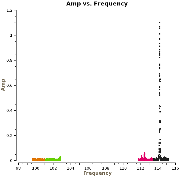
# In CASA
plotms(vis='ngc3256_line.ms', xaxis='freq', yaxis='amp',
	ydatacolumn='corrected', selectdata=True, field='NGC*',
	averagedata=True, avgchannel='', avgtime='10000s',
	avgscan=True, avgbaseline=T, coloraxis='spw')
Use the "Zoom" tool to zoom in on the different spectral windows. (Note that spw 2-3 are on the left). There are three emission lines in spectral windows 0-1. There is no emission in spw 2 and 3. [LOOKS LIKE THERE ARE STILL SOME BAD CHANNELS ON THE EDGE OF SPW 2-3. - that's right. We could flag a few more channels - OK I MAY CHANGE THIS ABOVE THEN. I THINK I DID ~15 BEFORE]
There are some additional bad data points, which we will flag with flagdata. [DID YOU FIND THESE POINTS USING THE ABOVE PLOT? I THINK IT WOULD BE GOOD TO FLAG THINGS AFTER THE PLOT WHERE YOU DISCOVER THEM]
# In CASA
flagdata(vis='ngc3256_line.ms', mode='manualflag',
	timerange='2011/04/16/04:13:35~04:13:45', flagbackup = F)
tget(flagdata)
timerange='2011/04/16/05:21:13~05:21:19'
flagdata()
timerange='2011/04/16/04:16:40~04:16:49'
flagdata()
Note that in the above command sequence, we utilize the CASA function tget. This function retrieves the last input values for the function specified.
At this point, we will image the secondary calibrator as a check of our calibration. We do this using the task clean, after first removing any previous versions of the images that may exist in our directory.
# In CASA
os.system('rm -rf phasecal_cont*')
clean(vis="ngc3256_line.ms", imagename="phasecal_cont", field="1037*",
	spw='*:20~120', selectdata=T, mode="mfs", niter=1000,
	gain=0.1, threshold="0.7mJy", psfmode="clark",
	interactive=False, mask=[126, 126, 130,130], imsize=256,
	cell="1arcsec", weighting="briggs", robust=0.0)
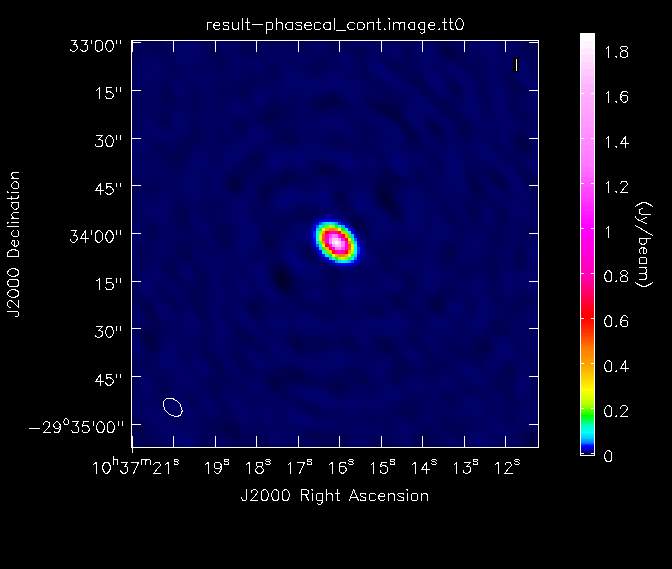
- imagename='phasecal_cont': the base name of the output images
- spw='*:20~120': We image all spectral windows, ignoring the outermost channels of each
- mode='mfs': The default mode, which produces one image from all the specified data combined
- niter=1000: Maximum number of clean iterations
- theshold="0.7mJy": Stop cleaning if the maximum residual is below this value
- mask=[126, 126, 130,130]: Limits the clean component placement to the region of the source
- imsize=256, cell='1arcsec': Chosen to appropriately sample the resolution element and cover the primary beam
- weighting='briggs', robust=0: a weighting scheme that offers a good compromise between sensitivity and resolution
Once the imaging of the secondary calibrator is complete, we will generate some statistics on the image using the task imstat:
# In CASA
calstat=imstat(imagename='phasecal_cont.image', region='', box='160,50,210,210')
rms=(calstat['rms'][0])
print '>> rms in phase calibrator image: '+str(rms)
calstat=imstat(imagename='phasecal_cont.image', region='')
peak=(calstat['max'][0])
print '>> Peak in phase calibrator image: '+str(peak)
print '>> Dynamic range in phase calibrator image: '+str(peak/rms)
Here, we have used the "box" parameter in the first call of imstat to find the image rms in a region away from the strong central point source. The image dynamic range in the calibrator image is ~2500. We will then look at the image of the secondary calibrator with imview.
# In CASA
imview(raster={'file': 'phasecal_cont.image', 'colorwedge':T,
        'range':[-0.004, 0.250], 'scaling':-2.5, 'colormap':'Rainbow 2'},
        out='phasecal_map.png', zoom=1)
This command rasters the image of the phase calibrator to the GUI and outputs the file phasecal_map.png. It uses the Rainbow 2 colomap scheme and includes a colorwedge on the plot. The "range" and "scaling" parameters have been chosen to bring out the weaker features in the map. Overall, the calibration looks pretty good, so we will move on. If the image quality was not acceptable, we would need to flag some more data and redo the calibration to this point.
Now we will apply the calibration to the flux calibrator, Titan, using the solutions we derived for Titan itself.
# In CASA
applycal(vis='ngc3256_line.ms', flagbackup=F, field='Titan',
	interp=['nearest','nearest'], gainfield = ['Titan', '1037*'],
	gaintable=['ngc3256.G2.flux','ngc3256.B1'])
Now we will image the flux calibrator (Titan). See the previous call to clean for a description of the various inputs.
# In CASA
os.system('rm -rf ampcal_cont*')
clean(vis="ngc3256_line.ms", imagename="ampcal_cont",
        field="Titan", spw="0:20~120,1:20~120", mode="mfs", niter=200,
	mask=[126, 126, 130,130], imsize=256,
	cell="1arcsec", weighting="briggs", robust=0.0)
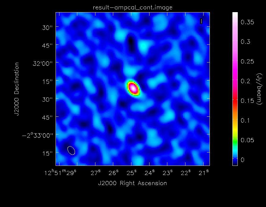
As before, we will generate some statistics on the image:
# In CASA
calstat=imstat(imagename="ampcal_cont.image",region="",box="160,50,210,210")
rms=(calstat['rms'][0])
print ">> rms in amp calibrator image: "+str(rms)
calstat=imstat(imagename="ampcal_cont.image",region="")
peak=(calstat['max'][0])
print ">> Peak in amp calibrator image: "+str(peak)
print ">> Dynamic range in amp calibrator image: "+str(peak/rms)
The dynamic range in this image is ~66. It's much less than the image of the secondary calibrator because less time was spent observing it (the total on-source time on Titan is only 9 minutes). We will then take a look at the image with imview, again choosing the data range and scaling parameter to bring out weak features in the map:
# In CASA
imview(raster={'file': 'ampcal_cont.image', 'colorwedge':T,
        'range':[-0.02, 0.250], 'scaling':-1.5, 'colormap':'Rainbow 2'},
        out='ampcal_map.png', zoom=1)
We are now happy with the images of the calibrators and move on to making images of the galaxy.
Continuum image of the galaxy
Now that we have a fully calibrated data set, we do no longer need the calibrator data and hence we create a new measurement set that only contains the science target NGC 3256. We run split with field='NGC*' to create ngc3256_line_target.ms:
# In CASA
os.system('rm -rf ngc3256_line_target.ms*')
split(vis='ngc3256_line.ms', outputvis='ngc3256_line_target.ms',
	field='NGC*')
We make a continuum image of the galaxy using clean. Most parameters are equal to our previous clean runs, but this time we are careful to select only the channels that are free from CO and CN line emission. We select a mask that just includes the extent of the continuum emission. Here, we use the default non-interactive mode, but if you want to define the clean boxes more carefully, specify interactive=True. In that case, the clean task will bring up a viewer where the clean region can be defined, either by selecting boxes or by selecting polygon regions.
# In CASA
os.system('rm -rf ngc3256.cont*')
clean( vis='ngc3256_line_target.ms', imagename='ngc3256_cont',
	spw='0:20~53;71~120,1:70~120,2:20~120,3:20~120',
	mode='mfs', niter=500, mask=[118,119,147,138],
	imsize=256, cell='1arcsec', weighting='briggs', robust=0.0)
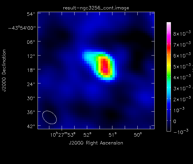
Again, we determine some statistics of the image:
# In CASA
calstat=imstat(imagename='ngc3256_cont.image', region='', box='160,50,210,210')
rms=(calstat['rms'][0])
print '>> rms in continuum image: '+str(rms)
calstat=imstat(imagename='ngc3256_cont.image', region='')
peak=(calstat['max'][0])
print '>> Peak in continuum image: '+str(peak)
print '>> Dynamic range in continuum image: '+str(peak/rms)
This tells us that the peak flux density of the image is ~7 mJy and the dynamic range is approximately 34. For future reference, we create a png file of the continuum image:
# In CASA
imview(raster={'file': 'ngc3256_cont.image', 'colorwedge':T,
        'range':[-0.0003, 0.005], 'scaling':-1, 'colormap':'Rainbow 2'},
        out='ngc3256_cont.png', zoom=2)
The continuum flux is fairly low in this galaxy, but given the large bandwidth of ALMA, we have sufficient signal-to-noise to attempt to self-calibrate the data. We will therefore do some phase-only self-calibration of the image. We do this by deriving gain corrections with gaincal, which will compare the data column with the model column, which has been filled with the clean components from the recent run of clean. We use a solution interval of 15 minutes as we found that this gives just sufficient signal to noise per antenna.
# In CASA
gaincal(vis='ngc3256_line_target.ms', field='NGC*',
    	caltable='ngc3256_cont_900.Gp',
    	spw='0:20~53;71~120,1:70~120,2:20~120,3:20~120',
    	solint='900s', refant='DV04', calmode='p',
    	minblperant=3)
- caltable='ngc3256_cont_900.Gp': The name of the output calibration table
- spw='0:20~53;71~120,1:70~120,2:20~120,3:20~120': To select only the continuum channels
- solint='900s': To specify a 15-minute solution interval
- refant='DV04': Our reference antenna
- calmode='p': To select phase-only solutions
- minblperant=3: To set the minimum number of baselines to other antennas that must be present for a given antenna to have a solution
We then examine the derived phase solutions using plotcal:
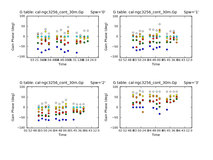
# In CASA
plotcal(caltable = 'ngc3256_cont_900.Gp', xaxis = 'time', yaxis =
	'phase', poln='X', plotsymbol='o', plotrange = [0,0,-180,180],
	iteration = 'spw', figfile='phase_vs_time_XX_900_Gp.png',
	subplot = 221)

plotcal(caltable = 'ngc3256_cont_900.Gp', xaxis = 'time', yaxis =
	'phase', poln='Y', plotsymbol='o', plotrange = [0,0,-180,180],
	iteration = 'spw', figfile='phase_vs_time_YY_900_Gp.png',
	subplot = 221)
The phase-only self-cal solutions look good, so we will apply them to the data with applycal. This will overwrite the data in the corrected_data column.
# In CASA
applycal(vis='ngc3256_line_target.ms', interp='nearest',
	gaintable=['ngc3256_cont_900.Gp'])
We then make another continuum map from the newly-corrected data, using the same clean parameters as before.
# In CASA
os.system('rm -rf ngc3256.cont_sc1*')
clean( vis='ngc3256_line_target.ms', imagename='ngc3256_cont_sc1',
	spw='0:20~53;71~120,1:70~120,2:20~120,3:20~120',
	mode='mfs', niter=500, mask=[118,119,147,138],
        imsize=256, cell='1arcsec', weighting='briggs', robust=0.0)
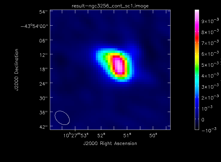
and again generate some statistics:
# In CASA
calstat=imstat(imagename='ngc3256_cont_sc1.image', region='', box='160,50,210,210')
rms=(calstat['rms'][0])
print '>> rms in continuum image: '+str(rms)
calstat=imstat(imagename='ngc3256_cont_sc1.image', region='')
peak=(calstat['max'][0])
print '>> Peak in continuum image: '+str(peak)
print '>> Dynamic range in continuum image: '+str(peak/rms)
The continuum image has improved a lot. The dynamic range is now ~110, whereas before it was only 34. The image peak flux density is ~9 mJy. We will write this new image to the file 'ngc3256_cont_sc1.image' to indicate that an iteration of self-calibration was performed.
# In CASA
imview(raster={'file': 'ngc3256_cont_sc1.image', 'colorwedge':T,
        'range':[-0.0003, 0.007], 'scaling':-1, 'colormap':'Rainbow 2'},
        out='ngc3256_cont_sc1.png', zoom=2)
Line cubes of the galaxy
We will start by running split to apply the latest self-calibration tables to the data column of the output measurement set.
# In CASA
os.system('rm -rf ngc3256_line_target_sc.ms*')
split(vis='ngc3256_line_target.ms', outputvis='ngc3256_line_target_sc.ms')
We will then subtract the continuum using the task uvcontsub:
# In CASA
uvcontsub(vis = 'ngc3256_line_target_sc.ms',
	  fitspw='0:20~53;71~120,1:70~120,2:20~120,3:20~120', solint ='inf',
	  fitorder = 1, fitmode = 'subtract')
- fitspw='0:20~53;71~120,1:70~120,2:20~120,3:20~120': To specify the spectral windows and channels to be used in the fit for the continuum. We avoid the spectral regions that include the CO and CN emission lines.
- solint ='inf': Timescale for the fit. Here we are electing one fit per scan
- fitorder = 1: We will fit a first-order polynomial to the continuum
- fitmode = 'subtract': Subtract the continuum from the data and store the result in the corrected_data column
Next, we will clean the CO (1-0) line emission:
# In CASA
os.system('rm -rf ngc3256_line_CO.*')
clean(vis='ngc3256_line_target_sc.ms', imagename='ngc3256_line_CO',
	spw='0:48~78', mode='channel', start='', nchan=31, width='',
	outframe='LSRK', restfreq='115.271201800GHz', mask=[53,50,87,83],
        niter=500, interactive=T, imsize=128, cell='1arcsec',
        weighting='briggs', robust=0.0)
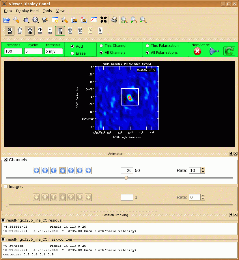
Notable parameters include:
- spw='0:48~78': To specify the CO (1-0) line emission alone
- mode='channel': To produce an image with different planes specified by the "start", "nchan", and "width" parameters
- start=, nchan=31, width=,: To include all 31 channels specified by spw, with no channel averaging
- outframe='LSRK': Shift the output reference frame to the local standard of rest
- restfreq='115.271201800GHz': The rest frequency of the CO line
- mask=[53,50,87,83]: The region in which to fit clean components (i.e., the source)
- niter=500, interactive=T: To do interactive cleaning with the viewer GUI
Using interactive=T the viewer will open when it is ready to start an interactive clean. Step through to the channels to see how extended the emission is. Then either use "All Channels" to define the same clean mask for all channels or select "This Channel" to select different masks for each channel. Once you have defined a polygon region, you need to double click inside it to save the mask region. You can use the "tape deck" to step through the channels again and check that the emission in all channels fits within the mask(s) you have created. To continue with clean use the "Next action" buttons in the green area on the Viewer Display GUI: The red X will stop clean where you are, the blue arrow will stop the interactive part of clean, but continue to clean non-interactively until reaching the stopping niter or threshold (whichever comes first), and the green arrow will clean until it reaches the "iterations" parameter on the left side of the green area.
When the cleaning has finished, you may want to inspect the resulting cube and and use the tape deck to play the cube as a movie. Use Spectral Profile in the Tools tab to make an integrated spectrum of the CO(1-0) emission.
# In CASA
viewer('ngc3256_line_CO.image')
The r.m.s noise level in the cube is XXX mJy per channel. The ALMA sensitivity calculator gives a noise level of XXX mJy, using 7 antennas and an integration time of 4 hours....
Next, we make the moment maps of the CO (1-0) emission using the task immoments:
# In CASA
os.system('rm -rf ngc3256_CO1-0.mom.*')
immoments(imagename='ngc3256_line_CO.image', moments=[0,1],
	chans='5~24', box='38,38,90,90', axis='spectral',
	includepix=[0.045, 10000], outfile='ngc3256_CO1-0.mom')
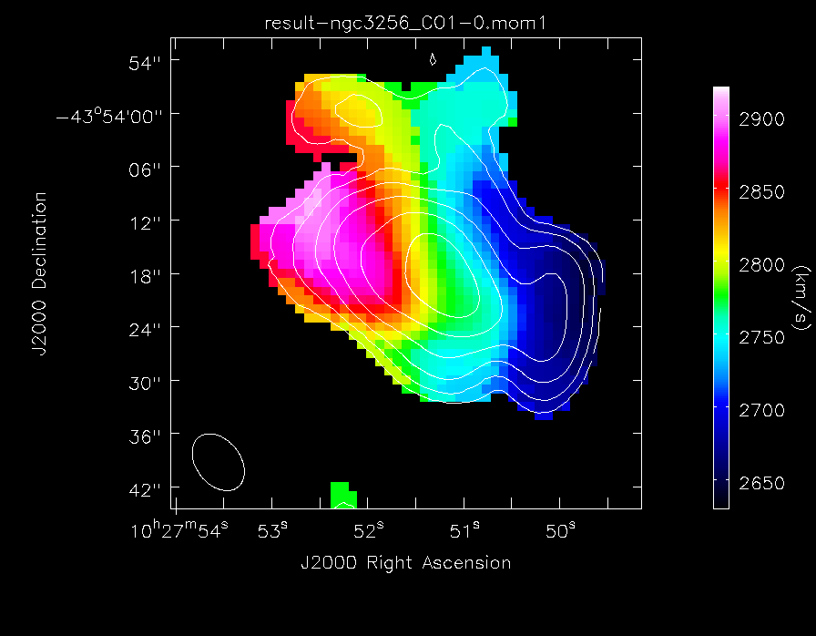
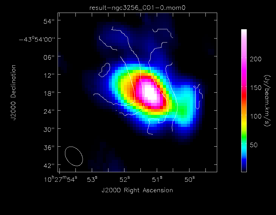
- moments=[0,1]: To specify that we wish to make the 0th and 1st moment maps, that is, the integrated emission map and the intensity weighted velocity field
- chans='5~24': These are the channels that show line emission and therefore the ones we want to use for the moment map
- box='38,38,90,90': To select a box region around the emission so as to not include any regions away from the galaxy
- axis='spectral': Indicates the moment axis, in this case 'spectral'
- includepix=[0.045, 10000]: To select which pixel values in the cube to include in the moments. We find these values by looking for the faintest believable emission in the cube
- outfile='ngc3256_CO1-0.mom': The output image base name
[NEED TO SAY SOMETHING ABOUT OUTPUT]
Make images of the CO(1-0) emission
# In CASA
imview(contour={'file': 'ngc3256_CO1-0.mom.integrated','range': []},
       raster={'file': 'ngc3256_CO1-0.mom.weighted_coord','range': [2630,2920],'colorwedge':T,
	       'colormap': 'Rainbow 2'},
       out='CO_velfield.png')
# In CASA
imview(contour={'file': 'ngc3256_CO1-0.mom.weighted_coord','levels':
               [2650,2700,2750,2800,2850,2900],'base':0,'unit':1},
       raster={'file': 'ngc3256_CO1-0.mom.integrated','colorwedge':T,
	       'colormap': 'Rainbow 2'},
       out='CO_map.png')
Next, we clean the CN high line emission:
# In CASA
os.system('rm -rf ngc3256_line_CNhi.*')
clean(vis='ngc3256_line_target_sc.ms', imagename='ngc3256_line_CNhi',
	outframe='LSRK', spw='1:50~76', start='', nchan=27, width='',
	restfreq='113.49097GHz', selectdata=T, mode='channel',
	niter=500, gain=0.1, psfmode='hogbom', mask=[53,50,87,83],
	interactive=True, imsize=128, cell='1arcsec',
	weighting='briggs', robust=0.0)
Make the moment maps of the CN (high) emission:
# In CASA
os.system('rm -rf ngc3256_CNhi.mom.*')
immoments( imagename='ngc3256_line_CNhi.image', moments=[0,1],
	chans='5~18', axis='spectral',box='38,38,90,90',
	includepix=[0.005, 10000], outfile='ngc3256_CNhi.mom')
Make images of the CN high emission:
# In CASA
imview(contour={'file': 'ngc3256_CNhi.mom.integrated','range': []},
       raster={'file': 'ngc3256_CNhi.mom.weighted_coord','range': [2630,2920],'colorwedge':T,
	       'colormap': 'Rainbow 2'},
       out='CNhi_velfield.png')
# In CASA
imview(contour={'file': 'ngc3256_CNhi.mom.weighted_coord','levels':
               [2650,2700,2750,2800,2850,2900],'base':0,'unit':1},
       raster={'file': 'ngc3256_CNhi.mom.integrated','colorwedge':T,
	       'colormap': 'Rainbow 2'},
       out='CNhi_map.png')
Clean the CN low emission:
# In CASA
os.system('rm -rf ngc3256_line_CNlo.*')
clean( vis='ngc3256_line_target_sc.ms', imagename='ngc3256_line_CNlo',
	outframe='LSRK', spw='1:29~54', start='', nchan=26, width='',
	restfreq='113.18666GHz', selectdata=T, mode='channel',
	niter=300, gain=0.1, psfmode='hogbom', mask=[53,50,87,83],
	interactive=True, imsize=128, cell='1arcsec',
	weighting='briggs', robust=0.0)
Make the moment maps of the CN (low) emission
# In CASA
os.system('rm -rf ngc3256_CNlo.mom.*')
immoments( imagename='ngc3256_line_CNlo.image', moments=[0,1],
	chans='8~18', axis='spectral', box='38,38,90,90',
	includepix=[0.003, 10000], outfile='ngc3256_CNlo.mom')
Make images of the CN low emission
# In CASA
imview(contour={'file': 'ngc3256_CNlo.mom.integrated','range': []},
       raster={'file': 'ngc3256_CNlo.mom.weighted_coord','range': [2630,2920],'colorwedge':T,
	       'colormap': 'Rainbow 2'},
       out='CNlo_velfield.png')
# In CASA
imview(contour={'file': 'ngc3256_CNlo.mom.weighted_coord','levels':
               [2650,2700,2750,2800,2850,2900],'base':0,'unit':1},
       raster={'file': 'ngc3256_CNlo.mom.integrated','colorwedge':T,
	       'colormap': 'Rainbow 2'},
       out='CNlo_map.png')