SMA CO Line Data 3.2: Difference between revisions
| Line 220: | Line 220: | ||
Next plot phase vs. channel. Here, we use plotms to iterate over the SMA baselines. While multiple subplots are not yet operational within plotms, you can view the individual phase vs. channel plots using the arrow buttons at the bottom right of the {{plotms}} window. By setting the '''xaxis''' parameter to 'frequency', we can see how the spectral windows overlap. Note the large discrepancy in phase for spw=4-7 on some baselines - this will be important later. | Next plot phase vs. channel. Here, we use plotms to iterate over the SMA baselines. While multiple subplots are not yet operational within plotms, you can view the individual phase vs. channel plots using the arrow buttons at the bottom right of the {{plotms}} window. By setting the '''xaxis''' parameter to 'frequency', we can see how the spectral windows overlap. Note the large discrepancy in phase for spw=4-7 on some baselines - this will be important later. | ||
[[File: | [[File:phaseVsfreqBaseline13.jpg|thumb| Phase vs. channel for the bandpass calibrator 3c454.3 and baseline 1-3.]] | ||
[[File:phaseVsfreqBaseline56.jpg|thumb| Phase vs. channel for the bandpass calibrator 3c454.3 and baseline 5-6.]] | |||
<source lang="python"> | <source lang="python"> | ||
| Line 372: | Line 373: | ||
Although in previous steps solutions were applied "on-the-fly", the data were not actually changed. Running {{applycal}} will fill the corrected data column in the ms. Again be careful with specification of '''gaintable''', and keeping the same order in '''spwmap''' and '''gainfield'''. This {{applycal}} is not necessary for later steps, but allows plotting of data calibration to this point. | Although in previous steps solutions were applied "on-the-fly", the data were not actually changed. Running {{applycal}} will fill the corrected data column in the ms. Again be careful with specification of '''gaintable''', and keeping the same order in '''spwmap''' and '''gainfield'''. This {{applycal}} is not necessary for later steps, but allows plotting of data calibration to this point. | ||
[[File: | [[File:ampvstimeFld9.jpg|thumb| Gain-corrected 3c454.3 data. Notice the few residual baseline-based problems.]] | ||
<source lang="python"> | <source lang="python"> | ||
Revision as of 21:37, 4 May 2011
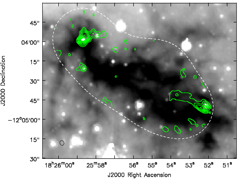
This script describes the data reduction of an SMA six-pointing mosaic of 12CO 2-1 emission in the infrared dark cloud G19.3+0.07. The CO line was placed in the USB. These data are from Brogan et al. in prep.; please do not use them for scientific purposes. This tutorial is based on the SMA CO Line Data script found in the CASA Scripts and Data page.
The data were previously filled in Miriad. A Tsys correction was applied, and the data were then written out in uvfits format. In this tutorial, CASA is used to read the uvfits files, and flag, calibrate, continuum subtract and image the data. Plotting for datasets with many spw such as SMA data (plotxy) can be slow. Where possible the new plotter plotms has been used.
You will need the tarball of the uvfits data, which can be downloaded here.
This tutorial uses the plotxy task in some places rather than plotms. Plotxy will eventually
be phased out, and this tutorial will be updated. In the meantime, this tutorial will work with
CASA Version 3.1.0.
Creating the measurement set from uvfits data
First, remove any files from previous run-throughs and unpack the tarball:
# In CASA
# Remove any files from previous run-throughs
os.system('rm -rf spw_fits.files')
os.system('tar xvf spw_fits_files.tar')
os.system('rm -rf g19_d2usb*')
Read in each uvfits file using the importuvfits filler (you need to set the upper range of the for loop to one more than you actually have, to satisfy ipython peculiarity). We create a list of the uvfits filenames in myfiles that will be used to create a single measurement set (ms).
# In CASA
os.system('rm -rf spw_ms_files')
os.system('mkdir spw_ms_files')
myfiles = []
for i in range(1,25):
    msfile = "spw_ms_files/g19_d2usb.spw"+str(i)+".ms"
    importuvfits(fitsfile="spw_fits_files/g19_d2usb.spw"+str(i),
                 vis=msfile)
    myfiles.append(msfile)
Using concat, create a single ms from the filenames listed in myfiles:
# In CASA
concat(vis=myfiles,concatvis='g19_d2usb.ms',timesort=True)
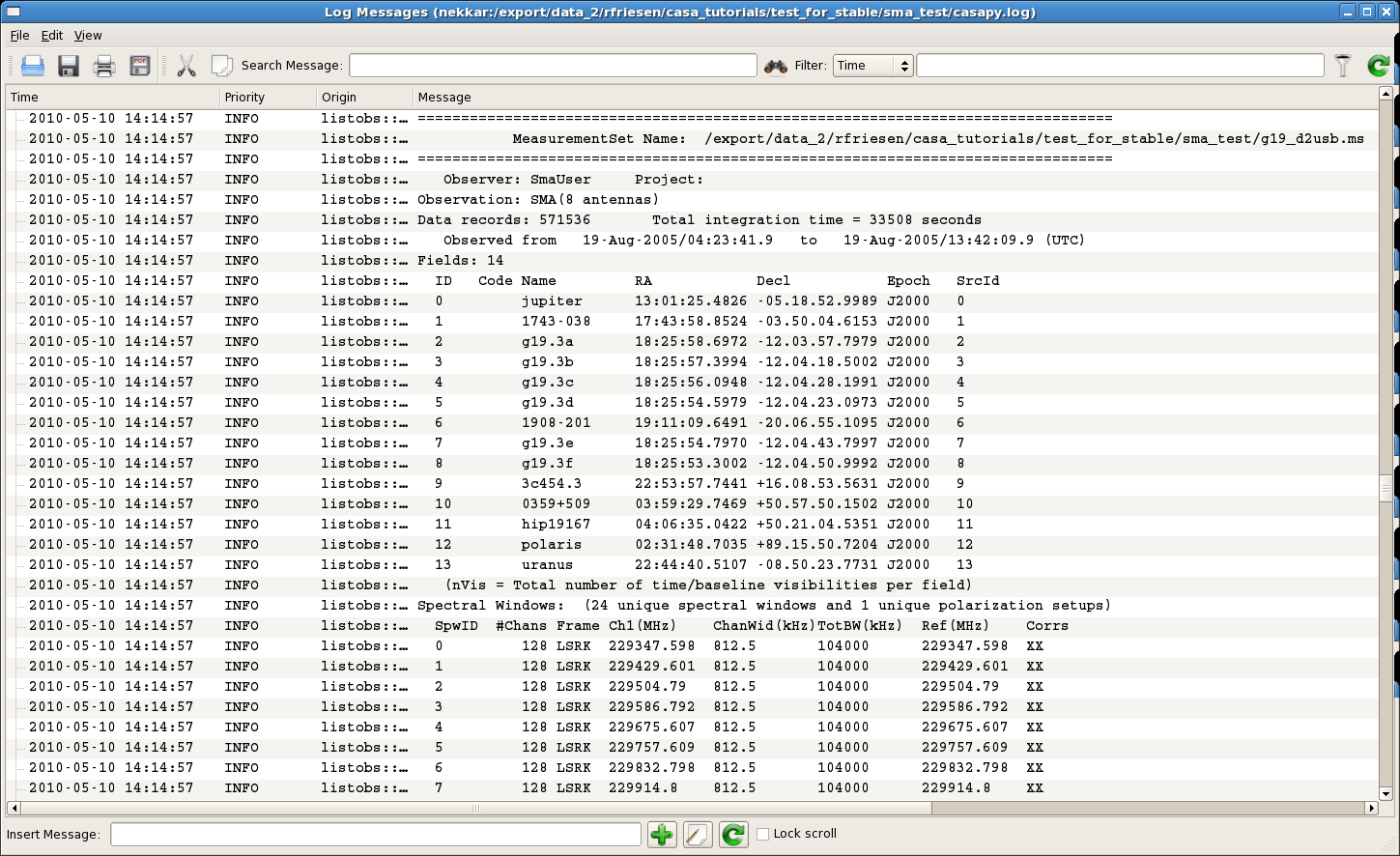
Finally, initialize the scratch columns using clearcal and use listobs to look at the contents of the measurement set (which appear in the CASA Log Messages window):
# In CASA
clearcal(vis='g19_d2usb.ms')
listobs(vis='g19_d2usb.ms',verbose=False)
##########################################
##### Begin Task: listobs            #####
listobs::::casa
================================================================================
MeasurementSet Name:  /export/data_2/rfriesen/casa_tutorials/test_for_stable/sma_co/sma_test/g19_d2usb.ms      MS Version 2
================================================================================
Observer: SmaUser     Project:
Observation: SMA(8 antennas)
Data records: 571536       Total integration time = 33508 seconds
Observed from   19-Aug-2005/04:23:41.9   to   19-Aug-2005/13:42:09.9 (UTC)
Fields: 14
      ID   Code Name          RA               Decl          Epoch   SrcId
      0         jupiter       13:01:25.48      -05.18.53.00  J2000   0
      1         1743-038      17:43:58.85      -03.50.04.62  J2000   1
      2         g19.3a        18:25:58.70      -12.03.57.80  J2000   2
      3         g19.3b        18:25:57.40      -12.04.18.50  J2000   3
      4         g19.3c        18:25:56.09      -12.04.28.20  J2000   4
      5         g19.3d        18:25:54.60      -12.04.23.10  J2000   5
      6         1908-201      19:11:09.65      -20.06.55.11  J2000   6
      7         g19.3e        18:25:54.80      -12.04.43.80  J2000   7
      8         g19.3f        18:25:53.30      -12.04.51.00  J2000   8
      9         3c454.3       22:53:57.74      +16.08.53.56  J2000   9
      10        0359+509      03:59:29.75      +50.57.50.15  J2000   10
      11        hip19167      04:06:35.04      +50.21.04.54  J2000   11
      12        polaris       02:31:48.70      +89.15.50.72  J2000   12
      13        uranus        22:44:40.51      -08.50.23.77  J2000   13
       (nVis = Total number of time/baseline visibilities per field)
Spectral Windows:(24 unique spectral windows and 1 unique polarization setups)
      SpwID  #Chans Frame Ch1(MHz)    ChanWid(kHz)TotBW(kHz)  Ref(MHz)    Corrs
      0         128 LSRK  229347.598  812.5       104000      229347.598  XX
      1         128 LSRK  229429.601  812.5       104000      229429.601  XX
      2         128 LSRK  229504.79   812.5       104000      229504.79   XX
      3         128 LSRK  229586.792  812.5       104000      229586.792  XX
      4         128 LSRK  229675.607  812.5       104000      229675.607  XX
      5         128 LSRK  229757.609  812.5       104000      229757.609  XX
      6         128 LSRK  229832.798  812.5       104000      229832.798  XX
      7         128 LSRK  229914.8    812.5       104000      229914.8    XX
      8         128 LSRK  230003.615  812.5       104000      230003.615  XX
      9         128 LSRK  230085.617  812.5       104000      230085.617  XX
      10        128 LSRK  230160.806  812.5       104000      230160.806  XX
      11        128 LSRK  230242.808  812.5       104000      230242.808  XX
      12        128 LSRK  230331.623  812.5       104000      230331.623  XX
      13        128 LSRK  230413.625  812.5       104000      230413.625  XX
      14        128 LSRK  230488.814  812.5       104000      230488.814  XX
      15        128 LSRK  230570.817  812.5       104000      230570.817  XX
      16        128 LSRK  230659.631  812.5       104000      230659.631  XX
      17        128 LSRK  230741.634  812.5       104000      230741.634  XX
      18        128 LSRK  230816.823  812.5       104000      230816.823  XX
      19        128 LSRK  230898.825  812.5       104000      230898.825  XX
      20        128 LSRK  230987.639  812.5       104000      230987.639  XX
      21        128 LSRK  231069.641  812.5       104000      231069.641  XX
      22        128 LSRK  231144.831  812.5       104000      231144.831  XX
      23        128 LSRK  231226.833  812.5       104000      231226.833  XX
The sources contained in this measurement set are:
Source Name        Description                                    ID
====================================================================
3c454.3            Bandpass and flux calibrator                    9
1743-038           Gain calibrator                                 1
1908-201           Gain calibrator                                 6
Uranus             Flux calibrator                                13
g19.7              Science target (6-pointing mosaic)    2,3,4,5,7,8
====================================================================
Other sources in the ms were not part of this program.
Initial inspection and flagging
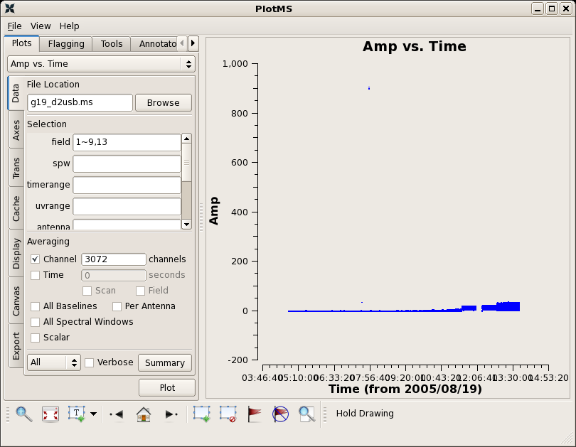
Use plotms to inspect the data.
# In CASA
clearstat()
plotms(vis="g19_d2usb.ms",xaxis="time",yaxis="amp",field='1~9,13',
       avgchannel='3072')
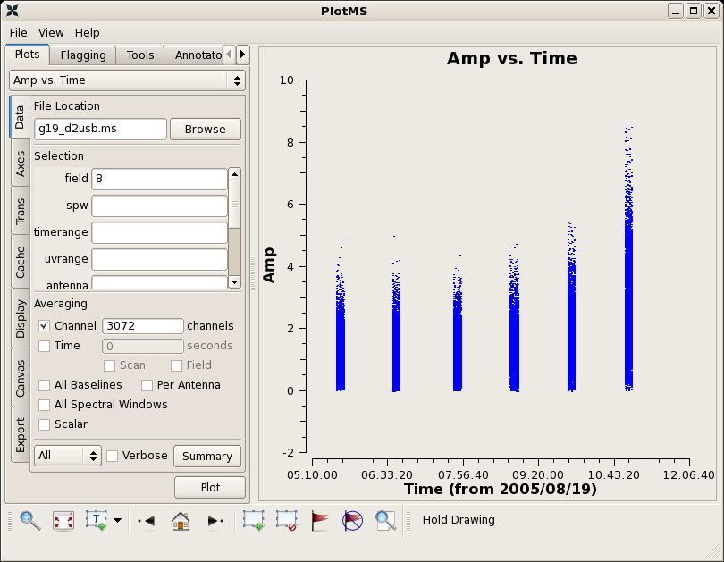
There are a few bad data points in this ms. You can use the locate features in plotms to find the bad data points on field 8 and antenna ids 1-2 and 0-2. Flagging can be done in plotms, or in a script using the flagdata command. Here we will do all flagging within the script.
Tip: locate gives antenna ids, but flagdata looks first at the name column. Since SMA antenna names are numbers, this can be confusing. The corresponding names are antennas 2-3 and 1-3, which you can check with listobs.
# In CASA
flagdata(vis='g19_d2usb.ms',mode='manualflag',field='8',spw='20~23',
	 timerange='07:52:45~07:52:47',antenna='2&3;1&3')
Plotting again shows that the bad data are gone:
# In CASA
clearstat()
plotms(vis="g19_d2usb.ms",xaxis="time",yaxis="amp",field='8',
       avgchannel='3072')
Tip: to confirm the data were flagged in plotms, you need to change selection in plot (for example change field and then change back), and then change back to original to clear the cache and force a re-read of the data.
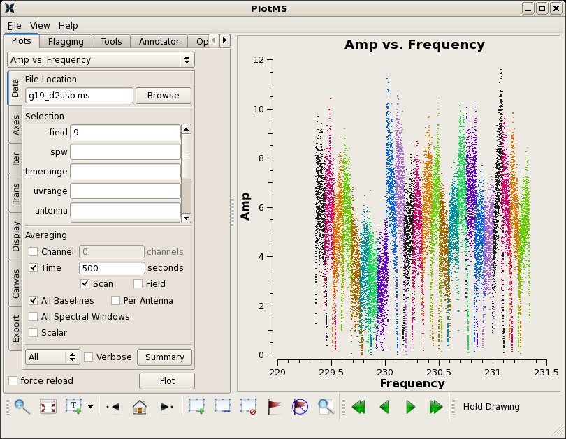
Make an inital amplitude vs. frequency plot of the bandpass calibrator 3c454.3, averaging the data together in time. Here, we colorize the points by spw in the plotms call using the coloraxis parameter. You can also do this under the 'Display' tab in the plotms window.
# In CASA
clearstat()
plotms(vis="g19_d2usb.ms",xaxis="freq",yaxis="amp",field="9",
       averagedata=True,avgscan=True,avgtime='500',avgbaseline=True,coloraxis="spw")
As you can see, SMA spw overlap by a fair amount. Here we will flag the first seven channels on either side of each spw to aid calibration:
# In CASA
default('flagdata')
flagdata(vis='g19_d2usb.ms', mode='manualflag',spw='0~23:0~6;121~127')
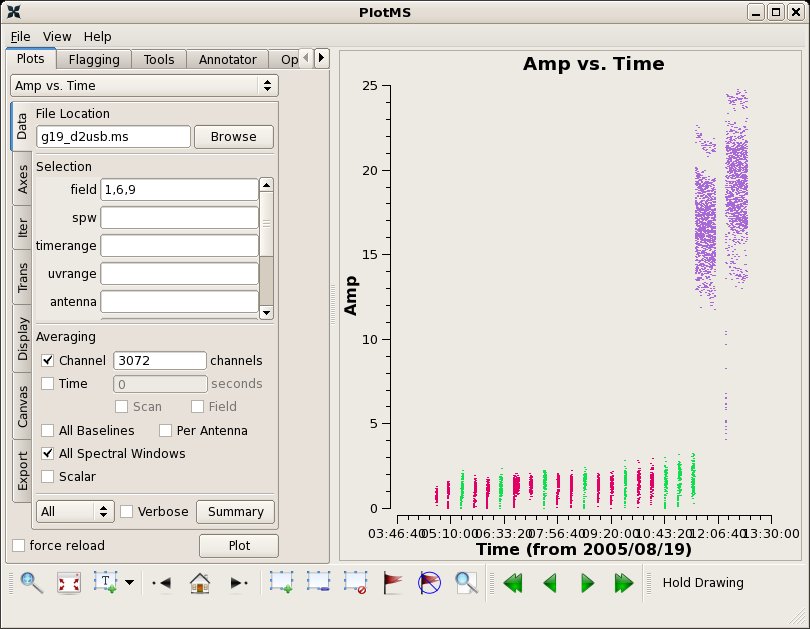
On many baselines the first integration of every scan is low. This can be seen with plotms.
# In CASA
clearstat()
plotms(vis="g19_d2usb.ms",xaxis="time",yaxis="amp",
       field='1,6,9',avgchannel='3072',avgspw=T,coloraxis="field")
Here, we have colored the points by field to see that the low amplitudes are found in the first integrations of many scans. These can also be flagged with flagdata. The integration time of these data is 30.9s. Note that more recent SMA data rarely show this problem.
# In CASA
flagdata(vis="g19_d2usb.ms",mode="quack",field='',
	 spw="0~23",quackinterval=40.0)
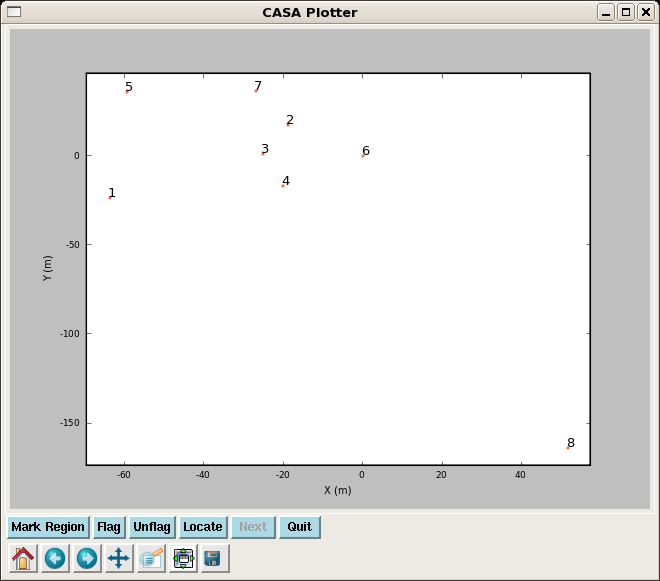
We can use plotxy to plot the antenna positions. For these observations, antenna 8 was in the barn for repair.
# In CASA
clearstat()
plotxy(vis="g19_d2usb.ms",xaxis="x")
Tip: after you run plotxy, run clearstat() before trying to run plotms or you will get a table lock.
Bandpass Calibration
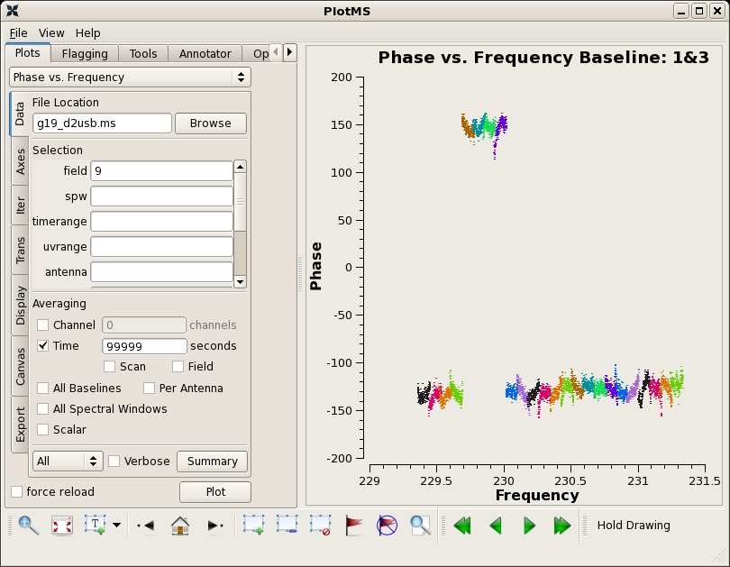
Next plot phase vs. channel. Here, we use plotms to iterate over the SMA baselines. While multiple subplots are not yet operational within plotms, you can view the individual phase vs. channel plots using the arrow buttons at the bottom right of the plotms window. By setting the xaxis parameter to 'frequency', we can see how the spectral windows overlap. Note the large discrepancy in phase for spw=4-7 on some baselines - this will be important later.
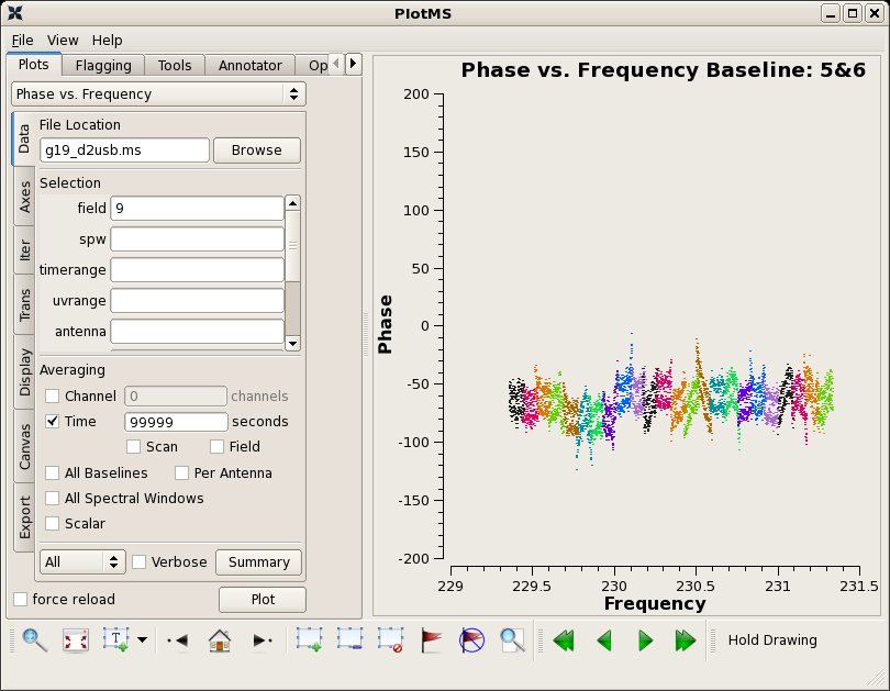
clearstat()
plotms(vis="g19_d2usb.ms",xaxis="frequency",yaxis="phase",
       ydatacolumn="data",field="9",iteraxis="baseline",
       averagedata=True,avgtime="99999",coloraxis="spw")
We can also use the slower plotxy to show multiple subplots in one panel. We set the plotxy parameter crossscan=T because there are two scans on 3c454.3.
# In CASA
clearstat()
plotxy(vis="g19_d2usb.ms",xaxis="channel",yaxis="phase",datacolumn="data",
       iteration="baseline",
       antenna="",spw="",field="9",
       averagemode="vector",width="1",timebin="all",
       crossscans=T,crossbls=False,stackspw=F,
       subplot=331,plotcolor="darkcyan",
       overplot=False,showflags=False,interactive=True,figfile="")
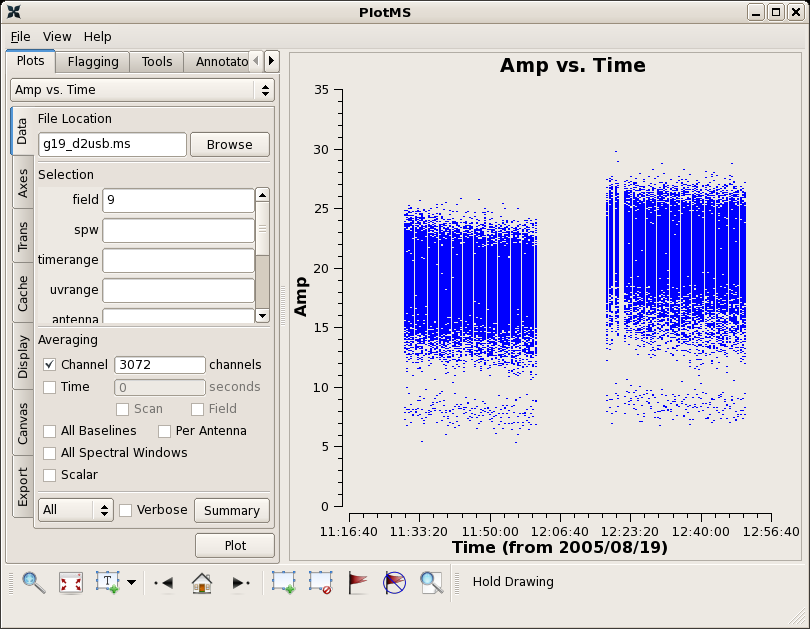
Now plot amplitude and phase as a function of time.
# In CASA
clearstat()
plotms(vis="g19_d2usb.ms",xaxis="time",yaxis="amp",field='9',
       avgchannel='3072')
The gap in the 3C454.3 observation is due to a pause to determine pointing solutions. The flags below catch times just before and after when the amplitudes and phase are off. This flagging could also have been accomplished interactively in plotms.
# In CASA
default('flagdata')
flagdata(vis="g19_d2usb.ms",field="9",timerange='12:16:58~12:19:00')
flagdata(vis="g19_d2usb.ms",field="9",timerange='12:08:00~12:09:30')
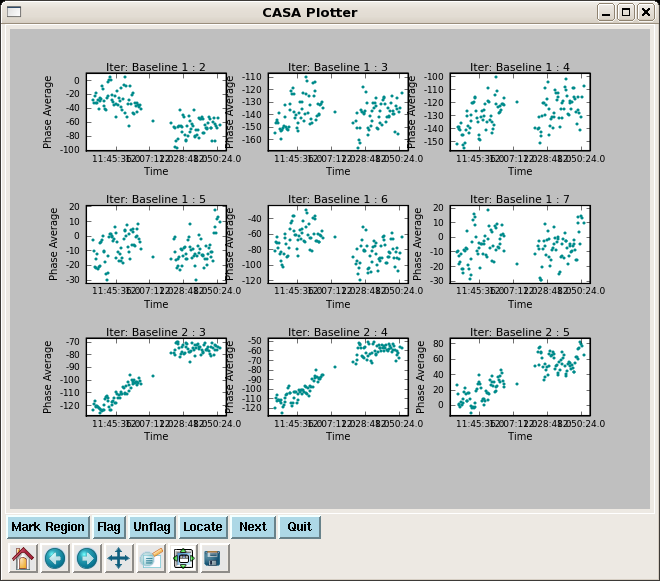
Here we plot phase vs. time for the bandpass calibrator 3c454.3. Be sure to use the arrow buttons in plotms to view all the baseline images. NOTE: plotms crashes if I try this
# In CASA
clearstat()
plotms(vis="g19_d2usb.ms",xaxis="time",yaxis="phase",ydatacolumn="data",
       field="9",spw="0~23",iteraxis="baseline",averagedata=True,avgspw=True)
This can also be done in a single panel using plotxy:
# In CASA
clearstat()
plotxy(vis="g19_d2usb.ms",xaxis="time",yaxis="phase",datacolumn="data",
       iteration="baseline", antenna="",spw="0~23",field="9",
       averagemode="vector",width="allspw",timebin="0",
       subplot=331,plotsymbol=".",
       multicolor="none",plotcolor="darkcyan",
       overplot=False,showflags=False,interactive=True,figfile="")
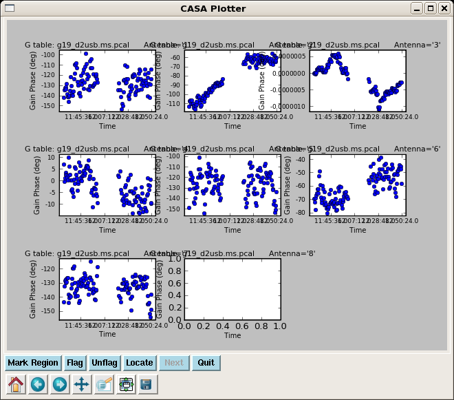
Start by determining an initial phase only solution for 3c454.3 using gaincal to take out major phase variations with time. For maximum sensitivity, we average all the spw together, with the exception of spw 4-7 which show large phase offsets from the other spw in phase vs. channel.
# In CASA
gaincal(vis='g19_d2usb.ms', caltable='g19_d2usb.ms.pcal',
	field='9', spw='0~3,8~23', gaintype='G', minsnr=2.0,
	refant='3', calmode='p',solint='int', combine='spw')
clearstat()
plotcal(caltable="g19_d2usb.ms.pcal",xaxis="time",yaxis="phase",
	field="9",antenna="",spw="",timerange="",subplot=331,
	overplot=False,clearpanel="Auto",iteration="antennas",
	plotsymbol="o",plotcolor="blue",showgui=True,figfile="")
Next we do a bandpass calibration. There are several possible solution types. A regular 'B' type solution can work well if you have lots of S/N on your bandpass calibrator. You may wish to make this table and compare to 'BPOLY' solution further down.
# In CASA
bandpass(vis='g19_d2usb.ms', caltable='g19_d2usb.ms.bpcal',
 	field='9', spw='0~23', bandtype='B', solint='inf', combine='scan',
 	refant='3', gaincurve=False, opacity=0.0,
 	gaintable='g19_d2usb.ms.pcal',spwmap=[0])
plotcal(caltable="g19_d2usb.ms.bpcal",xaxis="freq",yaxis="amp",
	field="9",antenna="",spw="",timerange="",subplot=311,
	overplot=False,clearpanel="Auto",iteration="antenna",
	plotsymbol="o",plotcolor="blue",showgui=True,figfile="")
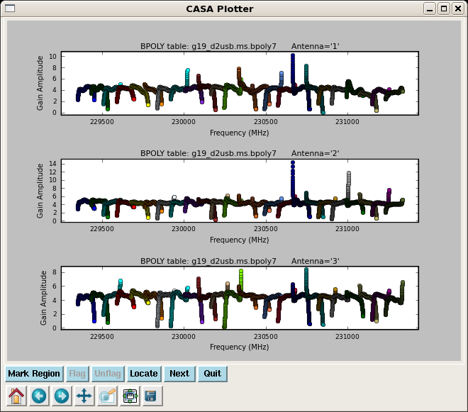
A polynomial bandpass solution is more sensitive than simply fitting a polynomial to the channel based solutions 'B' after the fact. For the mm/submm, where the S/N is often low on the bandpass calibrator, 'BPOLY' is often the best choice, but every dataset is different. You may especially need to play with the degamp and degphase parameters in bandpass. The parameter combine='scan' is needed to average together the two 3c454.3 scans. The spwmap=[0] is telling it to apply the phase solution that was found from the average of all spw to each spw before determining the bandpass solution.
# In CASA
bandpass(vis='g19_d2usb.ms', caltable='g19_d2usb.ms.bpoly7',
	field='9', spw='0~23', bandtype='BPOLY',
	solint='inf', combine='scan',
	refant='3', degamp=7, degphase=7,
	gaintable='g19_d2usb.ms.pcal',spwmap=[0])
clearstat()
plotcal(caltable="g19_d2usb.ms.bpoly7",xaxis="freq",yaxis="amp",
	field="9",antenna="",spw="",timerange="",subplot=311,
	overplot=False,clearpanel="Auto",iteration="antenna",
	plotsymbol="o",plotcolor="blue",showgui=True,figfile="")
Unfortunately, this kind of plot with many spw and colors takes a long time. Be patient for now, as it's being worked on. You can safely ignore where the solution gets large at edges of spw. This is showing where we flagged channels - this is also being worked on. Zoom in if necessary to see that inner portions are nice and flat.
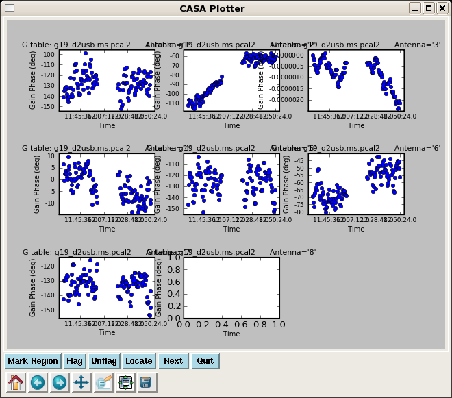
The next step is to apply the bandpass solution while re-calculating with gaincal the phase only solution for 3c454.3 on a short time interval (here, we use the integration time), but now including all spw (including 4~7 since antenna based solutions will have taken out phase vs.spw differences).
# In CASA
gaincal(vis='g19_d2usb.ms', caltable='g19_d2usb.ms.pcal2',
	field='9', spw='0~23', gaintype='G', minsnr=2.0,
	refant='3', calmode='p',solint='int', combine='spw',
	gaintable=['g19_d2usb.ms.bpoly7'])
clearstat()
plotcal(caltable="g19_d2usb.ms.pcal2",xaxis="time",yaxis="phase",
	field="9",antenna="",spw="",timerange="",subplot=331,
	overplot=False,clearpanel="Auto",iteration="antennas",
	plotsymbol="o",plotcolor="blue",showgui=True,figfile="")
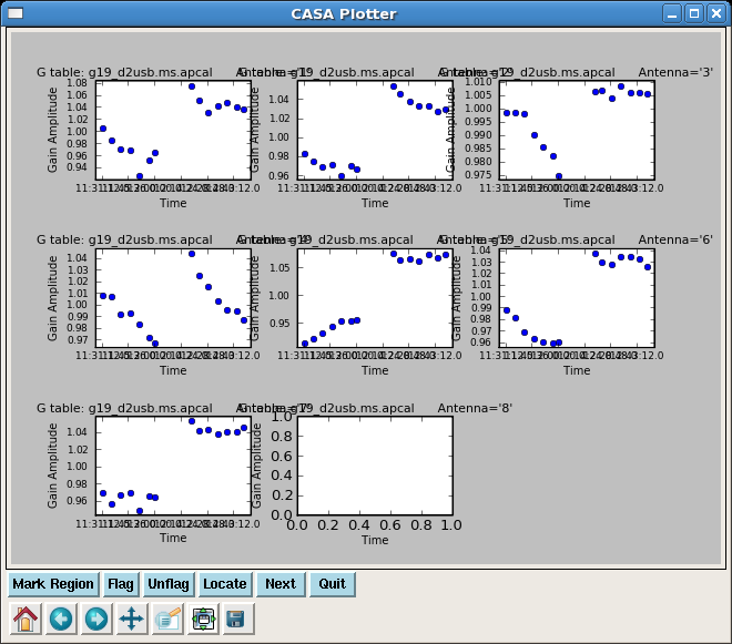
Next we apply the antenna based bandpass, and phase only solution to solve for amplitude solutions over a longer solint to increase the S/N. The spwmap=[[0],[]] tells gaincal that the pcal solution is independent of spw while the bpoly7 solution is per spw. spwmap order must be in the same order as the tables in gaintable.
# In CASA
gaincal(vis='g19_d2usb.ms', caltable='g19_d2usb.ms.apcal',
	field='9', spw='0~23', gaintype='G', minsnr=2.0,
	refant='3', calmode='a',solint='300s', combine='spw',
	gaintable=['g19_d2usb.ms.pcal2','g19_d2usb.ms.bpoly7'],
	spwmap=[[0],[]])
clearstat()
plotcal(caltable="g19_d2usb.ms.apcal",xaxis="time",yaxis="amp",
	field="9",antenna="",spw="",timerange="",subplot=331,
	overplot=False,clearpanel="Auto",iteration="antennas",
	plotsymbol="o",plotcolor="blue",showgui=True,figfile="")
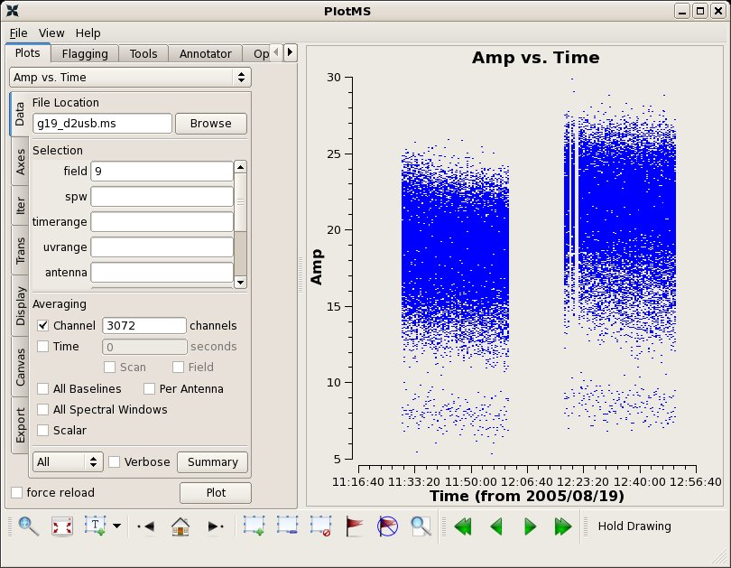
Although in previous steps solutions were applied "on-the-fly", the data were not actually changed. Running applycal will fill the corrected data column in the ms. Again be careful with specification of gaintable, and keeping the same order in spwmap and gainfield. This applycal is not necessary for later steps, but allows plotting of data calibration to this point.
# In CASA
applycal(vis='g19_d2usb.ms',spw='0~23', field='9',
	gaintable=['g19_d2usb.ms.pcal2','g19_d2usb.ms.apcal',
	'g19_d2usb.ms.bpoly7'],
	spwmap=[[0],[0],[]],gainfield=['9','9','9'])
clearstat()
plotms(vis="g19_d2usb.ms",xaxis="freq",yaxis="amp",
       ydatacolumn="corrected",iteraxis="baseline",
       spw="0~23",field="9",averagedata=True,avgtime='99999')
We can also view the data in a single plot using the slower plotxy:
# In CASA
plotxy(vis="g19_d2usb.ms",xaxis="channel",yaxis="amp",
       datacolumn="corrected",iteration="baseline",
       antenna='',spw="0~23",field="9",
       averagemode="vector",width="1",timebin="all",crossscans=T,
       crossbls=False,stackspw=False,extendflag=F,
       extendchan="",extendspw="",extendant="",extendtime="",
       plotcolor='darkcyan',subplot=331,
       multicolor="none",figfile="")
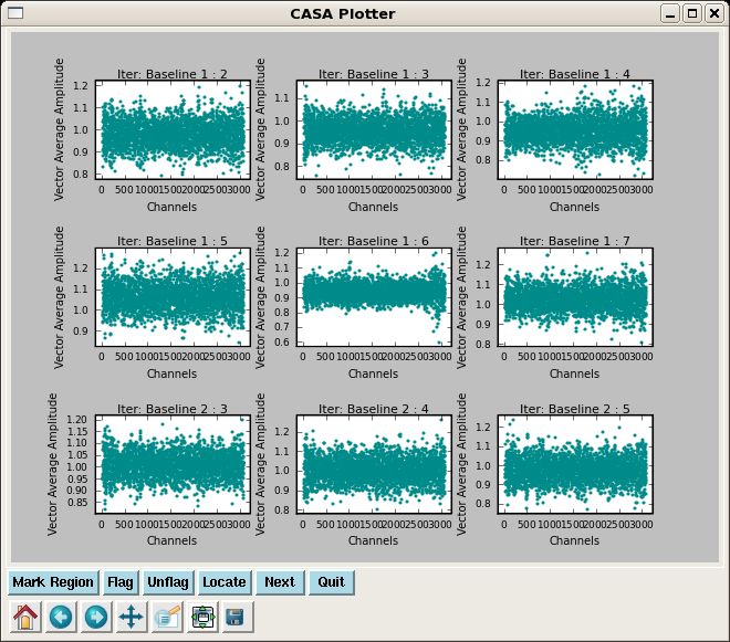
We can see by paging through the plots iterated over baseline (press the arrow button on the plotms display) that SMA data often show residual baseline based problems as a function of spw after antenna based bandpass (i.e. a few abnormally low amplitudes for a few spw on a few baselines). To fix this problem we need to do a baseline based amplitude only solution per spw, but we'll need to remove an overall normalization factor first by combining all spw (this option will be incorporated into blcal one day so that only one run is necessary). Note the significant change on baseline 1-6 in the following call to plotcal.
# In CASA
blcal(vis='g19_d2usb.ms', caltable='g19_d2usb.ms.blcal1',
	field='9', spw='0~23',solint='inf', combine='spw,scan',
	gaintable=['g19_d2usb.ms.pcal2','g19_d2usb.ms.apcal',
	'g19_d2usb.ms.bpoly7'],
	calmode='a',spwmap=[[0],[0],[]])
blcal(vis='g19_d2usb.ms', caltable='g19_d2usb.ms.blcal2',
	field='9', spw='0~23',solint='inf', combine='scan',
	gaintable=['g19_d2usb.ms.pcal2','g19_d2usb.ms.apcal',
	'g19_d2usb.ms.blcal1','g19_d2usb.ms.bpoly7',],
	calmode='a',spwmap=[[0],[0],[0],[]])
clearstat()
plotcal(caltable="g19_d2usb.ms.blcal2",xaxis="freq",yaxis="amp",
	field="9",antenna="",spw="",timerange="",subplot=511,
	overplot=False,clearpanel="Auto",iteration="antenna",
	plotsymbol="o",plotcolor="blue",showgui=True,figfile="")
Now we can do a new applycal including only the second blcal2 solution. Note that applycal overwrites the corrected column, so there is no need to clearcal. Like the antenna based bandpass the blcal solution is independent for each spw, so we set spwmap = [].
# In CASA
applycal(vis='g19_d2usb.ms',spw='0~23', field='9',
	gaintable=['g19_d2usb.ms.pcal2','g19_d2usb.ms.apcal',
	'g19_d2usb.ms.bpoly7','g19_d2usb.ms.blcal2'],
	spwmap=[[0],[0],[],[]],gainfield=['9','9','9','9'])
Note how flat the full bandpass is after all this calibration (be sure to view all baseline iterations using the plotms arrow button):
# In CASA
clearstat()
plotms(vis="g19_d2usb.ms",xaxis="freq",yaxis="amp",
       ydatacolumn="corrected",iteraxis="baseline",
       spw="0~23",field="9",averagedata=True,avgtime='99999')
Inspection of gain calibrators and setting the flux scale
Apply antenna and baseline based bandpass solutions to the gain calibrators with applycal:
# In CASA
clearstat()
applycal(vis='g19_d2usb.ms',spw='0~23', field='1,6',
	gaintable=['g19_d2usb.ms.bpoly7','g19_d2usb.ms.blcal2'],
	spwmap=[[],[]],gainfield=['9','9'])
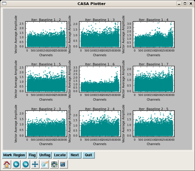
Have a look at the corrected data for both calibrators with channel vs. amplitude:
# In CASA
# First field 1:
clearstat()
plotxy(vis="g19_d2usb.ms",xaxis="channel",yaxis="amp",datacolumn="corrected",
       iteration="baseline", antenna="",spw="",field="1",
       averagemode="vector",width="1",timebin="all",
       subplot=331,plotsymbol=".",
       multicolor="none",plotcolor="darkcyan",
       overplot=False,showflags=False,interactive=True,figfile="")

# Next field 6:
clearstat()
plotxy(vis="g19_d2usb.ms",xaxis="channel",yaxis="amp",datacolumn="corrected",
       iteration="baseline", antenna="",spw="",field="6",
       averagemode="vector",width="1",timebin="all",
       subplot=331,plotsymbol=".",
       multicolor="none",plotcolor="darkcyan",
       overplot=False,showflags=False,interactive=True,figfile="")
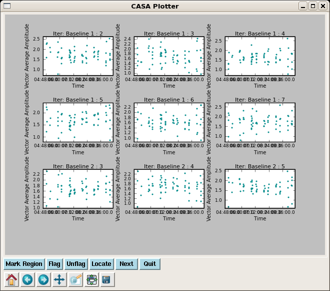
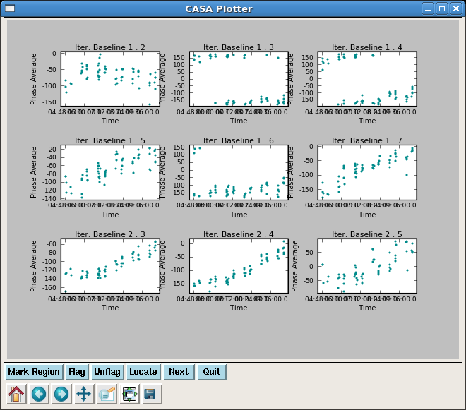
Have a look at the corrected data for both calibrators in phase and amplitude vs. time. For the moment, unfortunately, multicolor='field' doesn't work, so this is easiest to do separately. Note: new amplitudes are very low. Phases look fine.
# In CASA
# First, amplitude vs. time for field 1:
plotxy(vis="g19_d2usb.ms",xaxis="time",yaxis="amp",datacolumn="corrected",
       iteration="baseline", antenna="",spw="0~23",field="1",
       averagemode="vector",width="allspw",timebin="0",
       subplot=331,plotsymbol=".",
       multicolor="none",plotcolor="darkcyan",
       overplot=False,showflags=False,interactive=True,figfile="")

# Second, amplitude vs. time for field 6:
clearstat()
plotxy(vis="g19_d2usb.ms",xaxis="time",yaxis="amp",datacolumn="corrected",
       iteration="baseline", antenna="",spw="0~23",field="6",
       averagemode="vector",width="allspw",timebin="0",
       subplot=331,plotsymbol=".",
       multicolor="none",plotcolor="red",
       overplot=F,showflags=False,interactive=True,figfile="")

# Third, phase vs. time for field 1:
clearstat()
plotxy(vis="g19_d2usb.ms",xaxis="time",yaxis="phase",datacolumn="corrected",
       iteration="baseline", antenna="",spw="0~23",field="1",
       averagemode="vector",width="allspw",timebin="0",
       subplot=331,plotsymbol=".",
       multicolor="none",plotcolor="darkcyan",
       overplot=False,showflags=False,interactive=True,figfile="")

# Last, phase vs. time for field 6:
clearstat()
plotxy(vis="g19_d2usb.ms",xaxis="time",yaxis="phase",datacolumn="corrected",
       iteration="baseline", antenna="",spw="0~23",field="6",
       averagemode="vector",width="allspw",timebin="0",
       subplot=331,plotsymbol=".",
       multicolor="none",plotcolor="darkcyan",
       overplot=False,showflags=False,interactive=True,figfile="")
At the time of these observations, the calibrator J1911 had the most recent and relatively stable monitor data (SMA website), so we will use it for absolute flux calibration. In future tools for using resolved planets will be implemented.
1911-201
1mm   17 Jul 2005 11:38   SMA      274.5    1.88 +/-  0.13    mgurwell
1mm   05 Sep 2005 08:10   SMA      221.4    1.99 +/-  0.12    mgurwell
# In CASA
setjy(vis='g19_d2usb.ms', field='6', spw='0~23', fluxdensity=[2.0,0.,0.,0.])
Final gain and flux calibration for all calibrators
Next, we calculate two separate phase solutions from the data. To avoid decorrelation of the amplitude, the phase solutions fed to the amplitude calibration step should be at the shortest solint your S/N can support. Typically this will be the integration time.
Note: get the following warning: 2011-05-04 19:04:29 WARN gaincal:::: Phase continuity broken at 2005/08/19/06:50:49.3 (Spw=0, Fld=1, pol=0) 2011-05-04 19:04:29 WARN gaincal::::+ due to lack of overlapping antennas with previous interval.
# In CASA
gaincal(vis='g19_d2usb.ms', caltable='g19_d2usb.ms.allpcal',
	field='1,6,9', spw='0~23', gaintype='G', minsnr=2.0,
	refant='3', calmode='p',solint='int', combine='spw',
	gaintable=['g19_d2usb.ms.bpoly7','g19_d2usb.ms.blcal2'],
	spwmap=[[],[]])
Unless you chose to do some more sophisticated smoothing, the phase solutions applied to your target might as well be on the scan time of your phase calibrator(s). Without combine='scan', the solution will not cross scan boundaries even though solint='inf'. This is an easy way to "manually" interpolate.
# In CASA
gaincal(vis='g19_d2usb.ms', caltable='g19_d2usb.ms.allpcalscan',
	field='1,6,9', spw='0~23', gaintype='G', minsnr=2.0,
	refant='3', calmode='p',solint='inf', combine='spw',
	gaintable=['g19_d2usb.ms.bpoly7','g19_d2usb.ms.blcal2'],
	spwmap=[[],[]])
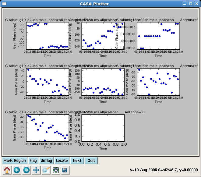
Plot the phase solutions of the phase calibrators. Can repeat for both short and long solution intervals.
# In CASA
clearstat()
plotcal(caltable="g19_d2usb.ms.allpcalscan",xaxis="time",yaxis="phase",
	field="1,6",antenna="",spw="",timerange="",subplot=331,
	overplot=False,clearpanel="Auto",iteration="antennas",
	plotsymbol="o",plotcolor="blue",showgui=True,figfile="")
Amplitude calibration with longer solint and applying short solint phase solution.
# In CASA
gaincal(vis='g19_d2usb.ms', caltable='g19_d2usb.ms.allapcal',
	field='1,6,9', spw='0~23', gaintype='G', minsnr=2.0,
	refant='3', calmode='ap',solint='300s', combine='spw',
	gaintable=['g19_d2usb.ms.allpcal','g19_d2usb.ms.bpoly7',
	'g19_d2usb.ms.blcal2'],spwmap=[[0],[],[]])
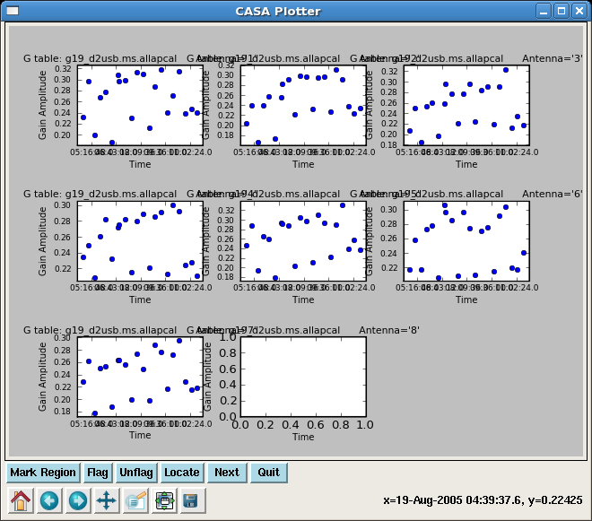
Plot the amplitude solutions:
# In CASA
clearstat()
plotcal(caltable="g19_d2usb.ms.allapcal",xaxis="time",yaxis="amp",
	field="1,6",antenna="",spw="",timerange="",subplot=331,
	overplot=False,clearpanel="Auto",iteration="antennas",
	plotsymbol="o",plotcolor="blue",showgui=True,figfile="")
Derive the absolute flux calibration using fluxscale (based on setjy above):
# In CASA
fluxscale(vis='g19_d2usb.ms',caltable='g19_d2usb.ms.allapcal',
	fluxtable='g19_d2usb.ms.fluxcal',reference='6')
Apply final calibrations
The final application of calibration for each source is done independently below. Flux densities from SMA flux monitoring are provided as checks of the absolute flux calibration.
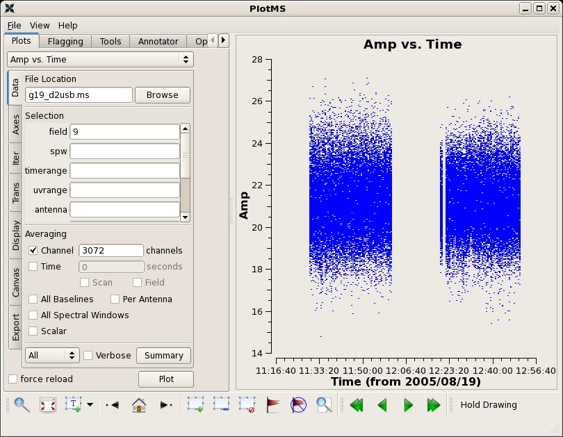
# In CASA
applycal(vis='g19_d2usb.ms',spw='0~23', field='9',
	gaintable=['g19_d2usb.ms.allpcal','g19_d2usb.ms.fluxcal',
	'g19_d2usb.ms.bpoly7','g19_d2usb.ms.blcal2'],spwmap=[[0],[0],[],[]],
	gainfield=['9','9','9','9'])
clearstat()
plotms(vis="g19_d2usb.ms",xaxis="time",yaxis="amp",field='9',
       avgchannel='3072',ydatacolumn='corrected')
3C454.3
1mm   19 Aug 2005 16:01   SMA      225.3   27.36 +/-  1.37    mgurwell
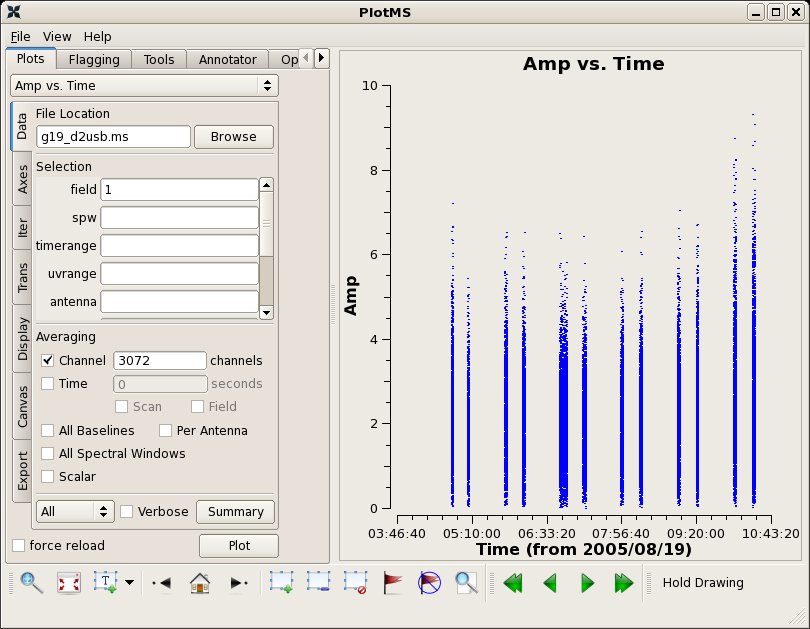
# In CASA
applycal(vis='g19_d2usb.ms',spw='0~23', field='1',
	gaintable=['g19_d2usb.ms.allpcal','g19_d2usb.ms.fluxcal',
	'g19_d2usb.ms.bpoly7','g19_d2usb.ms.blcal2'],spwmap=[[0],[0],[],[]],
	gainfield=['1','1','9','9'])
clearstat()
plotms(vis="g19_d2usb.ms",xaxis="time",yaxis="amp",field='1',
       avgchannel='3072',ydatacolumn='corrected')
J1743-038
1mm   26 Aug 2005 06:05   SMA      225.6    1.71 +/-  0.09    mgurwell
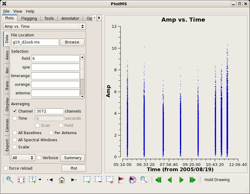
# In CASA
applycal(vis='g19_d2usb.ms',spw='0~23', field='6',
	gaintable=['g19_d2usb.ms.allpcal','g19_d2usb.ms.fluxcal',
	'g19_d2usb.ms.bpoly7','g19_d2usb.ms.blcal2'],spwmap=[[0],[0],[],[]],
	gainfield=['6','6','9','9'])
clearstat()
plotms(vis="g19_d2usb.ms",xaxis="time",yaxis="amp",field='6',
       avgchannel='3072',ydatacolumn='corrected')
J1911-201
1mm   17 Jul 2005 11:38   SMA      274.5    1.88 +/-  0.13    mgurwell
1mm   05 Sep 2005 08:10   SMA      221.4    1.99 +/-  0.12    mgurwell
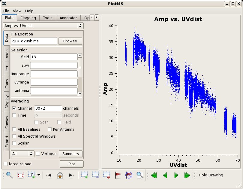
Since Uranus is resolved we apply the solutions from 3C454.3 to achieve at least some reduction in instrumental gain variations.
# In CASA
applycal(vis='g19_d2usb.ms',spw='0~23', field='13',
	gaintable=['g19_d2usb.ms.allpcal','g19_d2usb.ms.fluxcal',
	'g19_d2usb.ms.bpoly7','g19_d2usb.ms.blcal2'],spwmap=[[0],[0],[],[]],
	gainfield=['9','9','9','9'])
clearstat()
plotms(vis="g19_d2usb.ms",xaxis="uvdist",yaxis="amp",field='13',
       avgchannel='3072',ydatacolumn='corrected')
A UV-distance plot of the expected flux of Uranus can be obtained from the SMA webpage. In future we will implement tools to use planets for absolute flux calibration.
# In CASA
applycal(vis='g19_d2usb.ms',spw='0~23', field='2,3,4,5,7,8',
	gaintable=['g19_d2usb.ms.allpcalscan','g19_d2usb.ms.fluxcal',
	'g19_d2usb.ms.bpoly7','g19_d2usb.ms.blcal2'],spwmap=[[0],[0],[],[]],
	gainfield=['1,6','1,6','9','9'])
Split off target data for further inspection
# In CASA
split(vis="g19_d2usb.ms",outputvis='g19_d2usb_targets.ms',
      field="2,3,4,5,7,8")
To reinitialize the scratch columns for use by later tasks, we need to run clearcal for the new dataset. Then run listobs to check the target data names.
# In CASA
clearcal(vis='g19_d2usb_targets.ms')

listobs(vis="g19_d2usb_targets.ms",verbose=F)
ID   Code Name          Right Ascension  Declination   Epoch
0         g19.3a        18:25:58.70      -12.03.57.80  J2000
1         g19.3b        18:25:57.40      -12.04.18.50  J2000
2         g19.3c        18:25:56.09      -12.04.28.20  J2000
3         g19.3d        18:25:54.60      -12.04.23.10  J2000
4         g19.3e        18:25:54.80      -12.04.43.80  J2000
5         g19.3f        18:25:53.30      -12.04.51.00  J2000
Tip: After splitting, the "corrected" data column in the original vis file will become the "data" and "corrected" columns and the field IDs are renumbered.
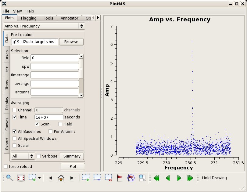
# In CASA
clearstat()
plotms(vis='g19_d2usb_targets.ms',xaxis="frequency",yaxis="amp",field='0',
       avgtime='1e7',avgscan=True,avgbaseline=True)

clearstat()
plotms(vis='g19_d2usb_targets.ms',xaxis="time",yaxis="amp",field='',
       avgchannel='3072',avgspw=True)
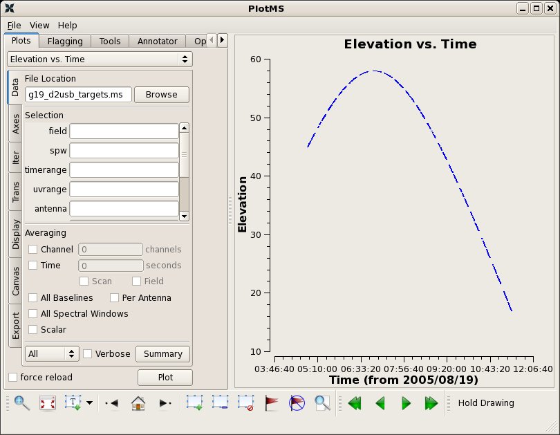
Data at times > 11:04:00 show lots of scatter: the elevation of these data are very low and are worth flagging. One can plotms with xaxis="time", yaxis="elevation" to see this.
# In CASA
clearstat()
plotms(vis='g19_d2usb_targets.ms',xaxis="time",yaxis="elevation",field='')
# In CASA
flagdata(vis="g19_d2usb_targets.ms",field="",timerange='>11:04:00')
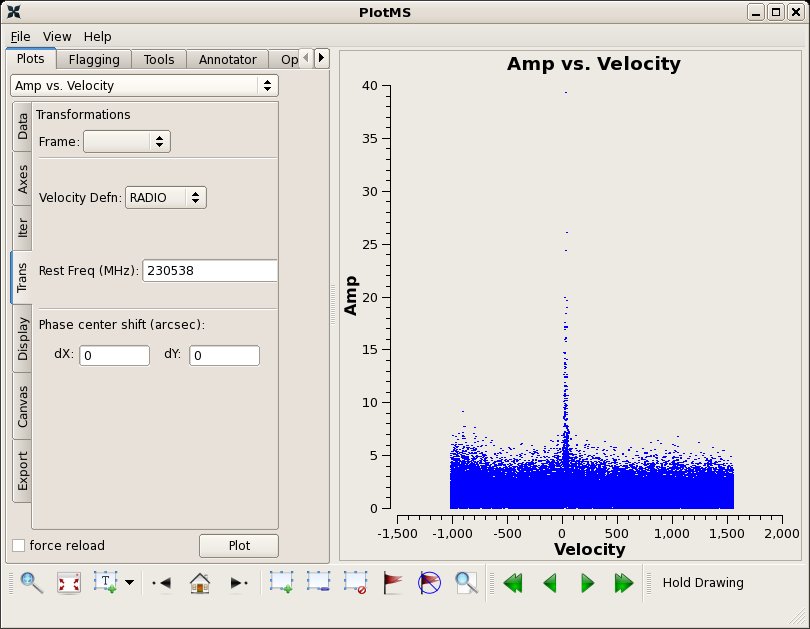
Note that because the Doppler tracked frequency was 13CO (+ 10GHz in the USB), the velocity diplayed in plotms will not be correct unless you set the rest frequency to the line of interest. You can do this in the plotms call, or in the Trans tab in the plotms display:
CO(2-1) restfreq=230.53797 GHz
# In CASA
clearstat()
plotms(vis="g19_d2usb_targets.ms",xaxis="velocity",yaxis="amp",
       ydatacolumn="data",selectdata=True,
       spw="0~23",field="0",averagedata=True,avgtime='99999',
       transform=True,restfreq="230.53797GHz")
The other weak line detected in this sideband is not visible in a vector average plot.
A-CH3OH (8 -1 8 0 -- 7 +0 7 0) 229.75876 GHz
Continuum imaging and subtraction
Next we want to make a continuum-free line dataset. We use field 0 to pick the line free spw, and can see that the line is confined to spws 13~15 by colorizing by spw:
# In CASA
clearstat()
plotms(vis="g19_d2usb_targets.ms",xaxis="freq",yaxis="amp",
       ydatacolumn="data",selectdata=True,coloraxis="spw",
       spw="0~23",field="0",averagedata=True,avgtime='99999')
Copy the original ms in case something goes wrong. Currently uvcontsub2 will change the input model and corrected columns, so it's best to make a back up. This behavior will change in future.
# In CASA
os.system('cp -r g19_d2usb_targets.ms g19_d2usb_targets_line.ms')
Now use new task uvcontsub2 to subtract the continuum. Unlike uvcontsub, this task will subtract the continuum estimate for spw that are not in the fitspw list. In future releases uvcontsub2 will likely replace uvcontsub. Setting fitspw='0~12,16~23' tells uvcontsub2 where to fit the continuum emission.
# In CASA
uvcontsub2(vis='g19_d2usb_targets_line.ms',fitspw='0~12,16~23',
	  solint='int',combine='spw',spw='0~23',
          fitorder=1)
The directory g19_d2usb_targets_line.ms.contsub/ contains the continuum-subtracted line data. We will make a separate dataset, g19_d2usb_targets_line.ms.cont, using the split task for imaging. Because the continuum model subtracted from the line dataset by uvcontsub2 is necessarily a smoothed fit, images made with it are liable to have their field of view reduced in some strange way. Images of the continuum should be made by simply excluding the line channels, as we show here.
# In CASA
split(vis='g19_d2usb_targets.ms',outputvis='g19_d2usb_targets_line.ms.cont',
      datacolumn='data',field='',spw='0~12,16~23')
Next we image the continuum data:
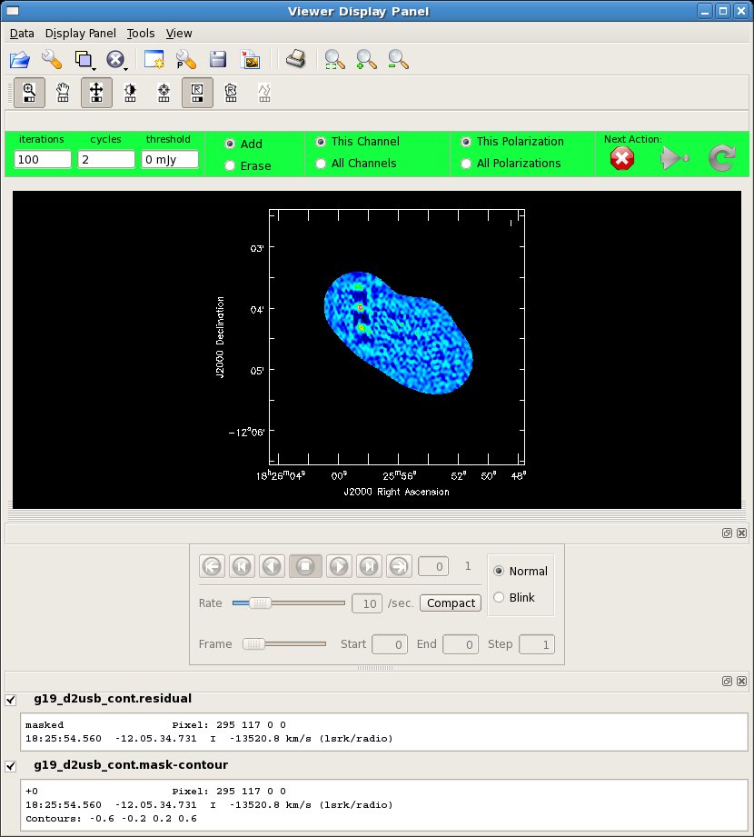
Tip: for sparse mosaics like this one, the subparameter ftmachine='ft' will typically give better results than the default ftmachine='mosaic'. For Nyquist sampled mosaics, ftmachine='mosaic' is the best choice, and the only choice for heterogeneous arrays. Also note that in a mosaic, the rms noise changes as a function of position. Therefore, the rms noise that you calculate from the radiometer equation is only valid where the combined primary beam response of the mosaic is near one. clean weights the decision of what to clean next by the primary beam response function (PBRF), so emission near PBRF=1 will be cleaned faster than elsewhere. Thus, if you have emission away from the "sweet spot(s)" you will need to clean to a threshold lower than you might expect from the anticipated rms noise. Development is on-going to provide other options which may work better for the case of strong emission near image boundaries.
# In CASA
clean(vis='g19_d2usb_targets_line.ms.cont',imagename='g19_d2usb_cont',
      field='',spw='0~23',
      mode='mfs',niter=200,gain=0.1,threshold=0.0,
      psfmode='clark',imagermode='mosaic',scaletype='SAULT',
      ftmachine='ft',
      interactive=T,imsize=500,cell="0.5arcsec",
      phasecenter="J2000 18h25m56.09 -12d04m28.20",
      pbcor=F,minpb=0.2)

viewer('g19_d2usb_cont.image')
Here you can see one stronger continuum source to the NE (18:25:58.5 -12:03:58.9) and one weak one to the SW (18:25:52, -12:04:53). The weak one is only visible after one round of cleaning. Because the mosaic is sparse you should make a clean mask to get the best cleaned image.
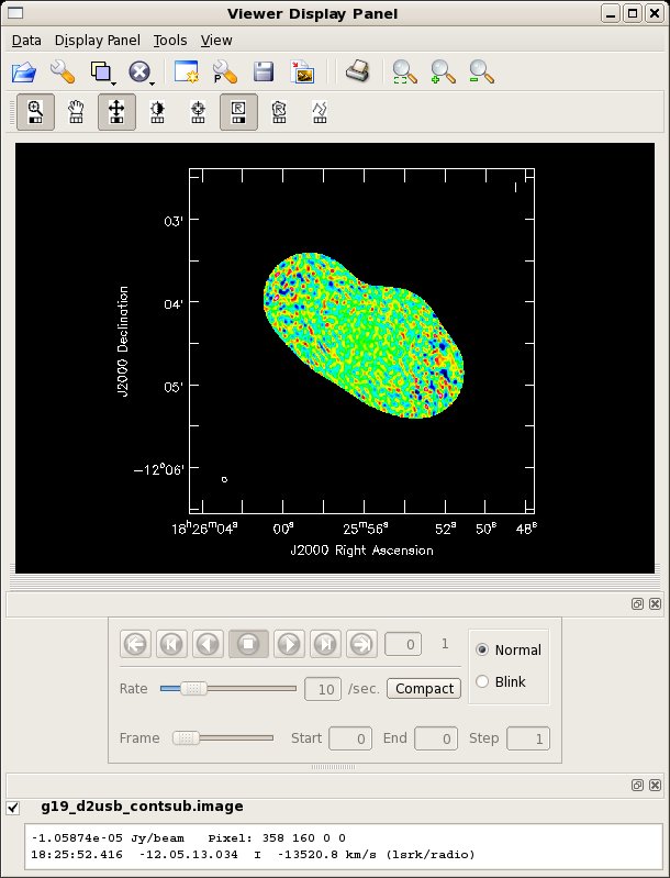
Make a dirty image of the continuum subtracted data, excluding the spws which contain line emission. You should see nothing but noise.
# In CASA
clean(vis='g19_d2usb_targets_line.ms.contsub',imagename='g19_d2usb_contsub',
      field='',spw='0~12,16~23',
      mode='mfs',niter=0,gain=0.1,threshold=0.0,
      psfmode='clark',imagermode='mosaic',scaletype='SAULT',
      ftmachine='ft',
      interactive=F,imsize=500,cell="0.5arcsec",
      phasecenter="J2000 18h25m56.09 -12d04m28.20",
      pbcor=F,minpb=0.2)
You can look at the image with the viewer; you should see nothing because the continuum has been subtracted.
# In CASA
viewer('g19_d2usb_contsub.image')
Spectral line imaging
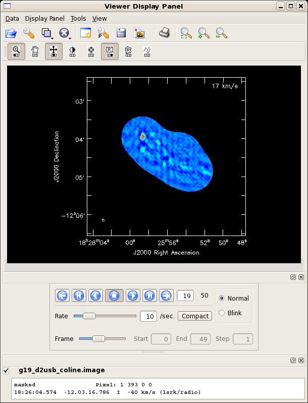
This image selects a channel range suitable to image the 12CO(2-1) line. Notice the use of the restfreq parameter to get the velocity scale correct.
# In CASA
clean(vis='g19_d2usb_targets_line.ms.contsub',imagename='g19_d2usb_coline',
      field='',spw='',
      mode='velocity',start='-40km/s',nchan=50,width='3km/s',
      interpolation='linear',
      niter=1000,gain=0.1,threshold=0.2,
      psfmode='clark',imagermode='mosaic',scaletype='SAULT',
      ftmachine='ft',restfreq='230.53797GHz',
      interactive=T,npercycle=400,
      imsize=500,cell="0.5arcsec",
      phasecenter="J2000 18h25m56.09 -12d04m28.20",
      pbcor=F,minpb=0.15)
It is essential to run with interactive=T and make a clean mask. A clean mask is available in the original data directory spw_fits_files. To use the pre-made mask, run:
# In CASA
clean(vis='g19_d2usb_targets_line.ms.contsub',imagename='g19_d2usb_coline',
      field='',spw='',
      mode='velocity',start='-40km/s',nchan=50,width='3km/s',
      niter=1000,gain=0.1,threshold=0.2,
      psfmode='clark',imagermode='mosaic',scaletype='SAULT',
      ftmachine='ft',restfreq='230.53797GHz',
      interactive=F,npercycle=400,
      imsize=500,cell="0.5arcsec",
      mask='spw_fits_files/coline.mask',
      phasecenter="J2000 18h25m56.09 -12d04m28.20",
      pbcor=F,minpb=0.15)
View the image produced:
# In CASA
viewer('g19_d2usb_coline.image')
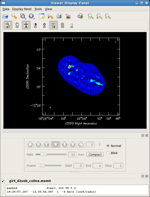
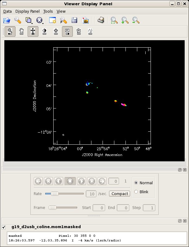
Now make 0th and 1st moment maps.
# In CASA
# 0th moment map
immoments(imagename='g19_d2usb_coline.image',moments=[0],axis='spectral',
	  chans='12~39',outfile='g19_d2usb_coline.mom0')

viewer('g19_d2usb_coline.mom0')

# 1st moment map
immoments(imagename='g19_d2usb_coline.image',moments=[1],axis=3,
	  chans='12~39',outfile='g19_d2usb_coline.mom1',
	  includepix=[0,2])

immath(outfile='g19_d2usb_coline.mom1masked',mode='evalexpr',
       expr='"g19_d2usb_coline.mom1"["g19_d2usb_coline.mom0">9]')

viewer('g19_d2usb_coline.mom1masked')
By clicking on the "folder" icon in the viewer window you can bring up the moment0 as a contour image. The strange appearance of the the moment1 map toward the NE source is probably due to more than one outflow being superposed.
Note that one could and should correct the image for the primary beam response using immath to divide the image by the .flux image. One would then need to make a mask for the moment images in order to hide the ugly stuff at the edges.
Last checked on CASA Version 3.2.0.