Data flagging with plotms: Difference between revisions
| Line 77: | Line 77: | ||
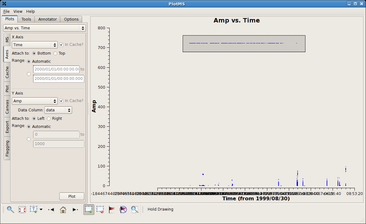
* Highlight the data to be flagged using the '''Mark Regions''' [[Image:MarkRegionsButton.png]] tool. | * Highlight the data to be flagged using the '''Mark Regions''' [[Image:MarkRegionsButton.png]] tool. | ||
* Flag the data in the highlighted region using the '''Flag''' [[Image:FlagThoseData.png]] tool. | * Flag the data in the highlighted region using the '''Flag''' [[Image:FlagThoseData.png]] tool. | ||
The figure at right shows a highlighted region selected using the '''Mark Regions''' tool. | |||
</div> | </div> | ||
Revision as of 19:19, 1 December 2009
Casaplotms is (currently) a standalone tool to inspect and edit measurement sets. This tutorial demonstrates how to use casaplotms to edit a multisource continuum data set: VLA program AU079, which consists of L-band (20 cm) continuum observations of galaxies and calibrator sources. It is the same data set used in the Imaging Flanking Fields tutorial, as well as the Data flagging with viewer tutorial.
Loading the Measurement Set into Casaplotms
As described in the Imaging Flanking Fields tutorial, the data may be loaded into CASA using the importvla command. The following commands import the data into the measurement set au079.ms and exit CASA to the command line.
# import the glob command for filename searching with wildcards
from glob import glob

# Define the list of files for reading. Use glob to perform wildcard matching with VLA archive filenames.
fileList = glob('AU079_*.xp?')

importvla(archivefiles=fileList,vis='au079.ms')
exit()
Now start up casaplotms from the command line.
# in bash
casaplotms
|
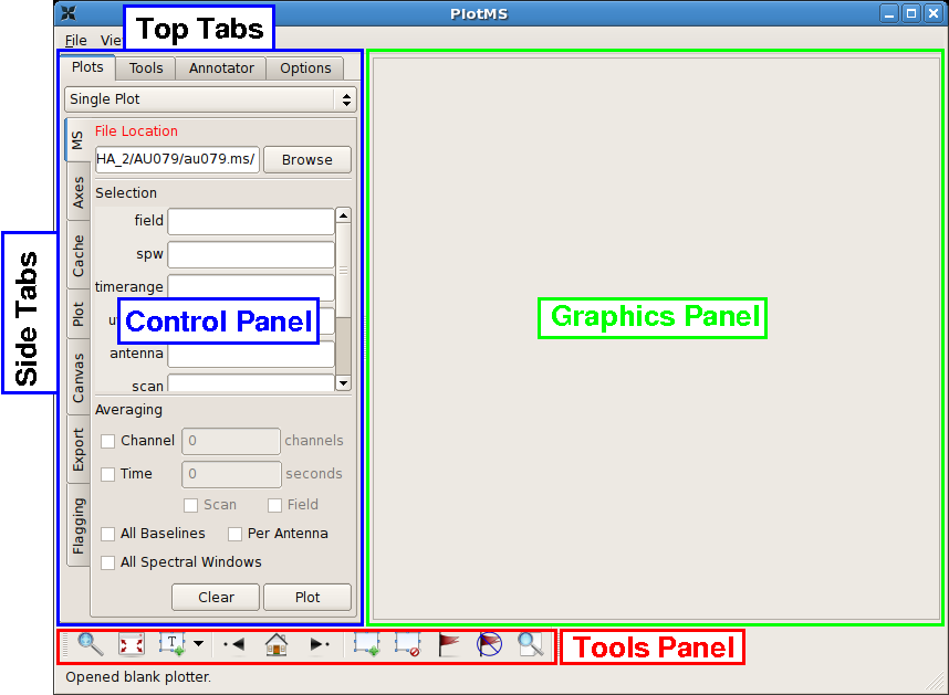
This command brings up the PlotMS window, shown with annotations at right. The window comprises three panels: the control panel (outlined in blue), the graphics panel (green), and the tools panel (red). The control panel controls the selection of data for display and the graphing parameters (axis selection, axis limits, and so on). The graphics panel is the display panel for two-dimensional (x, y) projections of the data. The tools panel provides commands to interact with the graphics panel. The control panel further breaks down into a series of tabs, annotated as Top Tabs and Side Tabs, which contain related plotting and editing control parameters. This tutorial employs only the Plots tab among the Top Tabs and the following Side Tabs.
In this tutorial, interactive commands in the PlotMS window will be summarized as (Tab)Command,, where (Tab) represents the Side Tab where the command is found, and Command is the appropriate GUI interaction (button press, text field, checkbox, etc.). Use the (MS)Browse button, or enter the full pathname, to navigate to and select the measurement set (here, au079.ms).
|
Identifying Bad Data by Discrepant Amplitudes
|
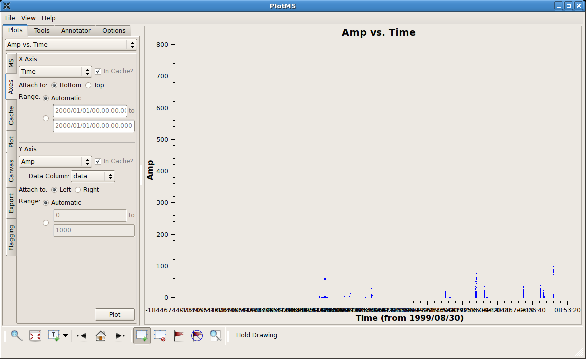
Have a first look at the data by hitting the (MS)Plot button. By default, the axes will be visibility amplitude vs. time. The x-axis labeling is a little garbled in this development version of the software, but straightaway there appear some wildly discrepant data. For a typical decimeter-wave continuum data set, sources and calibrators are expected to show visibility amplitudes of a few Jy or less; visibilities with amplitudes in the 100s of Jy range are |
Examining Individual Sources within a Measurement Set
Antenna-Based Flagging
--Jack Gallimore 14:38, 1 December 2009 (UTC)


