Imaging Flanking Fields: Difference between revisions
| Line 260: | Line 260: | ||
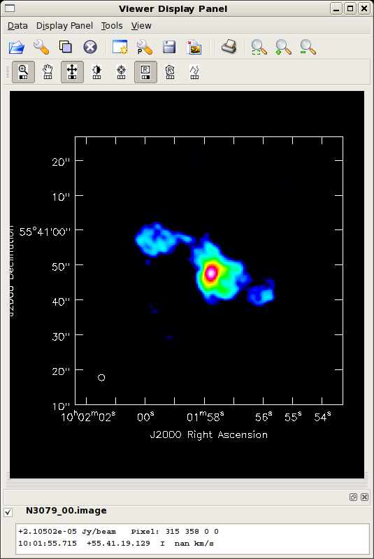
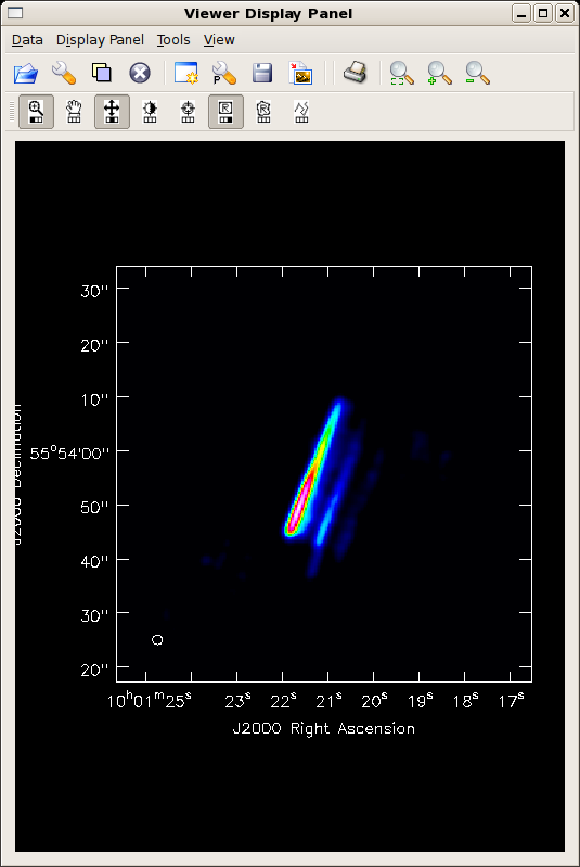
The resulting clean-deconvolved images will be stored in N3079_00.image, N3079_01.image, etc and can be viewed using [[viewer]]. The first two images are shown in the figures above and right. Note that the first flanking field (confusing source) is the famous double QSO [http://www.astr.ua.edu/keel/agn/q0957.html 0957+561]. Because it is located so far from the phase center, the image is distorted, stretched radially from the pointing center of the observation. This sort of distortion is a telltale sign of [http://www.vla.nrao.edu/astro/guides/vlas/current/node16.html bandwidth-smearing]. | The resulting clean-deconvolved images will be stored in N3079_00.image, N3079_01.image, etc and can be viewed using [[viewer]]. The first two images are shown in the figures above and right. Note that the first flanking field (confusing source) is the famous double QSO [http://www.astr.ua.edu/keel/agn/q0957.html 0957+561]. Because it is located so far from the phase center, the image is distorted, stretched radially from the pointing center of the observation. This sort of distortion is a telltale sign of [http://www.vla.nrao.edu/astro/guides/vlas/current/node16.html bandwidth-smearing]. | ||
--[[User:Jgallimo| | --[[User:Jgallimo|Jack Gallimore]] 20:42, 12 November 2009 (UTC) | ||
Revision as of 14:41, 1 December 2009
Overview
The ability to image flanking fields will be introduced in CASA v. 3.0.0. For the purposes of this tutorial, flanking fields are the locations of neighboring radio sources that can contribute significant, confusing signal to your science target. The confusing signal is introduced through sidelobes, which are local maxima of the point response function, or beam, of the array. The contaminating sidelobes are reduced by imaging and deconvolving the neighboring radio sources. AIPS users will recall the task MX which first handled this sort of imaging, later replaced by the AIPS task IMAGR.
One approach is simply to make a sufficiently large image around your science target to include neighboring radio sources, but unfortunately these images can become inconveniently (or impractically) large. There are two angular scales important to the discussion: the synthesized beam and the primary beam. The synthesized beam is the effective angular resolution of the array and is determined by the longest baselines, or telescope separations. The primary beam is a measure of the field-of-view, limited by the angular resolution of a single telescope in the array, which is determined by its physical diameter. The response to radio sources outside 1-2 times the primary beam is very poor, and, unless they are peculiarly bright, such radio sources will contribute negligible confusing signal. The scale of both synthesized beam and the primary beam can be approximated by the Rayleigh criterion.
Here's the problem. Long baseline configurations require small pixels to sample the synthesized beam, and the number of pixels required to map the primary beam becomes inconveniently large. To illustrate, the following table lists the image sizes required to map the VLA primary beam at observing frequency 1.4 GHz and for the four primary array configurations. The primary beam at this frequency is ~32'.
| Configuration | A | B | C | D |
|---|---|---|---|---|
| Synthesized Beam(") | 1.4 | 4.6 | 15 | 50 |
| Pixels | 4200 | 1300 | 380 | 120 |
The upshot is that VLA A-array and B-array observations would require very large, mostly empty images to map the primary beam. It's potentially faster and certainly lighter on disk space to make postage stamp images, or smaller images centered at the science target and flanking fields that contain bright radio sources.
To set up flanking fields in clean, you just need to set up appropriate lists for phase centers, image names, and image sizes. The following is an example specifically from the help file for clean.
# example from the clean help file
imagename = ['M1_0','M1_1','M1_2']
imsize = [
          [1024,1024],
          [128,128],
          [128,128]
         ]
phasecenter = [
               'J2000 13h27m20.98 43d26m28.0',
               'J2000 13h30m52.159 43d23m08.02',
               'J2000 13h24m08.16 43d09m48.0'
              ]
Alternatively, especially if there are many confusing sources, the parameter outlierfile allows clean to read in a list of coordinates and image sizes from a specified text file.
Example: VLA A-array Continuum Observations of NGC 3079
To illustrate the use of flanking fields, this tutorial will demonstrate how to image archival 1.4 GHz, A-array observations of NGC 3079. These data (program AU079) may be obtained from the VLA Archive. NGC 3079 is an edge-on galaxy with kiloparsec-scale, minor-axis radio lobes.
Determining the Location of Flanking Fields
There are two approaches to determining the location of flanking fields. The first is to make a tapered image with large pixels and map the primary beam at artificially poorer angular resolution. The positions of confusing sources can be read off using the CASA viewer. The second approach is to use the on-line NVSS catalog, which has effectively performed the tapering and imaging for you.
This tutorial will outline the NVSS method. The location of flanking fields is determined in two steps: (1) generate an NVSS postage stamp image to identify potential confusing radio sources by eye, and (2) use the NVSS catalog to look up accurate coordinates of the confusing sources.
NVSS Postage Stamp Image Server

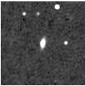
First, use the postage stamp image server to generate an NVSS image of radio sources surrounding NGC 3079. Example inputs to the form are shown in the figure below, and the result is shown in the figure at right.
Alternatively, one could specify "FITS" for the image type, and the coordinates of the confusing sources could be read using a FITS image viewer.
From inspection of the postage stamp image, there are 5 radio sources to be imaged including NGC 3079. We'll use the NVSS catalog to get their coordinates.
NVSS Catalog
Appropriate inputs for the NVSS Catalog Browser are shown in the figure below.
The results of this search are provided in the following table. Sources fainter than 10 mJy were removed, and the results are sorted in order of increasing distance from the search center. The Notes column is based on inspection of the postage stamp image.
| RA(2000) | Dec(2000) | Dist(") | Flux(mJy) | Notes |
|---|---|---|---|---|
| 10 01 57.82 | +55 40 48.5 | <2 | 769.4 | NGC 3079 Nucleus |
| 10 01 58.71 | +55 39 33.3 | 74 | 52.0 | Disk of NGC 3079 |
| 10 01 55.53 | +55 42 04.9 | 80 | 44.0 | Disk of NGC 3079 |
| 10 00 58.93 | +55 40 56.7 | 498 | 56.6 | Nearby radio source |
| 10 02 09.96 | +55 51 26.9 | 648 | 19.7 | Nearby radio source |
| 10 02 45.35 | +55 51 25.2 | 754 | 38.6 | Nearby radio source |
| 10 01 21.07 | +55 53 55.8 | 847 | 551.4 | Nearby radio source |
All of the sources associated with NGC 3079 will comfortably image onto one field; the neighboring sources will require the use of flanking fields.
Editing and Calibration
The following script follows the more detailed tutorial, Calibrating a VLA 5 GHz continuum survey. Some things to note:
- This script employs the python glob command, which generates lists of file names based on wildcard matches.
- Antennas 13 and 26 were misbehaving during the run and are flagged after loading the data.
- If all goes well, the script will generate two measurement sets, "au079.ms," which is the measurement set containing the source and its calibrators, and "N3079.split.ms," which contains the primary calibrated data for N3079.
- It's also worth spending some time interactively editing data with viewer. The tutorial Data flagging with viewer illustrates the procedure specifically for this data set.
# from loaddata.py
from glob import glob

# Define the list of files for reading. Use glob to perform wildcard matching with VLA archive filenames.
fileList = glob('AU079_*.xp?')

importvla(archivefiles=fileList,vis='au079.ms')
listobs('au079.ms')
vishead('au079.ms')

# used viewer to view au079.ms and identified flaky telescopes
# also used casaplotms to identify residual, flaky visibilities

default(flagdata)
vis = 'au079.ms'
# these antennas were producing some junk!
antenna = '10,13'
spw = '0,1'
correlation = ''
timerange = ''
mode = 'manualflag'
clipexpr = 'I'
flagdata()

antenna = ''
mode = ''

# from au079.py
#vis = 'au079.ms'
#xaxis = 'x'
#plotxy()

myRefAnt = 'VA06'
myChans = '0,1'

ampcallist = ['1331+305']
phasecallist = ['0957+553']
sourcelist = ['N3079']
allcals = ampcallist + phasecallist
calDict = {'N3079':'0957+553'}


# set flux calibrator numbers
default(setjy)
modimage = '/usr/lib64/casapy/data/nrao/VLA/CalModels/3C286_L.im'
setjy('au079.ms', field = ampcallist[0], spw=myChans)

# generate initial calibration solutions
rmtables('cal.G')
gaincal(vis='au079.ms',spw=myChans,caltable='cal.G', field=','.join(allcals), solint='inf',
        refant=myRefAnt, append=False, gaincurve=True)

# generate amplitude calibration for phase cal
rmtables('cal.Gflx')
fluxscale(vis='au079.ms', caltable='cal.G',reference=','.join(ampcallist), transfer
          = ','.join(phasecallist), fluxtable='cal.Gflx', append=False)

# apply calibrations to the source
# first, generate a blank table
accum(vis='au079.ms',tablein='',accumtime=10.0,incrtable='cal.Gflx',
      interp='linear', caltable='multisource.gcal',
      field=','.join(allcals), calfield=','.join(allcals))
# now accumulate solutions onto that table
# loop over the source and calibrator pairs in the calDict dictionary variable
for source, calibrator in calDict.iteritems():
    accum(vis='au079.ms',tablein='multisource.gcal',accumtime=10.0,
          incrtable='cal.Gflx',
          interp='linear', field=source,
          calfield=calibrator)
# Finally, apply the calibrations to the measurement set
default(applycal)
applycal(vis='au079.ms', gaintable='multisource.gcal',
         gaincurve=True)

splitfile = 'N3079.split.ms'
rmtables(splitfile) # get rid of any old versions before splitting
split(vis='au079.ms',outputvis=splitfile, datacolumn='corrected', field='N3079', spw=myChans)
Imaging with Flanking Fields


Imaging with flanking fields uses either the outlierfile or phasecenter parameter of clean; in this tutorial we'll use the phasecenter parameter. First, set up clean. The listed parameter choices are reasonable for a VLA snapshot, 1.4 GHz continuum observation.
vis                 =         'N3079.split.ms'
outlierfile         =         ''
field               =         ''
spw                 =         '0,1'
selectdata          =      False
mode                =     'mfs'
gridmode            =         ''
niter               =        5000
gain                =        0.1
threshold           =   '0.04mJy'
psfmode             =    'clark'
imagermode          =         'csclean'
cyclefactor         =         2
cyclespeedup        =         50
multiscale          =         []
interactive         =      False
mask                =         []
cell                = ['0.3arcsec', '0.3arcsec']
restfreq            =         ''
stokes              =        'I'
weighting           =  'natural'
uvtaper             =      False
modelimage          =         ''
restoringbeam       =       ['']
pbcor               =      False
minpb               =        0.1
calready            =       True
async               =      False
Now, set up the flanking fields. For each field, we need an imagename, a phasecenter, and an image size (in pixels).
imagename = [
    'N3079_00',
    'N3079_01',
    'N3079_02',
    'N3079_03',
    'N3079_04'
    ]        #  Pre-name of output images

phasecenter = [
    'J2000 10h01m57.82 +55d40m48.5',
    'J2000 10h01m21.07 +55d53m55.8',
    'J2000 10h00m58.93 +55d40m56.7',
    'J2000 10h02m09.96 +55d51m26.9',
    'J2000 10h02m45.35 +55d51m25.2'
    ]

imsize = [
    [512,512],
    [256,256],
    [256,256],
    [256,256],
    [256,256]
    ]

clean()
The resulting clean-deconvolved images will be stored in N3079_00.image, N3079_01.image, etc and can be viewed using viewer. The first two images are shown in the figures above and right. Note that the first flanking field (confusing source) is the famous double QSO 0957+561. Because it is located so far from the phase center, the image is distorted, stretched radially from the pointing center of the observation. This sort of distortion is a telltale sign of bandwidth-smearing.
--Jack Gallimore 20:42, 12 November 2009 (UTC)

