Sunspot Band6 Imaging for CASA 6.5.4: Difference between revisions
No edit summary |
No edit summary |
||
| Line 1: | Line 1: | ||
[[Category:ALMA]][[Category:Imaging]][[Category:Sun]] | [[Category:ALMA]][[Category:Imaging]][[Category:Sun]] | ||
{{checked_6.5.4}} | |||
==Overview== | ==Overview== | ||
This portion of the | This portion of the guide will cover the image synthesis of a sunspot. It begins where [[Sunspot_Band6_Calibration_for_CASA_6.5.4]] is completed. If you completed the calibration, you may continue working in the directory 'Sunspot_Band6_UncalibratedData'. | ||
If you did not complete the calibration portion of the guide, the calibrated visibility data is available to download at [[Sunspot_Band6#Obtaining the Data]] | |||
Once the download has finished, unpack the file: | Once the download has finished, unpack the file: | ||
<source lang='bash'> | <source lang='bash'> | ||
# | # In bash | ||
tar -xvzf Sunspot_Band6_CalibratedData.tgz | tar -xvzf Sunspot_Band6_CalibratedData.tgz | ||
cd Sunspot_Band6_CalibratedData | cd Sunspot_Band6_CalibratedData | ||
</source> | </source> | ||
==Confirm your version of CASA== | ==Confirm your version of CASA== | ||
This guide has been written for CASA release 6.5. Please confirm your version before proceeding. | This guide has been written for CASA release 6.5. Please confirm your version before proceeding. | ||
<source lang='python'> | <source lang='python'> | ||
# In | # In CASA | ||
from casatools import version | from casatools import version | ||
vernum = str(version()[0])+'.'+str(version()[1]) | vernum = str(version()[0])+'.'+str(version()[1]) | ||
| Line 42: | Line 30: | ||
==Flagging of the surplus scans== | ==Flagging of the surplus scans== | ||
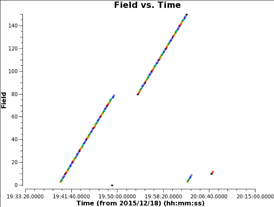
[[File:sunspot_fieldid.png|thumb|right|'''Fig. 1.''' The plot of the FieldID of the scans as a function of the time.]] | [[File:sunspot_fieldid.png|thumb|right|'''Fig. 1.''' The plot of the FieldID of the scans as a function of the time.]] | ||
The actual duration of the observations does not exactly equal to the required duration of the 149-poinitng MOSAIC. Hence, some fields were observed twice, as shown in Figure 1. Although the visibility data of the surplus scans are valid, it is better that they are not used for the image synthesis, considering the uniformity of the sensitivity in a map. For the reason, we flagged the surplus scans by the following command. | |||
<source lang='python'> | <source lang='python'> | ||
# In | # In CASA | ||
msc = ‘uid___A002_Xae00c5_X2a8d_split.ms.cal’ | msc = ‘uid___A002_Xae00c5_X2a8d_split.ms.cal’ | ||
flagdata(vis = msc, mode = 'manual', timerange = '2015/12/18/20:02:35~20:08:20', flagbackup = False) | flagdata(vis = msc, mode = 'manual', timerange = '2015/12/18/20:02:35~20:08:20', flagbackup = False) | ||
| Line 58: | Line 45: | ||
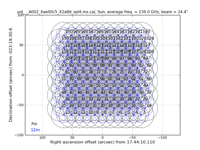
[[File:sunspot_mos2.png|thumb|right|'''Fig. 2.''' The pattern of mosaic AFTER the re-calculation of the direction.]] | [[File:sunspot_mos2.png|thumb|right|'''Fig. 2.''' The pattern of mosaic AFTER the re-calculation of the direction.]] | ||
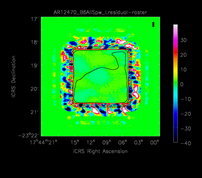
[[File:sunspot_res.png|thumb|right|'''Fig. 3.''' The residual map (color), effective responsibility (black contours) and CLEAN mask (red box).]] | [[File:sunspot_res.png|thumb|right|'''Fig. 3.''' The residual map (color), effective responsibility (black contours) and CLEAN mask (red box).]] | ||
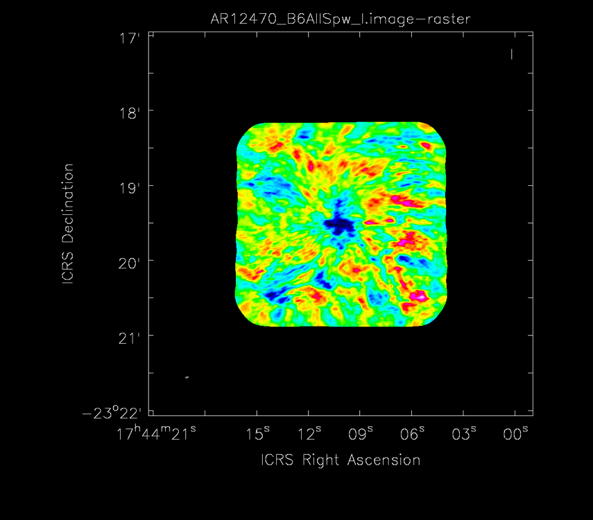
[[File:sunspot_synimg.png|thumb|right|'''Fig. 4.''' The CLEANed image of a sunspot observed with Band6]] | [[File:sunspot_synimg.png|thumb|right|'''Fig. 4.''' The CLEANed image of a sunspot observed with Band6]] | ||
Now we are ready to synthesize a sunspot image from the visibilities. For the image synthesis, we execute the following {{tclean_6.5.4}} command. | |||
<source lang='python'> | <source lang='python'> | ||
# In | # In CASA | ||
tclean(vis = msc, spw = '0,1,2,3', stokes = 'I', field='0,3~150',phasecenter=0, imagename='AR12470_B6AllSpw_I', cell = '0.4 arcsec', imsize = [512, 512], interactive = False, usemask = 'pb', pbmask=0.73, pblimit=0.73, specmode = 'mfs', weighting = 'briggs', robust = 1.0, gridder = 'mosaic', mosweight=True, niter = 100000, deconvolver = 'clark', threshold='1.0Jy', gain=0.1, pbcor=False) | tclean(vis = msc, spw = '0,1,2,3', stokes = 'I', field='0,3~150',phasecenter=0, imagename='AR12470_B6AllSpw_I', cell = '0.4 arcsec', imsize = [512, 512], interactive = False, usemask = 'pb', pbmask=0.73, pblimit=0.73, specmode = 'mfs', weighting = 'briggs', robust = 1.0, gridder = 'mosaic', mosweight=True, niter = 100000, deconvolver = 'clark', threshold='1.0Jy', gain=0.1, pbcor=False) | ||
</source> | </source> | ||
| Line 78: | Line 62: | ||
mask = 'box[[555pix,565pix],[1505pix,1490pix]] | mask = 'box[[555pix,565pix],[1505pix,1490pix]] | ||
</pre> | </pre> | ||
In most cases of solar observations, the field of view (FoV) of the map is filled up with solar structures. Therefore, ideally, the CLEAN box for the solar image synthesis is the same as the FoV. Since the observation was done with the 7m + 12m heterogeneous array, the FoV of the 7m-array is not the same as that of the 12m-array, and the area near the outer edge of the FoV is observed only with 7m-array, as shown in Figure 2. If the CLEAN box includes the area, the synthesized map will include remarkable artificial structures. To avoid the artificial structure, we need to make a CLEAN box that is smaller than the FoV of the 12m-array. In the tutorial, the CLEAN box covers the area that the effective response is larger than 0.73, as shown in Figure 3. | In most cases of solar observations, the field of view (FoV) of the map is filled up with solar structures. Therefore, ideally, the CLEAN box for the solar image synthesis is the same as the FoV. Since the observation was done with the 7m + 12m heterogeneous array, the FoV of the 7m-array is not the same as that of the 12m-array, and the area near the outer edge of the FoV is observed only with 7m-array, as shown in Figure 2. If the CLEAN box includes the area, the synthesized map will include remarkable artificial structures. To avoid the artificial structure, we need to make a CLEAN box that is smaller than the FoV of the 12m-array. In the tutorial, the CLEAN box covers the area that the effective response is larger than 0.73, as shown in Figure 3. | ||
| Line 83: | Line 68: | ||
weighting = 'briggs', robust = 1., | weighting = 'briggs', robust = 1., | ||
</pre> | </pre> | ||
The ‘briggs’ weighting, which is the default weighting option of the CLEAN task, is used for the solar image synthesis. The longest baseline of the 12m-array for the observation is shorter than that of C40-1. However, the visibility data includes the data of over 200m baselines, because the center of the 12m-array is about 200 m distant from the center of the 7m-array. When the robust parameter is set to 0 as a default, the contribution of the longer baseline data is too large and the artificial stripes appear in the synthesized map. For the reason, we set the ‘robust’ value to 1, and the weighting function is set to near the ‘natural’ weighting. The ‘robust’ parameter is not fixed based on the deep optimization. There is still room to examine that. | The ‘briggs’ weighting, which is the default weighting option of the CLEAN task, is used for the solar image synthesis. The longest baseline of the 12m-array for the observation is shorter than that of C40-1. However, the visibility data includes the data of over 200m baselines, because the center of the 12m-array is about 200 m distant from the center of the 7m-array. When the robust parameter is set to 0 as a default, the contribution of the longer baseline data is too large and the artificial stripes appear in the synthesized map. For the reason, we set the ‘robust’ value to 1, and the weighting function is set to near the ‘natural’ weighting. The ‘robust’ parameter is not fixed based on the deep optimization. There is still room to examine that. | ||
| Line 88: | Line 74: | ||
gridder = 'mosaic', mosweight = True | gridder = 'mosaic', mosweight = True | ||
</pre> | </pre> | ||
To deal the data obtain with a heterogeneous array in the CLEAN task, we need to set the ‘mosaic’ option to ‘imagemode’, even when you synthesize an image from the single-pointing data. In most solar cases, the average brightness of a field might be significantly different from that of the other fields. Therefore, we use ‘mosweight’ function. | |||
To deal the data obtain with a heterogeneous array in the CLEAN task, we need to set the ‘mosaic’ option to ‘imagemode’, even when you synthesize an image from the single-pointing data. In most solar cases, the average brightness of a field might be significantly different from that of the other fields. Therefore, we use ‘mosweight’ function. See [[CARMA_spectral_line_mosaic_M99_3.2#Deconvolution_and_Imaging]]. | |||
Figure 4 is the synthesized image from the SV data. | Figure 4 is the synthesized image from the SV data. | ||
| Line 95: | Line 81: | ||
==Primary beam correction and creating of the FITS file== | ==Primary beam correction and creating of the FITS file== | ||
To do the primary beam correction and create the FITS file of the corrected map, the following commands. | To do the primary beam correction and create the FITS file of the corrected map, the following commands. | ||
<source lang='python'> | <source lang='python'> | ||
# In | # In CASA | ||
impbcor(imagename='AR12470_B6AllSpw_I.image', pbimage='AR12470_B6AllSpw_I.pb', outfile='AR12470_B6AllSpw_I.pbcor', mode='divide') | impbcor(imagename='AR12470_B6AllSpw_I.image', pbimage='AR12470_B6AllSpw_I.pb', outfile='AR12470_B6AllSpw_I.pbcor', mode='divide') | ||
exportfits(imagename='AR12470_B6AllSpw_I.pbcor', fitsimage='AR12470_B6AllSpw_I.fits') | exportfits(imagename='AR12470_B6AllSpw_I.pbcor', fitsimage='AR12470_B6AllSpw_I.fits') | ||
Revision as of 18:35, 3 April 2024
Last checked on CASA Version 6.5.4
Overview
This portion of the guide will cover the image synthesis of a sunspot. It begins where Sunspot_Band6_Calibration_for_CASA_6.5.4 is completed. If you completed the calibration, you may continue working in the directory 'Sunspot_Band6_UncalibratedData'.
If you did not complete the calibration portion of the guide, the calibrated visibility data is available to download at Sunspot_Band6#Obtaining the Data Once the download has finished, unpack the file:
# In bash
tar -xvzf Sunspot_Band6_CalibratedData.tgz
cd Sunspot_Band6_CalibratedData
Confirm your version of CASA
This guide has been written for CASA release 6.5. Please confirm your version before proceeding.
# In CASA
from casatools import version
vernum = str(version()[0])+'.'+str(version()[1])
print("You are using CASA ver. "+vernum)
if float(vernum) < 6.5:
 print("YOUR VERSION OF CASA IS TOO OLD FOR THIS GUIDE.")
 print("PLEASE UPDATE IT BEFORE PROCEEDING.")
else:
 print("Your version of CASA is appropriate for this guide.")
Flagging of the surplus scans

The actual duration of the observations does not exactly equal to the required duration of the 149-poinitng MOSAIC. Hence, some fields were observed twice, as shown in Figure 1. Although the visibility data of the surplus scans are valid, it is better that they are not used for the image synthesis, considering the uniformity of the sensitivity in a map. For the reason, we flagged the surplus scans by the following command.
# In CASA
msc = ‘uid___A002_Xae00c5_X2a8d_split.ms.cal’
flagdata(vis = msc, mode = 'manual', timerange = '2015/12/18/20:02:35~20:08:20', flagbackup = False)
flagdata(vis = msc, mode = 'manual', antenna='CM*&DV*;CM*&DA*, flagbackup = False)
Continuum imaging


Now we are ready to synthesize a sunspot image from the visibilities. For the image synthesis, we execute the following tclean command.
# In CASA
tclean(vis = msc, spw = '0,1,2,3', stokes = 'I', field='0,3~150',phasecenter=0, imagename='AR12470_B6AllSpw_I', cell = '0.4 arcsec', imsize = [512, 512], interactive = False, usemask = 'pb', pbmask=0.73, pblimit=0.73, specmode = 'mfs', weighting = 'briggs', robust = 1.0, gridder = 'mosaic', mosweight=True, niter = 100000, deconvolver = 'clark', threshold='1.0Jy', gain=0.1, pbcor=False)
To obtain good SNR of the image, we synthesize an image from the data of all spectrum windows. From here, we will comment only about the options that are the special measures for solar image synthesis.
usemask = 'pb', pbmask = 0.73, pblimit=0.73

mask = 'box[[555pix,565pix],[1505pix,1490pix]]
In most cases of solar observations, the field of view (FoV) of the map is filled up with solar structures. Therefore, ideally, the CLEAN box for the solar image synthesis is the same as the FoV. Since the observation was done with the 7m + 12m heterogeneous array, the FoV of the 7m-array is not the same as that of the 12m-array, and the area near the outer edge of the FoV is observed only with 7m-array, as shown in Figure 2. If the CLEAN box includes the area, the synthesized map will include remarkable artificial structures. To avoid the artificial structure, we need to make a CLEAN box that is smaller than the FoV of the 12m-array. In the tutorial, the CLEAN box covers the area that the effective response is larger than 0.73, as shown in Figure 3.
weighting = 'briggs', robust = 1.,
The ‘briggs’ weighting, which is the default weighting option of the CLEAN task, is used for the solar image synthesis. The longest baseline of the 12m-array for the observation is shorter than that of C40-1. However, the visibility data includes the data of over 200m baselines, because the center of the 12m-array is about 200 m distant from the center of the 7m-array. When the robust parameter is set to 0 as a default, the contribution of the longer baseline data is too large and the artificial stripes appear in the synthesized map. For the reason, we set the ‘robust’ value to 1, and the weighting function is set to near the ‘natural’ weighting. The ‘robust’ parameter is not fixed based on the deep optimization. There is still room to examine that.
gridder = 'mosaic', mosweight = True
To deal the data obtain with a heterogeneous array in the CLEAN task, we need to set the ‘mosaic’ option to ‘imagemode’, even when you synthesize an image from the single-pointing data. In most solar cases, the average brightness of a field might be significantly different from that of the other fields. Therefore, we use ‘mosweight’ function. See CARMA_spectral_line_mosaic_M99_3.2#Deconvolution_and_Imaging.
Figure 4 is the synthesized image from the SV data.
Primary beam correction and creating of the FITS file
To do the primary beam correction and create the FITS file of the corrected map, the following commands.
# In CASA
impbcor(imagename='AR12470_B6AllSpw_I.image', pbimage='AR12470_B6AllSpw_I.pb', outfile='AR12470_B6AllSpw_I.pbcor', mode='divide')
exportfits(imagename='AR12470_B6AllSpw_I.pbcor', fitsimage='AR12470_B6AllSpw_I.fits')
Note: The FITS file can be imported to the data-analysis environment based on SolarSoftWare (SSW) + IDL without any modification, but the coordinate system is the RA/Dec coordinate. You have to convert the coordinate from the RA/Dec coordinate system to the heliocentric coordinate system (X-cen/Y-cen) for the co-alignment with the other solar instrument’s data.