MRK 6: red-shifted HI absorption 6.5.2: Difference between revisions

Revision as of 20:17, 25 January 2023

Last checked on CASA Version 6.5.2

Disclaimer: Due to continuous CASA software updates, GUI images may look different on more recent versions than those shown here.

Overview

This example demonstrates a trickier spectral line data set. In this case, several radio bright active galaxies were observed to look for redshifted 21 cm absorption. The data were obtained using 4IF mode, which means that the full range of velocities were split into two spectral windows (in this example, CASA identifies them as spectral windows 10 and 11). Producing the data cube will require eventually stitching these windows back together. Happily, tclean includes flexible regridding and interpolation in the spectral domain. tclean further allows you to adjust the velocity reference frame.

Retrieve the data from the NRAO archive

Download your data from the VLA Archive; in this example we'll use the publicly available survey AB658 observed in 1992. These data were published in Gallimore et al. (1999).

With the present archive defaults, you should have obtained the following VLA archive file:

'AB658_1_48948.07214_48948.73140.exp'

This tutorial broadly follows the techniques described in the continuum survey tutorial and the 21 cm emission tutorial, and the basic calibration steps are presented only in outline.

Loading the Data

# In CASA
# Import the archive file into a CASA Measurement Set (MS).  
importvla(archivefiles='AB658_1_48948.07214_48948.73140.exp', vis='ab658.ms')

We will now generate a text file listing of the details for the observations using the listobs.

# In CASA
# generate a listobs file with information about the observations as well as printing some details to the terminal
listobs(vis='ab658.ms', listfile='ab658.listobs')

Next we will generate a plot of antenna positions. This will help identify a good reference antenna.

# In CASA
# plot antenna positions
plotants(vis='ab658.ms', figfile='ab658_plotants.png')

For the purposes of this tutorial, we are interested only in the source Markarian 6, but the reduction techniques could be applied to any of the sources in the measurement set.

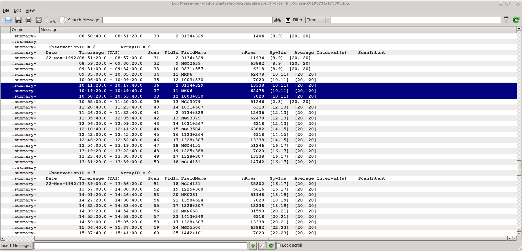
listobs output for AB658. The data for MKN 6 and its calibrators are highlighted.

Using listobs and plotants we learn the source names, spectral windows, and viable reference antennas. A screenshot of the listobs output is given at right.

Source	MKN6
Flux Density Scale Cal	0134+329 = 3C48
Complex Gain Cal	1003+830
Central Antennas	VA27, VA09, VA23
Spectral Window IDs	10, 11

The selection of the spectral windows is key to getting the calibration right. Each science target in the multisource measurement set has a tuning respective of the source redshift, and the calibration observations are matched to those spectral windows. Were the spectral windows parameter (usually spw) left to its default value (all available spectral windows), many calibration routines would necessarily fail.

Editing the Data

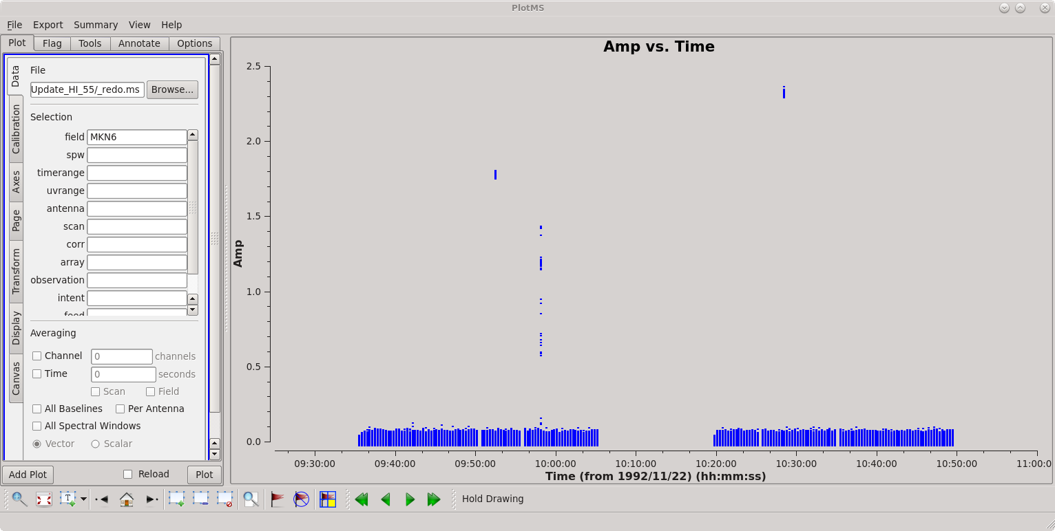
Plotms display of (uncalibrated) visibility amplitudes vs. time for the source MKN 6.

First inspect the data using plotms.

# In CASA
plotms(vis='ab658.ms', field='MKN6', xaxis='time', yaxis='amp')

There is some obvious bad data isolated in time during the observation; see the screenshot at right. We can use the locate tool in plotms to identify specific time ranges or antennas that are causing the problems and flag the bad data with the CASA task flagdata. For more information about flagging data in general, please see our Topical Guide: Flagging VLA Data. Hopefully you find three time ranges that are bad, which will require three calls to flagdata to flag the bad baselines.

# in CASA
flagdata(vis='ab658.ms',antenna='9&12', spw='10', timerange='1992/11/22/09:52:30.00')
flagdata(vis='ab658.ms',antenna='8&18', timerange='1992/11/22/09:58:10.00', spw='10')
flagdata(vis='ab658.ms',antenna='8&9', timerange='1992/11/22/10:28:30.00', spw='10')

Replot the data to confirm flagging has done what is expected.

Calibration

Calibration of HI absorption spectra follows the basic techniques outlined in the continuum tutorial and HI emission tutorial.

First, set the flux denisty of the flux density scale calibrator. Notice that we are being careful to keep track of the spectral windows and not using the default spw.

# In CASA
# set the flux denisty scale standard
setjy(vis='ab658.ms', field='0134+329', spw='10,11', modimage='')

Bandpass calibration comes next.

# In CASA
# bandpass calibration
bandpass(vis='ab658.ms', spw='10,11', caltable='ab658.bcal', gaintable='', gainfield='', interp='', field='0134+329', selectdata=False, bandtype='B', solint='inf', combine='scan', refant='VA27')

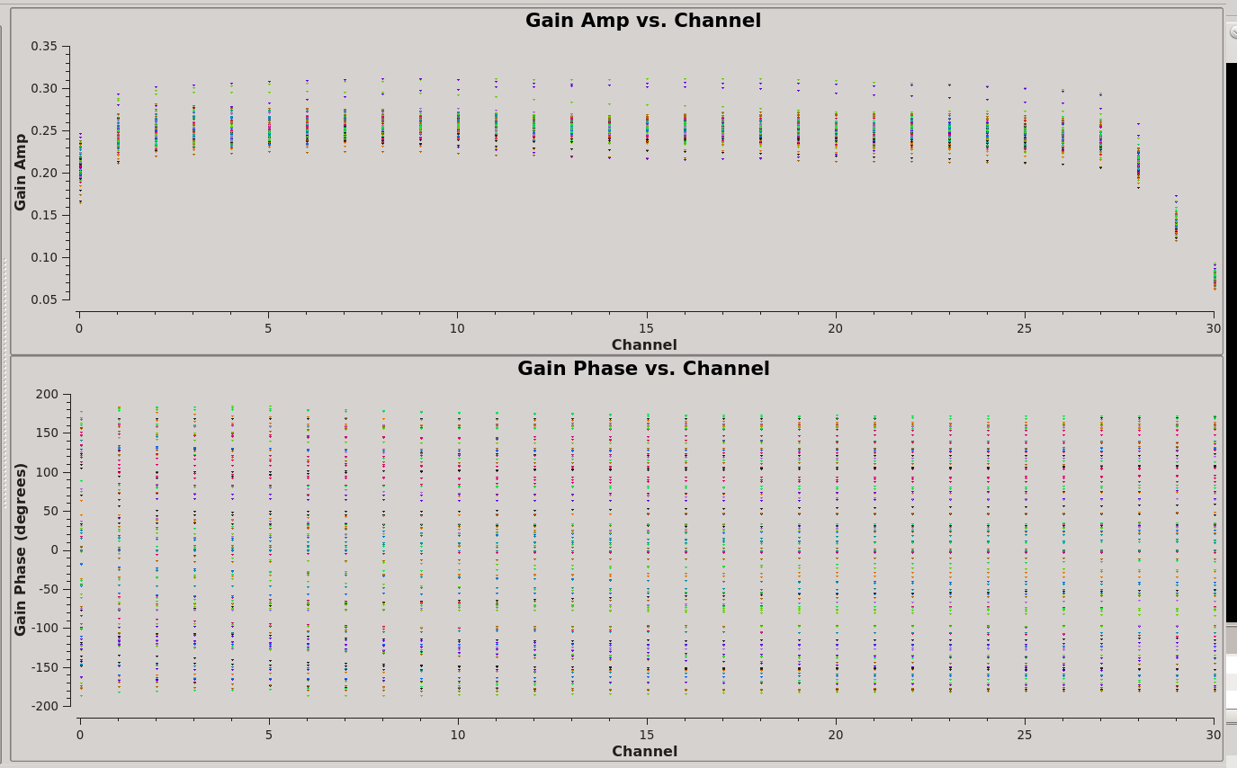
Bandpass calibration curves. Note that the response curve is flat between channels 2 and 27.

In order to perform the flux density scale and complex gain calibrations, we'll need to inspect the bandpass response curve to select appropriate channels to average. We want to choose those channels where the response is relatively flat. The result of plotms is shown at right: the bandpass is flat over channels 2:27.

# In CASA
%cpaste

# Press Enter or Return, then copy/paste all of the following:
# plot the bandpass calibration, amp vs channel
plotms(vis='ab658.bcal', spw='10~11', field='0134+329', gridrows=2, gridcols=1, rowindex=0, plotindex=0, yaxis='gainamp', xaxis='channel', coloraxis='Antenna1')

# plot the bandpass calibration, gain phase vs channel
plotms(vis='ab658.bcal', spw='10~11', field='0134+329', gridrows=2, gridcols=1, rowindex=1, plotindex=1, yaxis='gainphase', xaxis='channel', coloraxis='Antenna1', clearplots=False)
--

The following steps generate amplitude and complex gain solutions for the calibrators, and the fluxscale is bootstrapped from the flux density scale calibrator onto the complex gain calibrator, effectively turning the complex gain calibrator into a local flux density scale calibrator for the science target.

# In CASA
# generate amplitude and gain solutions for complex gain and flux density scale calibrators
gaincal(vis='ab658.ms', caltable='ab658.gcal', gaintable='ab658.bcal', gainfield='', interp='nearest', field='0134+329, 1003+830', 
        spw='10:2~27, 11:2~27', selectdata=False, gaintype='G', solint='inf', combine='', calmode='ap', minsnr=1.0, refant='VA27')

# In CASA
# Bootstrap flux density scale
fluxscale(vis='ab658.ms', fluxtable='MKN6.fluxscale', caltable='ab658.gcal', reference='0134+329', transfer='1003+830')

The task fluxscale will give the bootstrapped flux density of the complex gain calibrator. If all goes well, something like the following should appear in the log window.

Beginning fluxscale--(MSSelection version)-------
 Found reference field(s): 0134+329
 Found transfer field(s):  1003+830
 ...
 Flux density for 1003+830 in SpW=10 (freq=1.3921e+09 Hz) is: 0.492452 +/- 0.00331148 (SNR = 148.711, N = 52)
 Flux density for 1003+830 in SpW=11 (freq=1.39425e+09 Hz) is: 0.489206 +/- 0.00287348 (SNR = 170.249, N = 52)
 ...
 Storing result in ab658.fluxscale

We should inspect the calibration solutions to make sure they are reasonable, but we'll be cavalier and tread forward. Apply the calibrations to the science target and split that target into its own measurement set.

# In CASA
# apply calibrations to science target
applycal(vis='ab658.ms', gaintable=['MKN6.fluxscale','ab658.bcal'], gainfield=['1003+830', '*'], interp=['linear','nearest'], field='MKN6', spw='10,11', spwmap=[], selectdata=False)

#In CASA
# split out the corrected data column (which is placed in the data column in the new MS) for our science target.
split(vis='ab658.ms', outputvis='ab658-MKN6.split.ms', field='MKN6', spw='10:2~27, 11:2~27', datacolumn='corrected')

spw='10:2~27, 11:2~27 : Note that we have selected only the inner channels, 2 through 27 for spectral windows 10, 11.

Continuum Subtraction

Ideally, we would use plotms to identify the channels where HI absorption is present (see the HI emission tutorial.) The absorption line is however weak and isolated against one of a number of radio continuum sources in the data; as such, the absorption is not apparent in averaged visibilities. Instead, we'll have to produce a dirty cube using tclean and inspect the spectrum in the image domain.

Search for the Absorption Line

uvcontsub currently identifies continuum ranges by channel rather than frequency or velocity. We'll make two cubes, one for each spectral window. Note that the act of using split re-indexes the spectral windows and channels. Therefore spw='2~27' have been reindexed and are now spw='0~25' for both channels 10 & 11 (now reindexed as channels 0 & 1).

# In CASA
# image cube for spectral window 0
tclean(vis='ab658-MKN6.split.ms', imagename='temp0', spw='0:0~25', specmode='cube', interpolation='nearest', niter=2000, 
      cell=['0.4arcsec', '0.4arcsec'], phasecenter='J2000 06h52m12.2 +74d25m37')

# In CASA
# make a new image cube with spectral window 1
tclean(vis='ab658-MKN6.split.ms', imagename='temp1', spw='1:0~25', specmode='cube', interpolation='nearest', niter=2000, 
      cell=['0.4arcsec', '0.4arcsec'], phasecenter='J2000 06h52m12.2 +74d25m37')

It's not ordinarily necessary to give the phase center, but this is a good opportunity to use the regridding capabilities of tclean. The data were originally taken in B1950 coordinates, and the observations followed the good practice of offsetting the pointing center slightly away from the source coordinates. Here, we specify the J2000 coordinates (looked up on NED) and allow tclean to handle the precession and centering that we require.

The output cubes will go to temp0.image and temp1.image.

Now we can inspect the cube in viewer.

# In CASA
viewer(infile='temp0.image', displaytype='raster')

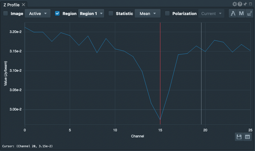
Spectral profile for MKN 6 in the 2nd spectral window, **spw = 1**. The weak absorption line can be seen around channel 15.

Now, use viewer to generate a spectrum. The source spectrum in spw = 1 is shown in the figure at right.

If necessary. use the player buttons to scan through the channels until you see the source.
(Tools)Spectral Profile
Right-click and drag a box around the source; the spectrum will appear in the Image Profile window.
On the Image Profile window, change the velocity convention to Channel using the pull-down menu.
Optional: Save the numerical data to a file. Click the Save button and write the data to a file; for this example, we'll use temp0.txt.

Repeat for spw = 1.

viewer(infile='temp1.image', displaytype='raster')

Perform the Continuum Subtraction

Looking over the plots and text files, only channels 0~25 in either spectral window contain usable data. The absorption line is located in 1:15 and surrounding channels. Just to play it safe, we'll use the channels outside of 1:10~20 (spectral window 1, channels 10-20) to define the continuum for subtraction.

# In CASA
uvcontsub(vis='ab658-MKN6.split.ms', fitspw='0:0~25, 1:0~9; 21~25', solint='int', fitorder=1)

uvcontsub produces the uv subtracted measurement set:

ab658-MKN6.split.ms.contsub (continuum-subtracted visibilities).

Imaging the Continuum Subtracted Cube

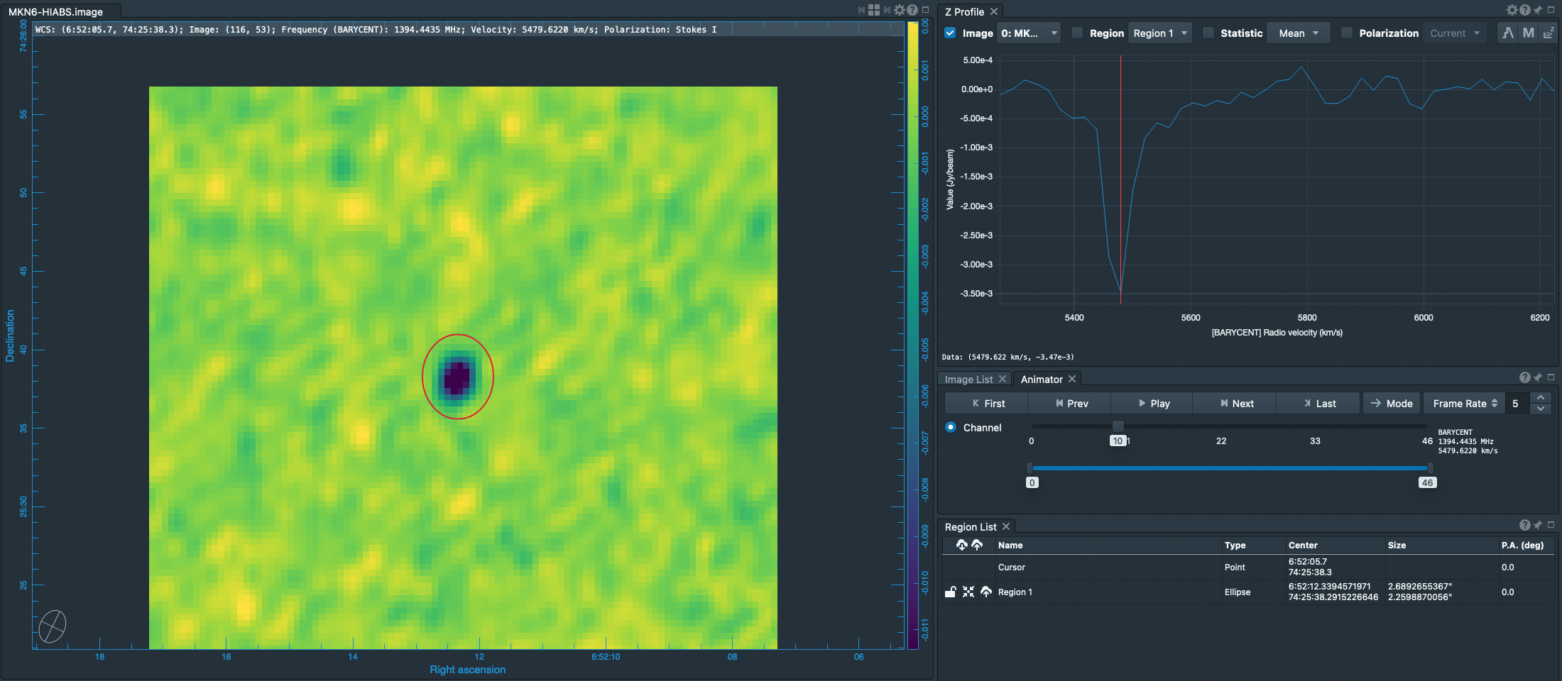
Viewer windows displaying the HI (21cm) absorption line cube of MKN 6. The viewer window shows the channel containing the strongest absorption (at 5479 km/s), and the spectral profile window shows the average spectrum around the position of the strongest absorption.

Inspecting the preliminary (continuum-containing) cubes, temp0.image and temp1.image, that we generated above, we can determine good parameters for the velocity axis.

# In CASA
tclean(vis='ab658-MKN6.split.ms.contsub', spw='', imagename='MKN6-HIABS', specmode='cube', start='-252.349km/s', interpolation='linear',          
      outframe='BARY', veltype='optical', restfreq='1420.405752MHz', niter=2000, threshold='1.0mJy', weighting='natural', cell=['0.4arcsec', '0.4arcsec'], 
      phasecenter = 'J2000 06h52m12.2 +74d25m37')

threshold='1.0mJy' : avoid over-cleaning since it appears that the channel rms is about 0.5 mJy/beam
cell = ['0.4arcsec', '0.4arcsec'] : VLA-A configuration expects 1.5--2 arcsec beams. 0.4arcsec pixels ensure sampling the beam by better than 3x

The (viewer) results are illustrated in the figure at right.

Imaging the Continuum Dataset

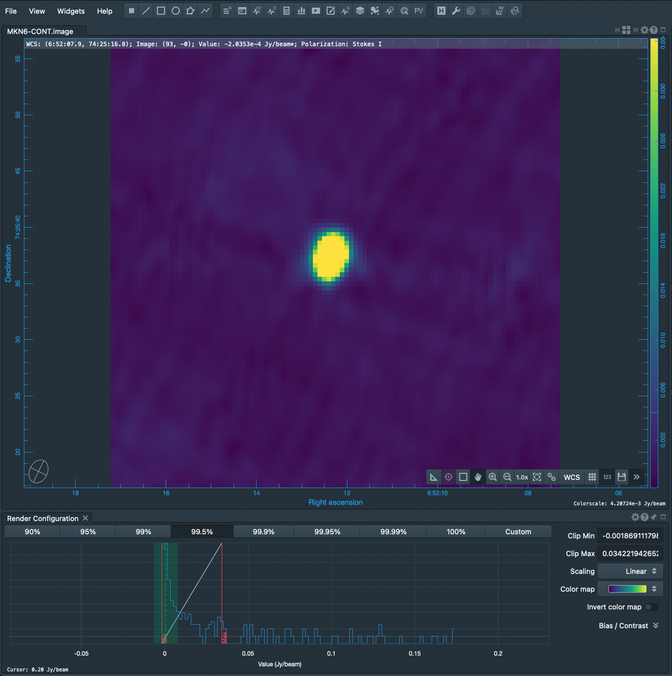
21cm continuum image of MKN 6. The image has been scaled, using (Data)(Adjust)(Basic Settings) **Scaling Power Cycles** = -1.9, to bring out artifacts apparent in the background. The 6-pointed star pattern around the source is symptomatic of residual phase-errors, which can be healed using self-calibration, and the arcuate stripes across the field are sidelobes of neighboring sources that need to be cleaned using flanking fields.

We can similarly image the continuum data with just a few changes of the tclean parameters. Here, we call tclean by selecting the spectral windows and channels pertaining to only the continuum.

# In CASA
tclean(vis='ab658-MKN6.split.ms', specmode='mfs', spw='0:0~25,1:0~9;21~25', imagename='MKN6-CONT', restfreq='1420.405752MHz', niter=2000, 
      threshold='1.0mJy', weighting='natural', cell=['0.4arcsec', '0.4arcsec'], phasecenter = 'J2000 06h52m12.2 +74d25m37')

The result is shown at right. The continuum image needs some more help. Phase errors produce the 6-pointed star pattern surrounding the source and can be healed using self-calibration. The striping across the field is actually the combination of sidelobes from neighboring sources; these sidelobes can be suppressed by cleaning flanking fields.

Extract the Absorption Spectrum

The viewer provides a handy first-look at the spectrum, but the extracted spectrum is an average over a spatial box. What we really want is the integrated spectrum, not the average. To do this, we'll use CASA's imstat, imval, and imhead tools to extract cube information to python variables and then let python build up the spectrum.

Extract the Spectrum: load the cube data into python arrays

First, we need to determine where in the cube to extract the spectrum; equivalently, we need to find the location of the minimum value in the cube. imstat is the tool for this.

# In CASA
cubeStat=imstat("MKN6-HIABS.image")

The variable cubeStat is now a python dictionary. To see what it contains, just enter the variable name:

# In CASA
cubeStat

and the following summary of cubeStat appears.

{'blc': array([0, 0, 0, 0], dtype=int32),
 'blcf': '06:52:17.165, +74.25.16.997, I, 1.39542e+09Hz',
 'max': array([ 0.00286199]),
 'maxpos': array([27, 68,  0,  6], dtype=int32),
 'maxposf': '06:52:14.485, +74.25.44.199, I, 1.39484e+09Hz',
 'mean': array([ -5.30860147e-06]),
 'medabsdevmed': array([ 0.00031676]),
 'median': array([ -3.58635123e-06]),
 'min': array([-0.01634453]),
 'minpos': array([49, 53,  0, 10], dtype=int32),
 'minposf': '06:52:12.299, +74.25.38.200, I, 1.39444e+09Hz',
 'npts': array([ 470000.]),
 'q1': array([-0.00032042]),
 'q3': array([ 0.00031312]),
 'quartile': array([ 0.00063354]),
 'rms': array([ 0.00050688]),
 'sigma': array([ 0.00050685]),
 'sum': array([-2.49504269]),
 'sumsq': array([ 0.12075419]),
 'trc': array([99, 99,  0, 46], dtype=int32),
 'trcf': '06:52:07.331, +74.25.56.597, I, 1.39093e+09Hz'}

These entries can be accessed individually like an array variable. For example, the following commands copy the x and y positions of the absorption line to scalar variables.

# In CASA
%cpaste

# Press Enter or Return, then copy/paste the following:
x2extract = cubeStat['minpos'][0]
y2extract = cubeStat['minpos'][1]
--

Now, extract the spectrum using imval.

# In CASA
%cpaste

# Press Enter or Return, then copy/paste the following:
extractBox = "%d,%d" % (x2extract, y2extract) # copy the position to a string
cubeSpec = imval("MKN6-HIABS.image", box=extractBox, stokes='I')
--

cubeSpec is another python dictionary, and the spectrum is stored in cubeSpec['data'].

Comment: The absorption line source is unresolved by this observation, or, to put it another way, is entirely contained within a synthesized beam. The extraction at a single spatial pixel gives the integrated spectrum and therefore changes units from surface brightness (mJy/beam) to flux density (mJy). However, the data have been forced into a rectangular grid, and there's no guarantee that the absorption minimum centers within a pixel. Better to use imfit to determine more accurately the position of the minimum, and perhaps re-tclean with a new phasecenter. To avoid complicating the present tutorial, we'll just stick with the minimum in the current tclean grid.

Generate the frequency axis

We can derive the frequency axis from the header.

# In CASA
%cpaste

# Press Enter or Return, then copy/paste the following:
import numpy # make sure vector and array arithmetic options are loaded
cubeHead = imhead("MKN6-HIABS.image", mode="list")
nSpec = cubeStat['trc'][3] + 1 # get the number of frequency channels. 
f0 = float(cubeHead['crval4']) # reference freq in Hz
df = float(cubeHead['cdelt4']) # channel width in Hz
i0 = cubeHead['crpix4'] # reference pixel
freqSpec = (numpy.arange(nSpec) - i0)*df + f0
--

Plot the spectrum using matplotlib

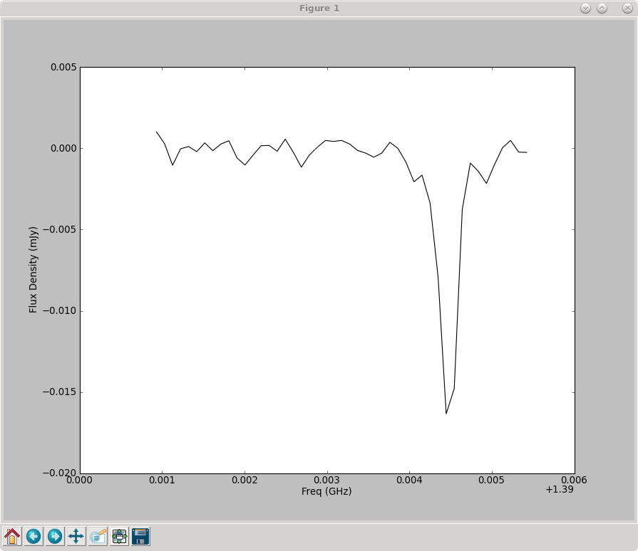
Absorption spectrum of MKN 6 in frequency space.

Now we have the spectrum stored in freqSpec, cubeSpec['data']. Use matplotlib.pyplot to plot the spectrum (see figure at right).

# In CASA
%cpaste


# Press Enter or Return, then copy/paste the following:
import matplotlib.pyplot as plt
plt.clf() # clear the plot (figure)
plt.plot(freqSpec/1.e9, cubeSpec['data'], 'k-')
plt.xlabel("Freq (GHz)")
plt.ylabel("Flux Density (mJy)")
plt.show()
--

A publication-quality figure: plot the spectrum against velocity

Nice, now let's make a velocity axis instead. We'll use the optical convention to convert frequency to velocity; the radio convention is offered as an alternative but is commented out.

# In CASA
%cpaste

# Press Enter or Return, then copy/paste the following:
import matplotlib.pyplot as plt
fRest = cubeHead['restfreq'][0]
velocity = 299792.458 * (fRest/freqSpec - 1.0) # optical convention, km/s
# velocity = 299792.458 * (1.0 - freqSpec/fRest) # radio convention, km/s
--

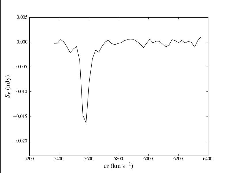
Plot the spectrum again, but this time try for publication-ready quality (see figure at right). This example is somewhat more clever to highlight the use of TeX typography in matplotlib. Note that you will have to have a compatible version of LaTeX installed for this to be successful.

# In CASA
# set up fonts
%cpaste


# Press Enter or Return, then copy/paste the following:
from matplotlib import rc
rc('font',**{'family':'serif','serif':['Times']})
rc('text', usetex=True)
plt.clf() # clear the plot (figure)
plt.plot(velocity, cubeSpec['data'], 'k-')
# the r prefix to the following format strings prevents \ from triggering an escape sequence, 
# like \n for line feed
plt.xlabel(r"$cz$ (km s$^{-1}$)",fontsize=16) 
plt.ylabel(r"$S_{\nu}$ (mJy)",fontsize=16)
plt.ylim(-0.023,0.005)
plt.savefig("mkn6-abs.eps") # save the figure as encapsulated postscript, suitable for journals
plt.savefig("mkn6-abs.png") # save the figure as a bitmap, better suited for astro-ph
--

Save the spectrum to a text file

It's handy to have a simple, columnar text file to inspect and analyze later. Or perhaps you might want to analyze the spectrum outside of CASA. Numpy makes it easy to save and restore text files.

# In CASA
# First, combine the spectrum into a single array
%cpaste

# Press Enter or Return, then copy/paste the following:
spectrum = numpy.vstack((velocity, cubeSpec['data']))
numpy.savetxt("mkn6.txt", numpy.transpose(spectrum))
--

Here's a listing of the first few lines of mkn6.txt.

5.367264765747175261e+03 -2.500247210264205933e-04
5.388621623358961187e+03 -2.288779069203883410e-04
5.409981470534922664e+03  4.886248498223721981e-04
5.431344307902921173e+03  3.546753214322961867e-05
5.452710136090820924e+03 -1.000610413029789925e-03
5.474078955726684399e+03 -2.162145450711250305e-03
5.495450767438905132e+03 -1.413836842402815819e-03
5.516825571855946691e+03 -9.065763442777097225e-04
5.538203369606402703e+03 -3.753502853214740753e-03
5.559584161319202394e+03 -1.479859836399555206e-02

Here's how to restore that text file back into CASA (or python, for that matter).

# In CASA
%cpaste

# Press Enter or Return, then copy/paste the following:
# import numpy # if you haven't already
spectrum = numpy.loadtxt("mkn6.txt",dtype="float")
x = spectrum[:,0]
y = spectrum[:,1]
--

Last checked on CASA Version 5.5.0.