Obtaining EVLA Data: 3C 391 Example

Appendix: Obtaining Data: 3C 391 Example

For the purposes of the summer school tutorials, a small number of initial processing steps had been applied. Here we describe in more detail the series of steps that one is likely to have to conduct to obtain a data set similar to what was used for the summer school tutorials, using the 3C 391 data set as an example.

The original test data were taken on 2010 April 24, and are stored as file TDEM0001_sb1218006_1.55310.33439732639 .

Acquiring data from the Archive

The data are publicly available from the NRAO archive, under Project (Proposal) Name TDEM0001. When submitting an archive query with this project name, the archive lists two separate files; one taken on 2010-Apr-15, and the other on 2010-Apr-24. You will want to download the second file (TDEM0001_sb1218006_1.55310.33439732639; file size 39.79 GB). This file contains data at the full 1-s time resolution. You can select to download an SDM file from the archive, a measurement set, or an AIPS UVFITS file. In the latter two cases, you can opt for spectral or temporal averaging of the data. Spectral averaging prior to bandpass calibration is discouraged, since it can cause phase decorrelation. Whether or not to temporal average will depend on the array configuration, field of view, and acceptable level of time-average smearing. In this example, we opt not to perform any spectral or temporal averaging, and later show how this may be done after the fact by running the task split on the measurement set.

Since the purpose of this tutorial is to demonstrate the steps involved in obtaining one's data from the archive, we will download the data in as unprocessed a format as possible, namely an SDM-BDF dataset (all files). To create a single file (rather than a directory) for downloading, we check the "Create MS or SDM tar file" box, and also check the box labelled "Apply flags generated during observing", to remove data known to be bad (for instance, antennas which are off source during slewing operations).

Having entered your email address at the top of the form and selected the required data set, we now request to "Download checked files". When the data have been copied to the relevant directory, you will receive an email. Follow its instructions to download the tarred SDM file.

Converting to a measurement set

Now that we have the SDM file, untar the file to create a new directory. Then start up CASA, as described in Getting_Started_in_CASA.

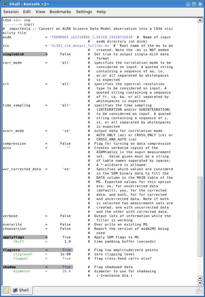
Within CASA, the task importevla will convert a Science Data Model (SDM file) into the Measurement Set (MS) that we will process further using CASA.

# In CASA
importevla(asdm='TDEM0001_sb1218006_1.55310.33439732639',vis='3c391_mosaic_fullres.ms',
   flagzero=True,cliplevel=1e-08,flagpol=True,shadow=True, diameter=28.0)

importevla inputs

While most parameters can be set to their default value, the following should be set explicitly:

• asdm='TDEM0001_sb1218006_1.55310.33439732639' : We must specify the location of the SDM file to be converted.
• vis='3c391_mosaic_fullres.ms' : We must provide a name for the MS to be created.
• flagzero=True : A small fraction of the data is exactly zero, and we wish to get rid of these points, since they are a product of the WIDAR correlator, and do not represent real visibilities. This flagging will proceed via a simple clip, and we must specify the cliplevel, which we set to 1e-08. Anything less than this is unlikely to be real. Since for polarization observations we do not wish to keep the cross-hand visibilities if the parallel hands are zero, we also set flagpol=True.
• shadow=True : When observing at low declinations, particularly in compact configurations, one antenna may block the line of sight between another antenna and the source of interest. This effect is known as shadowing. It is strongly recommended that all data suffering from shadowing be flagged. Knowing the antenna positions, the hour angle and elevation of the source, the shadowing can be computed as a function of antenna and time. By setting the shadow parameter, we opt to flag all shadowed data, regardless of source. To be conservative, we specify diameter=28.0 to set the assumed antenna diameter for calculation of when antennas are shadowed.

This task will take some time to execute, since the SDM file is large (39.79GB) and after creating the MS, it runs flagdata, inspecting every visibility inspected for zeroes and for shadowing.

Averaging the data

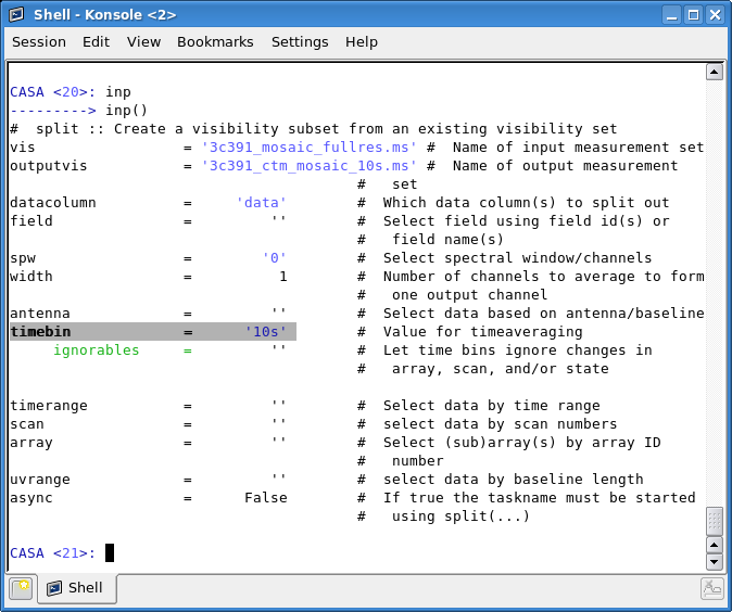
Depending upon the science goals and the details of the observation, averaging in time, frequency, or both may be possible at this stage. For instance, the 3C 391 data used in the summer school tutorial were acquired with a 1-second sampling in the D configuration. Given the size of 3C 391 itself, and the fact that there are no other strong nearby sources, it makes sense to average these data in time (and possibly in frequency as well, although that was not done for the summer school). For the summer school tutorial itself, we also restricted ourselves to just a single spectral window, even though the observations were acquired with two spectral windows. To create a data set averaged in time, we use the task split.

split inputs

split(vis='3c391_mosaic_fullres.ms',outputvis='3c391_ctm_mosaic_10s.ms',datacolumn='data',
      spw='0',width=1,timebin='10s')

This results in a single spectral window, with an unchanged frequency resolution, averaged to 10-second sampling.

• outputvis='3c391_ctm_mosaic_10s.ms' : We specify the name of the new, time-averaged MS.
• datacolumn='data' : In this case, since we have not performed any calibration, we want to take the visibilities from the uncorrected, DATA, column. Were we splitting off the data after calibration, we would instead select the CALIBRATED_DATA column.
• timebin='10s' : Here we specify the time averaging to apply; we write out visibilities averaged to 10s sampling.
• width=1 : This is the number of channels to average to form a single output channel. Here we do no frequency averaging.
• spw='0' : Select only the lower-frequency spectral window (to halve the size of the data set; if you wish to derive spectral index information by using both frequencies, you should set spw= ).

Having created our new 10-s averaged data set, the final step is to create the scratch columns needed in further processing. To do so, we run clearcal. You will recall that we split off the DATA column of the MS. clearcal will then create the MODEL_DATA column (initialized to unity) and the CORRECTED_DATA column (initialized to the values in the DATA column), to remove any previous calibration information and ready the data set for full calibration.

clearcal(vis='3c391_ctm_mosaic_10s.ms')

We have now created the starting data set for the EVLA_Continuum_Tutorial_3C391.