VLA Self-calibration Tutorial-CASA5.7.0: Difference between revisions
| Line 16: | Line 16: | ||
=== Obtaining the Data === | === Obtaining the Data === | ||
The original observation was calibrated using the VLA CASA Pipeline. It can be downloaded from the archive by searching for the SDM name: '''17B-197.sb34290063.eb34589992.58039.86119096065'''. | |||
We will instruct the archive to apply the calibration solutions derived by the original pipeline execution. Therefore, the measurement set (MS) we will be downloading will contain both the raw (uncalibrated) visibilities and the calibrated visibilities, which will appear as the 'DATA' and 'CORRECTED_DATA' columns of the MS, respectively. | |||
The raw data alone is 11.4 GB, and this will become X GB after applying the calibration. | |||
As an alternative to requesting the data from the archive you may instead download the calibrated MS directly here: | |||
-- link to data download -- | |||
=== Observation Details === | === Observation Details === | ||
Revision as of 21:00, 1 July 2019
This page is currently under construction.
Introduction
This CASA guide describes the basics of the self-calibration process and in particular how to choose parameters to achieve the best result. Even after the initial calibration of the dataset using the amplitude calibrator and the phase calibrator, there are likely to be residual phase and/or amplitude errors in the data. Self-calibration is the process of using an existing model, often constructed from imaging the data itself, to reduce the remaining phase and amplitude errors in your image.
The dataset that will be used for this CASA tutorial is an observation of a massive galaxy cluster at z~1 which was taken with the goal to determine the morphology of the radio sources within the cluster.
Data for this Tutorial
Obtaining the Data
The original observation was calibrated using the VLA CASA Pipeline. It can be downloaded from the archive by searching for the SDM name: 17B-197.sb34290063.eb34589992.58039.86119096065.
We will instruct the archive to apply the calibration solutions derived by the original pipeline execution. Therefore, the measurement set (MS) we will be downloading will contain both the raw (uncalibrated) visibilities and the calibrated visibilities, which will appear as the 'DATA' and 'CORRECTED_DATA' columns of the MS, respectively.
The raw data alone is 11.4 GB, and this will become X GB after applying the calibration.
As an alternative to requesting the data from the archive you may instead download the calibrated MS directly here:
-- link to data download --
Observation Details
Once CASA is up and running in the directory containing the data, then start your data reduction by getting some basic information about the data. The task listobs can be used to get a listing of the individual scans comprising the observation, the frequency setup, source list, and antenna locations.
# in CASA
listobs(vis='MOO_1506+5136_Cband.ms')
================================================================================
           MeasurementSet Name:  /filepath/MOO_1506+5136_Cband.ms      MS Version 2
================================================================================
   Observer: Prof. Anthony H. Gonzalez     Project: uid://evla/pdb/34052589
Observation: EVLA(27 antennas)
Data records: 5290272       Total elapsed time = 2853 seconds
   Observed from   13-Oct-2017/20:40:09.0   to   13-Oct-2017/21:27:42.0 (UTC)

Fields: 3
  ID   Code Name                RA               Decl           Epoch   SrcId      nRows
  0    NONE J1549+5038          15:49:17.468534 +50.38.05.78820 J2000   0        1561248
  1    NONE MOO_1506+5136       15:06:20.353700 +51.36.53.63460 J2000   1        3150576
  2    NONE 3C286               13:31:08.287984 +30.30.32.95886 J2000   2         578448
Spectral Windows:  (16 unique spectral windows and 1 unique polarization setups)
  SpwID  Name           #Chans   Frame   Ch0(MHz)  ChanWid(kHz)  TotBW(kHz) CtrFreq(MHz) BBC Num  Corrs
  0      EVLA_C#A0C0#0      64   TOPO    4488.000      2000.000    128000.0   4551.0000       12  RR  RL  LR  LL
  1      EVLA_C#A0C0#1      64   TOPO    4616.000      2000.000    128000.0   4679.0000       12  RR  RL  LR  LL
  2      EVLA_C#A0C0#2      64   TOPO    4744.000      2000.000    128000.0   4807.0000       12  RR  RL  LR  LL
  3      EVLA_C#A0C0#3      64   TOPO    4872.000      2000.000    128000.0   4935.0000       12  RR  RL  LR  LL
  4      EVLA_C#A0C0#4      64   TOPO    5000.000      2000.000    128000.0   5063.0000       12  RR  RL  LR  LL
  5      EVLA_C#A0C0#5      64   TOPO    5128.000      2000.000    128000.0   5191.0000       12  RR  RL  LR  LL
  6      EVLA_C#A0C0#6      64   TOPO    5256.000      2000.000    128000.0   5319.0000       12  RR  RL  LR  LL
  7      EVLA_C#A0C0#7      64   TOPO    5384.000      2000.000    128000.0   5447.0000       12  RR  RL  LR  LL
  8      EVLA_C#B0D0#8      64   TOPO    5488.000      2000.000    128000.0   5551.0000       15  RR  RL  LR  LL
  9      EVLA_C#B0D0#9      64   TOPO    5616.000      2000.000    128000.0   5679.0000       15  RR  RL  LR  LL
  10     EVLA_C#B0D0#10     64   TOPO    5744.000      2000.000    128000.0   5807.0000       15  RR  RL  LR  LL
  11     EVLA_C#B0D0#11     64   TOPO    5872.000      2000.000    128000.0   5935.0000       15  RR  RL  LR  LL
  12     EVLA_C#B0D0#12     64   TOPO    6000.000      2000.000    128000.0   6063.0000       15  RR  RL  LR  LL
  13     EVLA_C#B0D0#13     64   TOPO    6128.000      2000.000    128000.0   6191.0000       15  RR  RL  LR  LL
  14     EVLA_C#B0D0#14     64   TOPO    6256.000      2000.000    128000.0   6319.0000       15  RR  RL  LR  LL
  15     EVLA_C#B0D0#15     64   TOPO    6384.000      2000.000    128000.0   6447.0000       15  RR  RL  LR  LL
Antennas: 27 'name'='station'
   ID=   0-3: 'ea01'='W12', 'ea02'='W04', 'ea03'='W28', 'ea04'='E24',
   ID=   4-7: 'ea05'='E04', 'ea06'='N20', 'ea07'='N16', 'ea08'='W16',
   ID=  8-11: 'ea09'='N12', 'ea10'='E08', 'ea11'='N28', 'ea12'='E28',
   ID= 12-15: 'ea13'='E16', 'ea14'='E36', 'ea15'='N32', 'ea16'='W24',
   ID= 16-19: 'ea17'='N04', 'ea18'='W36', 'ea19'='W20', 'ea20'='N24',
   ID= 20-23: 'ea21'='E20', 'ea22'='W32', 'ea23'='E12', 'ea24'='W08',
   ID= 24-26: 'ea25'='N08', 'ea26'='E32', 'ea27'='N36'
Initial Imaging
First, we want to make an initial image which showcases why we need self-calibration in this case.
We split off the calibrated target field data, meaning that the visibilities of the target source to get copied from the CORRECTED_DATA column to the DATA column of a new measurement set. This is convenient for further processing.
# in CASA
split(vis='MOO_1506+5136_Cband.ms',datacolumn='corrected',field='1',outputvis='obj.ms')
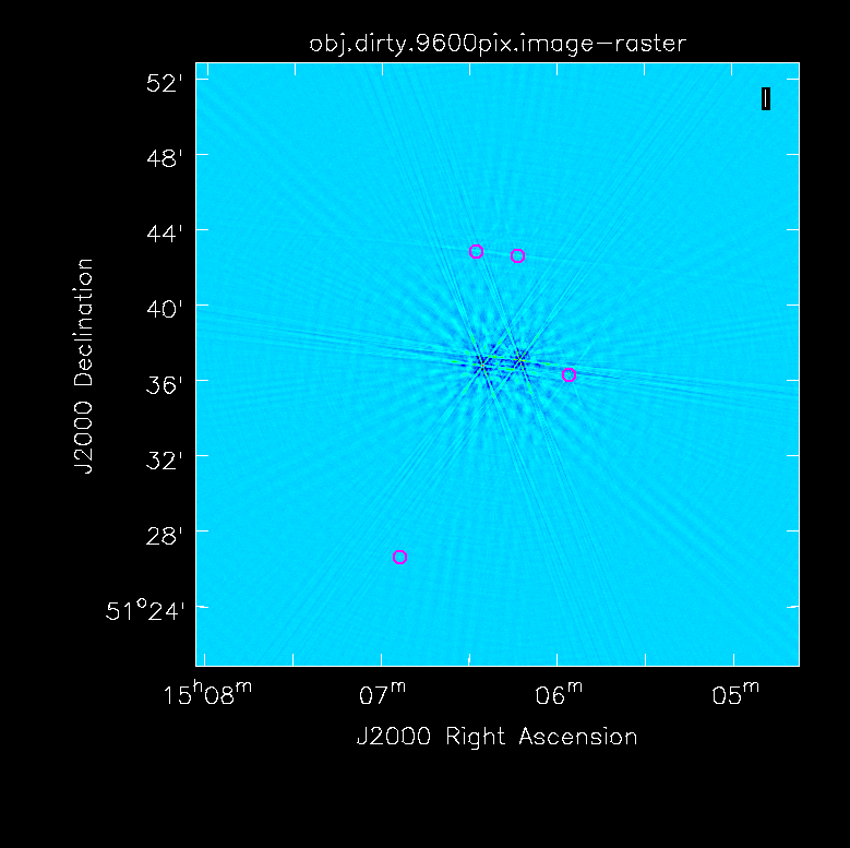
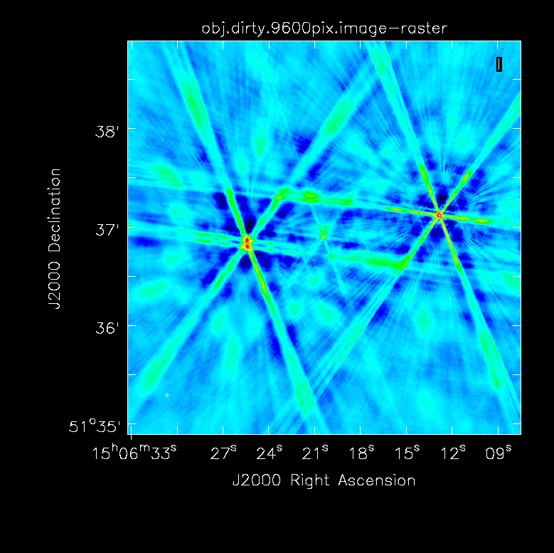
In order to get a feel for the sources in the clusters and any outliers that will need to be cleaned, we make a dirty image of the primary beam.
# in CASA
tclean(vis='obj.ms',imagename='obj.dirty.2000pix.8am.024as',imsize=2000,cell='0.24arcsec',weighting='briggs',niter=1,interactive=False)
- cell='0.24arcsec': The observations were taken in C-band in configuration B which gives a resolution of 1.2". Thus to 5 elements across the resolution of 1.2", we require a cell size of 0.24"/pixel.
- imsize=2000: In this case, the primary beam is ~8'. Thus to get an image of the entire PB, we use an imsize of 2000 pixels.
- niter=1: To make a dirty image, we only need one iteration.
- interactive=False: Turn off the interactive feature to make the dirty image.
 |
 |
Now, we can make a preliminary clean image before rounds of self-calibration to use as a reference.
# in CASA
tclean(vis='obj.ms',imagename='obj.prelim_clean.3am',imsize=750,cell='0.24arcsec',weighting='briggs',deconvolver='mtmfs',niter=1000,interactive=True)
- cell='0.24arcsec': The observations were taken in C-band in configuration B which gives a resolution of 1.2". Thus to 5 elements across the resolution of 1.2", we require a cell size of 0.24"/pixel.
- imsize=750: For the science, we are only interested in the sources within ~1.5' of the cluster center. From the dirty image we also know that there are not any particularly problematic outliers in the field nearby, thus we create a 3' image. Thus to get an image of the entire PB, we use an imsize of 750 pixels.
- deconvolver='mtmfs': Josh:I believe you recommended this to be based on the width of the band of observations with respect to the observing frequency -- I don't remember the qualitative guidelines for center_frequency/total_bandwidth. This corrects for the spectral slope when wideband width -- in this case 1.87GHz.
- niter=1000: Set a relatively large number of iterations as a starting point.
- interactive=True: So we can interactively place the mask.
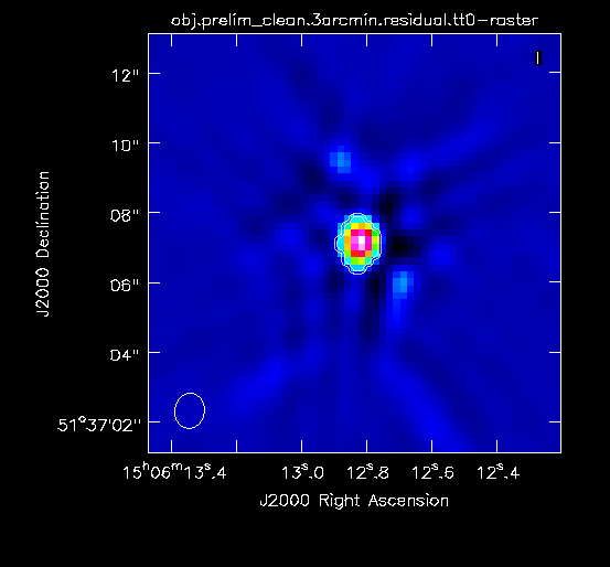
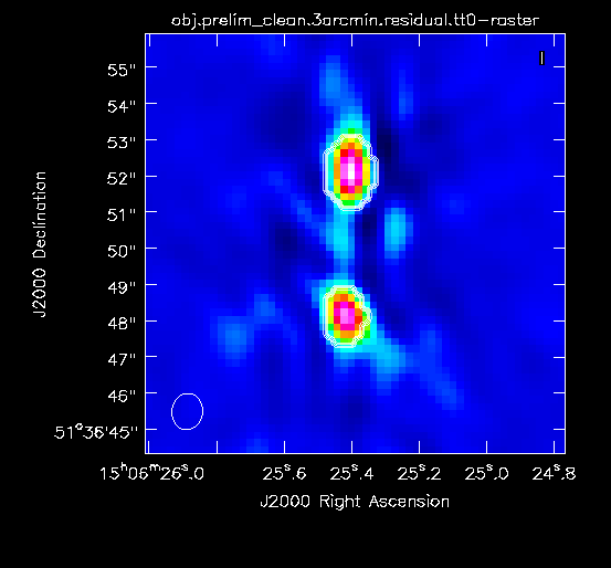
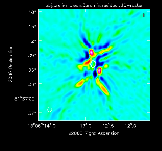
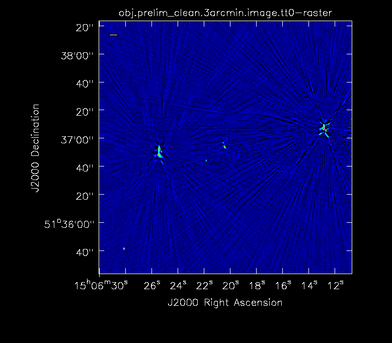
For this preliminary clean, we place circles around each of the strong sources in turn:
- The rightmost source (Figure 2A) -- continue forward and let it clean by pressing the green circle arrow
- The leftmost double-lobed source (Figure 2B)
- The middle source (Figure 2C)
At this point, there is no more emission that is believably real and we stop cleaning (a total of about 225 iterations)(see Figure 2D for an example of the artifacts that are not believable). The final cleaned image without the help of self-cal (Figure 3) shows a lot of artifacts and demonstrates a need for self-calibration (Josh: more details about why need self-cal? or why should we think self-cal would help?).
 |
 |
 |
Self-Calibration Process Outline
What is self-calibration (self-cal)? Self-calibration is the process of using an existing model, often constructed from imaging the data itself, to reduce the remaining phase and amplitude errors in your image. First you create a model using the data itself (using tclean), then iteratively improve this model with further rounds of self-cal (using Template:Gaincall to compare the model to the data and applycal to create a corrected data column).
A few typical cases in which self-cal will help improve the image (Josh: any other ideas?):
- Extensive sidelobes/artifacts from the source of interest or outliers
Each "round" of self-calibration follows a general procedure:
- Conservatively clean target and save the model. Using interactive clean, only include the pixels that you are absolutely certain are real emission as this will be the basis of the model for calibration.
- Use gaincal with a particular solution interval to calculate a table of solutions.
- Check the solutions using plotcal.
- Determine if the solutions should be applied (or if it is time to stop). Is there structure to the solutions?
- Use applycal to apply the table of solutions to the data.
- Use split to make the calibrated data with the applied solutions, the new data (the starting point for the next round of self-cal).
- Start the next round of self-cal.
This guide will cover:
- How to do the self-calibration process in general.
- How to determine optimal selfcal parameters (e.g. solution interval).
- When to stop self-cal.
First Round of Self-Calibration
For this first round of self-cal, we will explore various parameters in order to settle on the optimal parameters. First, we make a conservative clean, meaning that we include in the mask only the pixels that we are absolutely convinced that is real emission.
Preliminary Clean
# in CASA
tclean(vis='obj.ms',imagename='obj.sc_init',imsize=750,cell='0.24arcsec',weighting='briggs',deconvolver='mtmfs',niter=500,savemodel='modelcolumn',interactive=True)
We keep the same parameters as before, but reduce the number of iterations and include savemodel='modelcolumn' which is crucial. By including savemodel, we ensure that the model is explicitly saved to the model column.
Show an example of the masks we used and say approximately how many iterations. It looks like we did just the left source and the middle source. Do you perhaps know why we didn't include the right source at all in the mask? This is perplexing to me as that is the main source that we would want to model I would think.
Check that the model saved?
Choose a Solution Interval
Next, we investigate which solution interval (solint) is optimal for this particular dataset. We will do this by generating and viewing the corrections calculated over several solution intervals (namely on the order of the integration time, 15 seconds, and 45 seconds) using gaincal.
# in CASA
gaincal(vis='obj.ms',caltable='sc1_tb_int',solint='int',refant='ea24',calmode='p',gaintype='T')
- caltable='sc1_tb_int':'Name the calibration tables something intuitive to distinguish each one. In this case, sc1 for self-calibration round 1, tb for table, and int for a solution interval of the integration time.
- solint='int': For this first calibration table, we choose the solutions to be calculated on the level of the integration time (3 seconds in this case) in order to get a sense of the structure and durations of the variations.
- refant='ea24': Choose a reference antenna that is near the center of the array but not the exact center (Josh: I think that is why we chose this one?). In order to view what antennas are near the center use plotants.
- calmode='p': Start with phase only calibration as that is where the most gain is to be had (there is a way more technical way to say that).
- gaintype='T': It is often a good idea to combine the polarizations to understand the overall data.
To view these solutions, we use plotcal.
# in CASA
plotcal(caltable='sc1_tb_int.gain',xaxis='time',yaxis='phase',iteration='antenna',subplot=321)
- xaxis='time' & yaxis='phase': View the phase variations over time with respect to antenna 24.
- iteration='antenna': View the corrections for each antenna.
- subplot=321: It can be helpful to view multiple plots at once, as we will be scrolling through the solutions for each antenna. In this case, 3 rows and two columns.
Show examples of a few of these. gaincal calculates the gains for each antenna/spwid are determined from the ratio of the data column (raw data), divided by the model column, for the specified data selection.(Josh: a bit more about technically what we are looking at and how they affect the data? -- these are the variations in phase between pairs of antennas which can cause the artifacts?) Each color represents a different spectral window. There is definitely structure we want to correct for. We use this solint = int to get a sense of on what time scale the variations occur and the amplitude of the variations. Use the zoom in feature to zoom in on these variations and estimate what the time interval of these variations are. The solint of int shows the variations, but we postulate that a 15 second or 45 second interval would catch these overall variations better.
# in CASA
gaincal(vis='obj.ms',caltable='sc1_tb_15s',solint='15s',refant='ea24',calmode='p',gaintype='T')
gaincal(vis='obj.ms',caltable='sc1_tb_45s',solint='45s',refant='ea24',calmode='p',gaintype='T')
Images of both of these. Comparing the two, we see that they both encapsulate the structure of the variations, however solint=15s encapsulates the variations the best. Thus we choose to apply sc1_tb_15s.gain. Note the amplitude of these variations in sc1_tb_15s.gain; they are typically up to 40 degrees and -60 yo -80 degrees.
Apply Calibration
# in CASA
applycal(vis='obj.ms',gaintable='sc1_tb_15s.gain')
Other potential intervals that could be useful to use are 5 seconds and 60 seconds. Additionally, if the plotcal reveals no structure in these intervals, you can combine the spws together and apply a combined solution by setting combine='spw' (you will have to set spwmap=[0 x number of spectral windows] in apply cal in order to tell CASA to apply the combined solution to all of the spectral windows -- in this case spwmap = [0,0,0,0,0,0,0,0,0,0,0,0,0,0,0,0])
Our goal is to create a better model of the source using the data itself to create a better image. The process with calculating corrections and applying them has (if done correctly) reduced the errors allowing us to make a better image and create a better model. applycal applies the solutions to the (raw) MS DATA column and writes the calibrated data into the CORRECTED_DATA column, thus for determining the next order/level of corrections during the next round of calibration we need to make the corrected data column the data column.
# in CASA
split(vis='obj.ms',outputvis='sc1_obj.ms')
Second Round of Self-Calibration
We will go through the same process again: image, gaincal, applycal, and image. This time the image we create at first will be an indication if the solutions we applied made a difference.
# in CASA
tclean(vis='obj.ms',imagename='obj.sc1',imsize=750,cell='0.24arcsec',weighting='briggs',deconvolver='mtmfs',niter=500,savemodel='modelcolumn',interactive=True)
Larger mask.
# in CASA
gaincal(vis='obj.ms',caltable='sc2_tb_15s',solint='15s',refant='ea24',calmode='p',gaintype='T')
- solint='15s': Since we found a good interval of 15 seconds previously, we move forward with 15s.
Josh: do we want to suggest/show other solution intervals? Do we want to comment on using various intervals -- when is it useful to do several rounds with one interval versus several rounds with each a different solint?
View the solutions.
# in CASA
plotcal(caltable='sc1_tb_int.gain',xaxis='time',yaxis='phase',iteration='antenna',subplot=321)
We can see our corrections made a difference. In particular notice the amplitude of the phase variations, instead of +_60-80 degress they are fractions of a degree. This indicates that we have corrected for a majority of the variations.
When to stop: (looking at amplitude of corrections, image has improved/dynamical range)
Notes about amplitude corrections (?) (mode='ap' or 'a').
When self-cal helped, but didn't improve the image enough: (suggestions for other things to do)