Simulating ngVLA Data-CASA5.4.1: Difference between revisions
No edit summary |
No edit summary |
||
| Line 1: | Line 1: | ||
The following tutorial shows how to | The following tutorial shows how to create simulated data for the next generation Very Large Array (ngVLA). The ngVLA is composed of different subarrays that make up the current reference design. The configuration files for the different subarrays are found in the [http://ngvla.nrao.edu/page/tools "ngVLA Configuration Tools"] and can be used for simulations and calculations that investigate the scientific capabilities of the ngVLA. Each configuration (.cfg) file contains the name of the observatory, the antenna positions, the coordinate system of the antenna positions, and the diameter and the pad name of each antenna. | ||
CASA provides two ways to create a simulation : the {{simobserve}} task and the [https://casa.nrao.edu/docs/CasaRef/simulator-Tool.html#x789-8020002.4.1 ''<tt>sm</tt> toolkit'']. With these methods we can generate measurement sets, add thermal noise and predict model visibilities, from which we can explore the ngVLA’s imaging capabilities. The {{simobserve}} task is very user friendly but it is important to be aware that at the moment it has several limitations when making simulations for observatories other than ALMA and EVLA. For this reason, our suggested method for making simulations, specifically for advanced capabilities, is the <tt>sm</tt> toolkit. The <tt>sm</tt> toolkit provides much more flexibility in the observational parameters and is more compatible with observatories that are not recognized by CASA. | CASA provides two ways to create a simulation : the {{simobserve}} task and the [https://casa.nrao.edu/docs/CasaRef/simulator-Tool.html#x789-8020002.4.1 ''<tt>sm</tt> toolkit'']. With these methods we can generate measurement sets, add thermal noise and predict model visibilities, from which we can explore the ngVLA’s imaging capabilities. The {{simobserve}} task is very user friendly but it is important to be aware that at the moment it has several limitations when making simulations for observatories other than ALMA and EVLA. For this reason, our suggested method for making simulations, specifically for advanced capabilities, is the <tt>sm</tt> toolkit. The <tt>sm</tt> toolkit provides much more flexibility in the observational parameters and is more compatible with observatories that are not recognized by CASA. | ||
In this tutorial | In this tutorial we present three example simulations: (i) simobserve using a model image, (ii) simobserve using a component list, and (iii) a <tt>sm</tt> toolkit simulation. For more information about component lists, see the CASA guides | ||
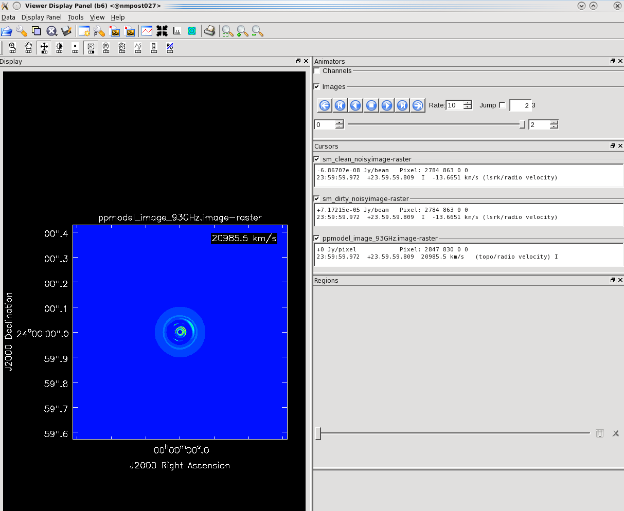
[https://casaguides.nrao.edu/index.php/Simulation_Guide_Component_Lists_(CASA_5.1) "here"] and [https://casaguides.nrao.edu/index.php/Create_a_Component_List_for_Selfcal "here"]. The model image used in portions of this guide can be downloaded [https://casa.nrao.edu/Data/ngVLA/ppmodel_image_3mm.fits.gz " | [https://casaguides.nrao.edu/index.php/Simulation_Guide_Component_Lists_(CASA_5.1) "here"] and [https://casaguides.nrao.edu/index.php/Create_a_Component_List_for_Selfcal "here"]. The model image used in portions of this guide, a 93 GHz model of a protoplanetary disk, can be downloaded [https://casa.nrao.edu/Data/ngVLA/ppmodel_image_3mm.fits.gz "here"]. In this guide, we will create example simulations at 93 GHz of a single channel, observed for a total of 4 hours with a 60 second integration time (in order to keep the measurement set files small). We then add to these simulations an amount of thermal noise that is representative of the ngVLA's continuum sensitivity. The array configuration used in this guide is the Main ngVLA subarray, which is composed of 214 18 m antennas and extends over a maximum baseline of 1005.4 km. The configuration file that we will use through this tutorial is called ngvla-main-revC.cfg and it can be found [http://ngvla.nrao.edu/page/tools "here"]. | ||
=== Estimating the scaling parameter for adding thermal noise === | === Estimating the scaling parameter for adding thermal noise === | ||
Simobserve's parameter to corrupt the simulated data is called '''thermalnoise''' and for interferometric data the allowed values are 'tsys-atm', 'tsys-manual' or False (see more in [https://casaguides.nrao.edu/index.php/Corrupting_Simulated_Data_(Simulator_Tool) "this CASA guide"]). The option 'tsys-atm' is applicable predominantly to ALMA since it uses gain corrections, atmospheric corrections, etc. which are specific to that observatory. | Simobserve's parameter to corrupt the simulated data is called '''thermalnoise''' and for interferometric data the allowed values are 'tsys-atm', 'tsys-manual' or False (see more in [https://casaguides.nrao.edu/index.php/Corrupting_Simulated_Data_(Simulator_Tool) "this CASA guide"]). The option 'tsys-atm' is applicable predominantly to ALMA since it uses gain corrections, atmospheric corrections, etc. which are specific to that observatory. For the option 'tsys-manual', it is necessary to supply several parameters which are required to construct the atmospheric model. In order to achieve the desired sensitivity without atmospheric modeling, we have chosen to corrupt the simulated data using the [https://casa.nrao.edu/docs/CasaRef/simulator.setnoise.html#x822-8350002.4.1 "<tt>sm.setnoise</tt>"] function of the <tt>sm</tt> toolkit. In addition to the modes 'tsys-atm' and 'tsys-manual', this function also allows the option of 'simplenoise'. As the name indicates, 'simplenoise' calculates and adds to the visibilities random Gaussian noise based on a single scaling factor. We will use this same technique for all three example simulations, i.e., those made with the simobserve task and those made with the <tt>sm</tt> toolkit. | ||
In order to estimate the scaling factor for the 'simplenoise' parameter in <tt>sm.setnoise</tt> we use the following procedure: | In order to estimate the scaling factor for the 'simplenoise' parameter in <tt>sm.setnoise</tt> we use the following procedure: | ||
The point source rms noise (<math>\sigma_{NA}</math>) in a Stokes I image | The point source rms noise (<math>\sigma_{NA}</math>) in a Stokes I image will be approximately (see [https://casa.nrao.edu/casadocs/casa-5.4.0/global-tool-list/tool_simulator/methods "<tt>setnoise</tt> function"]) | ||
<math>\sigma_{NA} \sim \frac{\sigma}{ \sqrt{n_{ | <math>\sigma_{NA} \sim \frac{\sigma}{ \sqrt{n_{ch}\,n_{pol}\,n_{baselines}\,n_{integrations} }}</math> (1) | ||
where <math>\sigma</math> is the simplenoise parameter in <tt>sm.setnoise</tt> and corresponds to the noise | where <math>\sigma</math> is the simplenoise parameter in <tt>sm.setnoise</tt> and corresponds to the noise per visibility, <math>n_{ch}</math> is the total number of channels across all spectral windows, <math>n_{pol}</math> is the number of polarizations in the measurement set (typically 2) and <math>n_{integrations}</math> is the number of correlator integration times in the measurement set (i.e., total on-source time / integration time). For this example, the track time is 4 h and the integration time is 60 s, thus <math>n_{integrations}=240</math>. Additionally, the total number of channels is 1. The number of baselines <math>n_{baselines}</math> is estimated by | ||
<math>N(N-1)/2</math> where N is the number of antennas in the array. In this case, N=214 thus <math>n_{baselines}= 22791</math>. | <math>N(N-1)/2</math> where N is the number of antennas in the array. In this case, N=214 thus <math>n_{baselines}= 22791</math>. | ||
Revision as of 16:59, 20 February 2019
The following tutorial shows how to create simulated data for the next generation Very Large Array (ngVLA). The ngVLA is composed of different subarrays that make up the current reference design. The configuration files for the different subarrays are found in the "ngVLA Configuration Tools" and can be used for simulations and calculations that investigate the scientific capabilities of the ngVLA. Each configuration (.cfg) file contains the name of the observatory, the antenna positions, the coordinate system of the antenna positions, and the diameter and the pad name of each antenna.
CASA provides two ways to create a simulation : the simobserve task and the sm toolkit. With these methods we can generate measurement sets, add thermal noise and predict model visibilities, from which we can explore the ngVLA’s imaging capabilities. The simobserve task is very user friendly but it is important to be aware that at the moment it has several limitations when making simulations for observatories other than ALMA and EVLA. For this reason, our suggested method for making simulations, specifically for advanced capabilities, is the sm toolkit. The sm toolkit provides much more flexibility in the observational parameters and is more compatible with observatories that are not recognized by CASA.
In this tutorial we present three example simulations: (i) simobserve using a model image, (ii) simobserve using a component list, and (iii) a sm toolkit simulation. For more information about component lists, see the CASA guides
"here" and "here". The model image used in portions of this guide, a 93 GHz model of a protoplanetary disk, can be downloaded "here". In this guide, we will create example simulations at 93 GHz of a single channel, observed for a total of 4 hours with a 60 second integration time (in order to keep the measurement set files small). We then add to these simulations an amount of thermal noise that is representative of the ngVLA's continuum sensitivity. The array configuration used in this guide is the Main ngVLA subarray, which is composed of 214 18 m antennas and extends over a maximum baseline of 1005.4 km. The configuration file that we will use through this tutorial is called ngvla-main-revC.cfg and it can be found "here".
Estimating the scaling parameter for adding thermal noise
Simobserve's parameter to corrupt the simulated data is called thermalnoise and for interferometric data the allowed values are 'tsys-atm', 'tsys-manual' or False (see more in "this CASA guide"). The option 'tsys-atm' is applicable predominantly to ALMA since it uses gain corrections, atmospheric corrections, etc. which are specific to that observatory. For the option 'tsys-manual', it is necessary to supply several parameters which are required to construct the atmospheric model. In order to achieve the desired sensitivity without atmospheric modeling, we have chosen to corrupt the simulated data using the "sm.setnoise" function of the sm toolkit. In addition to the modes 'tsys-atm' and 'tsys-manual', this function also allows the option of 'simplenoise'. As the name indicates, 'simplenoise' calculates and adds to the visibilities random Gaussian noise based on a single scaling factor. We will use this same technique for all three example simulations, i.e., those made with the simobserve task and those made with the sm toolkit.
In order to estimate the scaling factor for the 'simplenoise' parameter in sm.setnoise we use the following procedure:
The point source rms noise ([math]\displaystyle{ \sigma_{NA} }[/math]) in a Stokes I image will be approximately (see "setnoise function")
[math]\displaystyle{ \sigma_{NA} \sim \frac{\sigma}{ \sqrt{n_{ch}\,n_{pol}\,n_{baselines}\,n_{integrations} }} }[/math] (1)
where [math]\displaystyle{ \sigma }[/math] is the simplenoise parameter in sm.setnoise and corresponds to the noise per visibility, [math]\displaystyle{ n_{ch} }[/math] is the total number of channels across all spectral windows, [math]\displaystyle{ n_{pol} }[/math] is the number of polarizations in the measurement set (typically 2) and [math]\displaystyle{ n_{integrations} }[/math] is the number of correlator integration times in the measurement set (i.e., total on-source time / integration time). For this example, the track time is 4 h and the integration time is 60 s, thus [math]\displaystyle{ n_{integrations}=240 }[/math]. Additionally, the total number of channels is 1. The number of baselines [math]\displaystyle{ n_{baselines} }[/math] is estimated by [math]\displaystyle{ N(N-1)/2 }[/math] where N is the number of antennas in the array. In this case, N=214 thus [math]\displaystyle{ n_{baselines}= 22791 }[/math].
If we know the rms that we want for our resulting image, we can solve for [math]\displaystyle{ \sigma }[/math] which is the scaling parameter of the simplenoise parameter in sm.setnoise.
If instead you want to calculate the expected rms noise for an ngVLA image we suggest the below procedure. This is an example for a simulation at 93 GHz, single channel, 60 s integration time and 4 h of total observation:
(i) Calculate the expected naturally weighted point source sensitivity in a ngVLA performance table. The "ngVLA memo #55 " in Appendix D have key performance metrics for 6 subarrays including the Main interferometric array of the ngVLA where we can find the noise performance values as a function of frequency. For our example, we find in the ngVLA memo #55 Table 10 that the naturally weighted rms at 93 GHz for 1 hour is 0.83 uJy/beam.
(ii) Scale that number to the desired track time, in this case [math]\displaystyle{ t_{track}=4\,h }[/math]. Therefore, [math]\displaystyle{ 0.83/\sqrt{(t_{track}/1\,hour)} = 0.415\,\text{uJy/beam} }[/math].
(iii) Use the desired image noise into the above equation 1 to solve for the simplenoise parameter [math]\displaystyle{ \sigma }[/math]. In this case, [math]\displaystyle{ \sigma=0.415*\sqrt{1*2*240*22791} = 1.4\,\text{mJy} }[/math].
We run sm.setnoise and corrupt the visibilities of the noise-free measurement set using the derived simplenoise parameter [math]\displaystyle{ \sigma }[/math] as follows:
# In CASA
os.system('cp -r noise_free.ms noisy.ms)
sm.openfromms('noisy.ms')
sm.setnoise(mode = ’simplenoise’, simplenoise = sigma)
sm.corrupt()
sm.done()
and your resulting image will have a rms ~ point source noise. Below we present examples of how to make noise-free ms and how to corrupt those visibilities using sm.setnoise.
Simobserve using a model image
We start by making a noise-free ms.
# In CASA
## Using the configuration file obtained from the ngVLA's website
conf_file = 'ngvla-main-revC.cfg'
proj_name = 'ngVLA_214_ant_60s_noise_free'
model_file = 'ppmodel_image_93GHz'

simobserve(project = proj_name,
                    skymodel = model_file+'.fits',
                    inbright = '',
                    incenter = '93GHz',
                    inwidth = '1GHz' ,
                    setpointings = True,
                    integration = '60s',
                    direction = '',
                    mapsize = '',
                    obsmode = 'int',
                    antennalist = conf_file,
                    hourangle = 'transit',
                    totaltime = '14400s',
                    thermalnoise = '',
                    graphics = 'none',
                    overwrite = True)
project: Simobserve will generate a folder with the project name which will contain all the resulting files including the noise-free ms.
skymodel: The input model image in Jy/pixel units. It could be a single image or a spectral cube. The simulated measurement set will inherit the number of channels, central frequency, and peak flux.
incenter: Central frequency of our simulation, in this case is 93 GHz.
inwidth: The bandwidth of the simulation.
%setpointings: allows simobserve to derive the pointing positions by its own algorithm. Given that the primary beam at Q-band is about 1 arcminutes (see the VLA observational status summary (OSS)), and the size of the model is less than an arcsecond, a single pointing will be adequate.
integration: We chose an integration time of 60 s in order to make the simulations faster. Note: An integration time of 60 s is not within the time-smearing limits for the ngVLA Main interferometric array, but for a source in the center of the map it should not be affected by time smearing. However, for future simulations and when considering sources at the edge of the primary beam this value needs to be reconsider and it should be << 0.24 s for this specific subarray.
direction: the center of the map. For a single pointing this is equivalent to the pointing center. Should we specify it?
obsmode: 'int' is used for interferometric data.
antennalist: the ngVLA configuration antenna position file in this case it corresponds to the ngVLA Main interferometric array. The files are available in the "ngVLA's website". Alternatively, the configuration files can be found in CASA in this path: casa.values()[0]['data']+'/alma/simmos/'.
hourangle: is used to simulate observations at a specific hour angle. We use 'transit' for culmination.
totaltime: This is the total track time, in this case the time on source which corresponds to 4 h.
thermalnoise: We leave this parameter empty for this noise-free simulation.
graphics: 'both' will show graphics on the screen such as and save them as png files in the project directory. However, at the moment is not implemented for baselines larger than a few hundred of km. For this reason for our example we use graphics: 'none'.
Now, to add thermal noise we do the following:
# In CASA
## Adding noise with ’simplenoise’
## set the noise level using the simplenoise parameter estimated in section 1
sigma = '1.4mJy'

os.system('cp -r ngVLA_214_ant_60s_noise_free/ngVLA_214_ant_60s_noise_free.ngvla-main-revC.ms ngVLA_214_ant_60s_noisy.ms')
sm.openfromms('ngVLA_214_ant_60s_noisy.ms')
sm.setnoise(mode = 'simplenoise', simplenoise = sigma)
## adds the noise: calculate random Gaussian numbers and add to visibilities
sm.corrupt()
sm.done()
Simobserve using a component list
Instead of using a model image we can generate a component list. Below is a simple example of a Gaussian source.
# In CASA
## Position of the source that we are observing. In this case  the source is in the same location where  the telescope is pointing
direction = me.direction(rf = 'J2000', v0 = qa.unit('00h0m0.0'), v1 = qa.unit('+24.0.0.000'))

## component list cl to make a model centered at the direction given above, and with a source of flux=3.2 Jy
cl.addcomponent(dir = direction, flux = 3.2, freq = '93GHz')

## name of the component list model
cl.rename(filename = 'my_component.cl')

## close the component list
cl.done()
Now, we can run simobserve using the generated component list:
# In CASA
## Using the configuration file obtained from the ngVLA's website
conf_file = 'ngvla-main-revC.cfg'
proj_name = 'ngVLA_214_ant_60s_noise_free'

simobserve(project = proj_name,
                    skymodel = '',
                    complist = 'my_component.cl' ,
                    compwidth = '1GHz',
                    setpointings = True,
                    integration = '60s',
                    direction = '',
                    mapsize = '',
                    obsmode = 'int',
                    antennalist = conf_file,
                    hourangle = 'transit',
                    totaltime = '14400',
                    thermalnoise = '',
                    graphics = 'none',
                    overwrite = True)
And we can add the thermal noise in the same way than in section 2.
sm toolkit using either a model image or a component list
# In CASA
## Using the configuration file obtained from the ngVLA's website
conf_file = 'ngvla-main-revC.cfg'

## If the configuration file is already part of CASA use:
## configdir = casa.values()[0]['data']+'/alma/simmos/'


## Use simutil to read the .cfg file
from simutil import simutil
u = simutil()
xx,yy,zz,diam,padnames,telescope,posobs = u.readantenna(conf_file)
## or use this if the .cfg file is already part of CASA:
## xx,yy,zz,diam,padnames,telescope,posobs = u.readantenna(configdir+conf_file)


##############################################################
## Setting the observation framework  making the resources,
## similar to what we would do in the OPT when setting up
## our observations.
##############################################################

## Simulate measurement set using the simulation utilities sm tool
ms_name = 'ngVLA_214_ant_60s_noise_free.ms'     ## Name of your measurement set
sm.open( ms_name )

## Get the position of the ngVLA using the measures utilities (me)
pos_ngVLA = me.observatory('ngvla')

## set the antenna configuration using the sm tool using the positions,
## diameter and names of the antennas as read from the configuration file
sm.setconfig(telescopename = telescope, x = xx, y = yy, z = zz,
                    dishdiameter = diam.tolist(), mount = 'alt-az',
                    antname = padnames,
                    coordsystem = 'global', referencelocation = pos_ngVLA)


## set the spectral windows, in this case is a single channel
## simulation with a channel resolution of 1 MHz and bandwidth of 1 MHz
sm.setspwindow(spwname = 'Band6', freq = '93GHz', deltafreq = '1MHz',
freqresolution = '1MHz', nchannels = 1, stokes = 'RR RL LR LL')

## set feed parameters for the antennas
sm.setfeed('perfect R L')

## set the field of observation that we are going to simulate
## (where the telescope is pointing), in this example we are using
## a Dec of +24deg
sm.setfield(sourcename = 'My source',
                  sourcedirection = ['J2000','00h0m0.0','+24.0.0.000'])

## set the limit of the observation for the antennas
sm.setlimits(shadowlimit = 0.001, elevationlimit = '8.0deg')

## weight to assign autocorrelation
sm.setauto(autocorrwt = 0.0)

## integration time or how often the array writes one visibility
integrationtime = '60s'
sm.settimes(integrationtime = integrationtime, usehourangle = True,
            referencetime = me.epoch('utc', 'today'))

## setting the observation time, which for our example is 4 h
starttime = '-2h'
stoptime = '2h'
sm.observe('My source', 'Band6', starttime = starttime, stoptime = stoptime)
Now we are going to write a scan of a source using the resource made above. Set the model either using a .fits model or a component list. After that we can predict the visibilities using sm.predict tool function. If using a component list follow the steps below:
## Using the same component list that we generated in section 2
## predicts the visibility of the source
sm.predict( complist = 'my_component.cl')
sm.close()
However, if you want to use a model image instead please follow the steps below:
# In CASA
## To export the .fits file to .image
model_file = 'ppmodel_image_93GHz'
importfits( fitsimage = model_file+'.fits', imagename = model_file+'.image')

## Note: a warning is produced in CASA when running importfits about the image not having a beam or angular resolution. This is expected since the model is in units of Jy/pixel. Please ignore it.

## To predict the model visibilities
sm.predict( imagename = model_file+'.image')

sm.close()
Note: the model image should have units of Jy/pixel and not Jy/beam which in that case will be the restored image.
Finally, in order to add thermal noise we do the following:
# In CASA
## Adding noise with ’simplenoise’
## set the noise level using the simplenoise parameter estimated in section 1
sigma = '1.4mJy'
os.system('cp -r ngVLA_214_ant_60s_noise_free.ms ngVLA_214_ant_60s_noisy.ms')
sm.openfromms('ngVLA_214_ant_60s_noisy.ms')
sm.setnoise(mode = 'simplenoise', simplenoise = sigma)
## adds the noise: calculate random Gaussian numbers and add to visibilities
sm.corrupt()
sm.done()


Last checked on CASA Version 5.4.1.