Protoplanetary Disk Simulation - VLA-CASA5.3.0: Difference between revisions
Created page with " VLA version: under construction!!! Protoplanetary Disk Simulation - VLA Category: Simulations * '''This is an advanced simulation tutorial. New users are recomme..." |
No edit summary |
||
| Line 8: | Line 8: | ||
* '''This is an advanced simulation tutorial. New users are recommended to begin with reading the [http://casa.nrao.edu/casadocs/latest/ CASA Docs] documentation pages on [http://casa.nrao.edu/casadocs/latest/simulation/ "Simulations"].''' | * '''This is an advanced simulation tutorial. New users are recommended to begin with reading the [http://casa.nrao.edu/casadocs/latest/ CASA Docs] documentation pages on [http://casa.nrao.edu/casadocs/latest/simulation/ "Simulations"].''' | ||
* '''This guide is applicable to CASA version 5.1. | * '''This guide is applicable to CASA version 5.1. | ||
* '''To create a script of the Python code on this page see [[Extracting scripts from these tutorials]].''' | * '''To create a script of the Python code on this page see [[Extracting scripts from these tutorials]].''' | ||
== Data == | == Data == | ||
For this CASA Guide we will use a protoplanetary disk model from S. Wolf. Get the data [ | For this CASA Guide we will use a protoplanetary disk model from S. Wolf. Get the data [https://casa.nrao.edu/Data/EVLA/simulation/ppdisk35_GHz_50pc.fits here]. Note that this is a modified image from the [http://casaguides.nrao.edu/index.php?title=Sim_Inputs ALMA Simulation Inputs], where we changed the center frequency 35GHz and the bandwidth to 128MHz. ' | ||
== Script with Explanation == | == Script with Explanation == | ||
| Line 22: | Line 22: | ||
# In CASA | # In CASA | ||
default("simobserve") | default("simobserve") | ||
</source> | |||
Let's call our project "psimvla". This defines the root prefix for any output files from {{simobserve}}. | |||
<source lang="python"> | |||
project = "psimvla" | |||
</source> | </source> | ||
| Line 28: | Line 34: | ||
<source lang="python"> | <source lang="python"> | ||
# This reports image header parameters in the Log Messages window | # This reports image header parameters in the Log Messages window | ||
imhead(" | imhead("ppdisk41_GHz_50pc.fits") | ||
</source> | </source> | ||
This confirms that the data are set at 41GHz center frequency with a bandwidth of 128MHz. Note that the reference coordinate of the image is at pixel (0,0), i.e. in a corner of the image, not the center. In [[https://casaguides.nrao.edu/index.php?title=Protoplanetary_Disk_Simulation_(CASA_5.1)]] a method is provided on how to derive the image centers through the toolkit. Using that method, or inspecting the image with the viewer shows that the image center is at RA=18h00m00.031s, DEC=-22d59m59.6s. | |||
We'll set '''skymodel''' to the FITS file downloaded, above, and leave all '''skymodel''' subparameters at their default values. simobserve will create CASA image <tt> | We'll set '''skymodel''' to the FITS file downloaded, above, and leave all '''skymodel''' subparameters at their default values. {{simobserve}} will create CASA image <tt>psimvla.skymodel</tt>. | ||
<source lang="python"> | <source lang="python"> | ||
skymodel = " | skymodel = "ppdisk41_GHz_50pc.fits" | ||
</source> | </source> | ||
We will specify the sky position for the center of the observation and set the map size to the size of the model image. Since the model image is 2/3 arcseconds across, we should only need one pointing. In this case, '''pointingspacing''' and '''maptype''' can be left at their default values. | We will specify the sky position for the center of the observation and set the map size to the size of the model image. The image is very small compared to the VLA primary beam at 35GHz () Since the model image is 2/3 arcseconds across, we should only need one pointing. In this case, '''pointingspacing''' and '''maptype''' can be left at their default values. | ||
<source lang="python"> | <source lang="python"> | ||
| Line 87: | Line 62: | ||
<source lang="python"> | <source lang="python"> | ||
antennalist = " | antennalist = "vla.a.cfg" | ||
</source> | </source> | ||
| Line 105: | Line 80: | ||
<source lang="python"> | <source lang="python"> | ||
default ("simanalyze") | default ("simanalyze") | ||
project = " | project = "psimvla" | ||
image = True | image = True | ||
</source> | </source> | ||
| Line 112: | Line 87: | ||
<source lang="python"> | <source lang="python"> | ||
modelimage = " | modelimage = "ppdisk41_GHz_50pc.fits" | ||
vis = project + ". | vis = project + ".vla.a.ms" | ||
imsize = [192, 192] | imsize = [192, 192] | ||
</source> | </source> | ||
Revision as of 21:41, 3 May 2018
VLA version: under construction!!!
Protoplanetary Disk Simulation - VLA
- This is an advanced simulation tutorial. New users are recommended to begin with reading the CASA Docs documentation pages on "Simulations".
- This guide is applicable to CASA version 5.1.
- To create a script of the Python code on this page see Extracting scripts from these tutorials.
Data
For this CASA Guide we will use a protoplanetary disk model from S. Wolf. Get the data here. Note that this is a modified image from the ALMA Simulation Inputs, where we changed the center frequency 35GHz and the bandwidth to 128MHz. '
Script with Explanation
Set simobserve as the current task and reset all parameters.
# In CASA
default("simobserve")
Let's call our project "psimvla". This defines the root prefix for any output files from simobserve.
project = "psimvla"
Review the image coordinate system using task imhead.
# This reports image header parameters in the Log Messages window
imhead("ppdisk41_GHz_50pc.fits")
This confirms that the data are set at 41GHz center frequency with a bandwidth of 128MHz. Note that the reference coordinate of the image is at pixel (0,0), i.e. in a corner of the image, not the center. In [[1]] a method is provided on how to derive the image centers through the toolkit. Using that method, or inspecting the image with the viewer shows that the image center is at RA=18h00m00.031s, DEC=-22d59m59.6s.
We'll set skymodel to the FITS file downloaded, above, and leave all skymodel subparameters at their default values. simobserve will create CASA image psimvla.skymodel.
skymodel = "ppdisk41_GHz_50pc.fits"
We will specify the sky position for the center of the observation and set the map size to the size of the model image. The image is very small compared to the VLA primary beam at 35GHz () Since the model image is 2/3 arcseconds across, we should only need one pointing. In this case, pointingspacing and maptype can be left at their default values.
setpointings       =  True
direction          =  "J2000 18h00m00.031s -22d59m59.6s"
mapsize            =  "0.76arcsec"
We do want to simulate an interferometric observation, so we set obsmode accordingly. We'll set totaltime to a 20-minute snapshot observation.
obsmode            =  "int"
totaltime          =  "1200s"
We want to use the appropriate antenna configuration for the desired angular resolution. Configuration 20, alma.out20.cfg, is the largest "compact" configuration. A list of configuration files available in CASA 4.1 is available here.
antennalist = "vla.a.cfg"
We do not want to simulate observations with thermal noise in this example, so we set:
thermalnoise = ''
Now run simobserve.
simobserve()
Now that we've simulated the visibility measurements, we want to generate an image from the simulated data. simanalyze makes this easy. We begin by setting project to the same prefix used in simobserve and setting image to True.
default ("simanalyze")
project = "psimvla"
image = True
We set modelimage to use the input FITS image when cleaning the simulated visibilities. We set the image size to 192 pixels square.
modelimage = "ppdisk41_GHz_50pc.fits"
vis = project + ".vla.a.ms"
imsize = [192, 192]
Specify the number of iterations for cleaning, with proper threshold and weighting.
niter = 10000
threshold = "1e-7Jy"
weighting = "natural"
We'd like to calculate a difference and fidelity image, but we don't need to see the uv coverage.
analyze = True
showuv = False
showresidual = True
showconvolved = True
Plot both to the screen and PNG files with lots of messages.
graphics = "both"
verbose = True
overwrite = True
Run simanalyze.
simanalyze()
Simulation Output
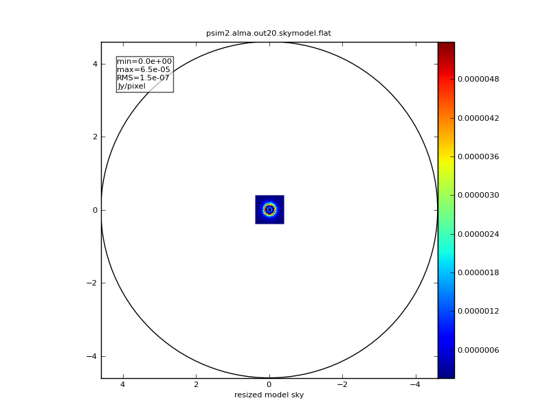
Input:
|
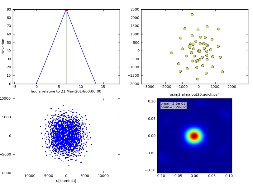
simobserve:
|
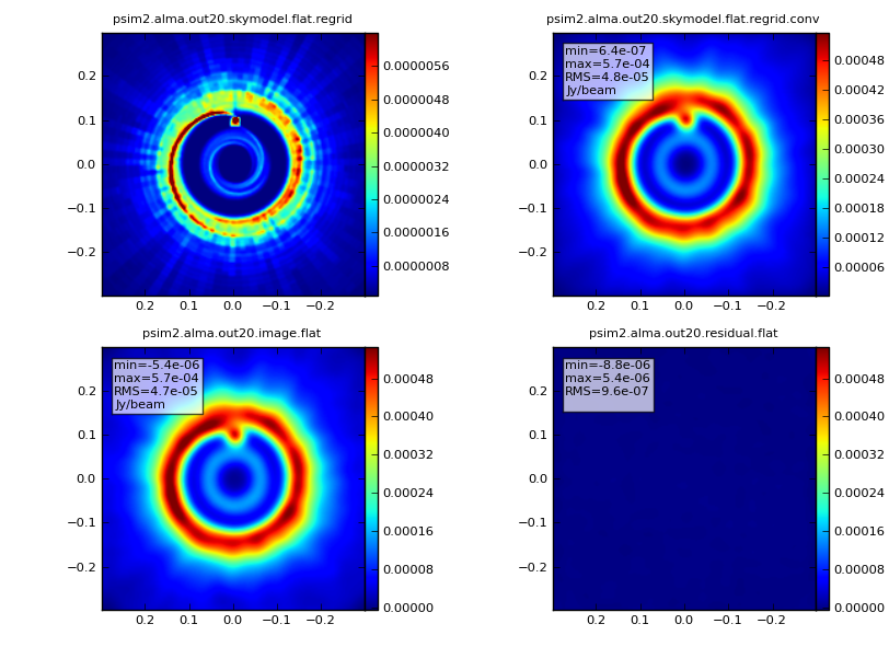
simanalyze image:
|
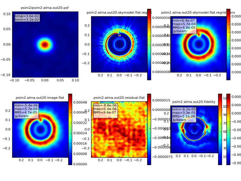
simanalyze output:
|