MRK 6: red-shifted HI absorption 5.5.0: Difference between revisions
No edit summary |
No edit summary |
||
| Line 1: | Line 1: | ||
Disclaimer: Due to continuous CASA software updates, GUI images may look different on more recent versions than those shown here. | Disclaimer: Due to continuous CASA software updates, GUI images may look different on more recent versions than those shown here. | ||
| Line 27: | Line 27: | ||
Recall that the python file globber [http://docs.python.org/library/glob.html glob] is your friend here! | Recall that the python file globber [http://docs.python.org/library/glob.html glob] is your friend here! | ||
Note: IPython's (5.1.0) latest updates prevent copy/pasting several lines of code. To remedy this, we will use the %cpaste command to allow multiple lines to be placed in the terminal. | |||
<source lang="python"> | |||
# In CASA | |||
%cpaste | |||
# Press Enter or Return, then copy/paste the following: | |||
# sort the list of data files and place their names in a list variable | |||
from glob import glob | |||
fileList = sorted(glob("AB658*.xp?")) | |||
# only import if ab658.ms doesn't yet exist, otherwise importvla will throw an error | |||
importvla(archivefiles=fileList, vis='ab658.ms') | |||
-- | |||
</source> | |||
<!-- | |||
<source lang="python"> | <source lang="python"> | ||
| Line 43: | Line 61: | ||
mode = "summary" | mode = "summary" | ||
listobs | listobs | ||
</source> | |||
--> | |||
We will now generate a listing of the details for the observations using the {{listobs}} task. | |||
<source lang="python"> | |||
# generate a listobs file with information about the observations | |||
listobs(vis='ab658.ms', listfile='ab658.listobs') | |||
</source> | |||
Next we will generate a plot of antenna positions. This will help identify a good reference antenna. | |||
<source lang="python"> | |||
# plot antenna positions | |||
plotants(vis="ab658.ms", figfile="ab658_plotants.png") | |||
</source> | </source> | ||
| Line 63: | Line 97: | ||
|} | |} | ||
<!-- | |||
It's just as well to put that information into python global variables. | It's just as well to put that information into python global variables. | ||
| Line 74: | Line 109: | ||
The selection of the spectral windows, stored here in the string variable ''spwStr'', is key to getting the calibration right. Each science target in the multisource measurement set has a tuning respective of the source redshift, and the calibration observations are matched to those spectral windows. Were the spectral windows parameter (usually '''spw''') left to its default value (all available spectral windows), many calibration routines would necessarily fail. | The selection of the spectral windows, stored here in the string variable ''spwStr'', is key to getting the calibration right. Each science target in the multisource measurement set has a tuning respective of the source redshift, and the calibration observations are matched to those spectral windows. Were the spectral windows parameter (usually '''spw''') left to its default value (all available spectral windows), many calibration routines would necessarily fail. | ||
--> | |||
The selection of the spectral windows is key to getting the calibration right. Each science target in the multisource measurement set has a tuning respective of the source redshift, and the calibration observations are matched to those spectral windows. Were the spectral windows parameter (usually '''spw''') left to its default value (all available spectral windows), many calibration routines would necessarily fail. | |||
== Editing the Data == | == Editing the Data == | ||
| Line 81: | Line 120: | ||
First inspect the data using {{plotms}}. | First inspect the data using {{plotms}}. | ||
<source lang="python"> | |||
plotms(vis='ab658.ms', field='MKN6', xaxis='time', yaxis='amp') | |||
</source> | |||
<!-- | |||
<source lang="python"> | <source lang="python"> | ||
plotms(vis = measurementSet, field = sourceName) | plotms(vis = measurementSet, field = sourceName) | ||
</source> | </source> | ||
Be sure to select '''Axes → X Axis → Time''' and '''Axes → Y Axis → Amp'''. There is some obvious junk isolated in time; see the screenshot at right. Follow the [[Data flagging with plotms|tutorial]] to flag discrepant data for the source and calibrators. | |||
Be sure to select '''Axes → X Axis → Time''' and '''Axes → Y Axis → Amp'''. | |||
--> | |||
There is some obvious junk isolated in time; see the screenshot at right. Follow the [[Data flagging with plotms|tutorial]] to flag discrepant data for the source and calibrators. | |||
== Calibration == | == Calibration == | ||
| Line 93: | Line 141: | ||
First, set the flux of the amplitude calibrator. Notice that we are being careful to keep track of the spectral windows and not using the default ''spw''. | First, set the flux of the amplitude calibrator. Notice that we are being careful to keep track of the spectral windows and not using the default ''spw''. | ||
<source lang="python"> | |||
# set the flux standard | |||
setjy(vis='ab658.ms', field='0134+329', spw='10,11', modimage='') | |||
</source> | |||
Bandpass calibration comes next. | |||
<source lang="python"> | |||
# bandpass calibration | |||
bandpass(vis='ab658.ms', spw='10,11', caltable='ab658.bcal', gaintable='', gainfield='', interp='', field='0134+329', selectdata=False, bandtype='B', solint='inf', combine='scan', refant='VA27') | |||
</source> | |||
<!-- | |||
<source lang="python"> | <source lang="python"> | ||
# set the flux standard | # set the flux standard | ||
| Line 134: | Line 195: | ||
bandpass() | bandpass() | ||
</source> | </source> | ||
--> | |||
[[File:MRK6-shot2.png|thumb|Bandpass calibration curves. Note that the response curve is flat between channels 2 and 27.]] | [[File:MRK6-shot2.png|thumb|Bandpass calibration curves. Note that the response curve is flat between channels 2 and 27.]] | ||
| Line 139: | Line 201: | ||
In order to perform the amplitude and phase calibrations, we'll need to inspect the bandpass response curve to select appropriate channels to average. We want to choose those channels where the response is relatively flat. The result of plotcal is shown at right: the bandpass is flat over channels 2:27. | In order to perform the amplitude and phase calibrations, we'll need to inspect the bandpass response curve to select appropriate channels to average. We want to choose those channels where the response is relatively flat. The result of plotcal is shown at right: the bandpass is flat over channels 2:27. | ||
<source lang="python"> | |||
# In CASA | |||
%cpaste | |||
# Press Enter or Return, then copy/paste all of the following: | |||
# plot the bandpass calibration, amp vs channel | |||
plotcal(caltable='ab658.bcal', spw='10,11', field='0134+329', subplot=211, yaxis='amp', showgui=True) | |||
# plot the bandpass calibration, gain phase vs channel | |||
plotcal(caltable='ab658.bcal', spw='10,11', field='0134+329', subplot=212, yaxis='phase', showgui=True) | |||
-- | |||
</source> | |||
<!-- | |||
<source lang="python"> | <source lang="python"> | ||
# plot the bandpass calibration | # plot the bandpass calibration | ||
| Line 153: | Line 229: | ||
plotcal() | plotcal() | ||
</source> | </source> | ||
--> | |||
The following steps generate amplitude and phase solutions for the calibrators, and the fluxscale is bootstrapped from the amplitude calibrator onto the phase calibrator, effectively turning the phase calibrator into a local flux calibrator for the science target. | |||
<source lang="python"> | |||
# generate amplitude and gain solutions for phase and amplitude calibrators | |||
gaincal(vis='ab658.ms', caltable='ab658.gcal', gaintable='ab658.bcal', gainfield='', interp='nearest', field='0134+329, 1003+830', | |||
spw='10:2~27, 11:2~27', selectdata=False, gaintype='G', solint='inf', combine='', calmode='ap', minsnr=1.0, refant='VA27') | |||
</source> | |||
<source lang="python"> | |||
# Bootstrap flux scale | |||
fluxscale(vis='ab658.ms', fluxtable='MKN6.fluxscale', caltable='ab658.gcal', reference='0134+329', transfer='1003+830') | |||
</source> | |||
<!-- | |||
<source lang="python"> | <source lang="python"> | ||
default('gaincal') | default('gaincal') | ||
| Line 188: | Line 276: | ||
fluxscale() | fluxscale() | ||
</source> | </source> | ||
--> | |||
The task {{fluxscale}} will give the bootstrapped flux density of the phase calibrator. If all goes well, something like the following should appear in the log window. | The task {{fluxscale}} will give the bootstrapped flux density of the phase calibrator. If all goes well, something like the following should appear in the log window. | ||
| Line 202: | Line 291: | ||
We should inspect the calibration solutions to make sure they are reasonable, but we'll be [http://en.wikipedia.org/wiki/Virginia_Cavaliers cavalier] and tread forward. Apply the calibrations to the science target and split that target into its own measurement set. | We should inspect the calibration solutions to make sure they are reasonable, but we'll be [http://en.wikipedia.org/wiki/Virginia_Cavaliers cavalier] and tread forward. Apply the calibrations to the science target and split that target into its own measurement set. | ||
<source lang="python"> | |||
# apply calibrations to science target | |||
applycal(vis='ab658.ms', gaintable=['MKN6.fluxscale','ab658.bcal'], gainfield=['1003+830', '*'], interp=['linear','nearest'], field='MKN6', spw='10,11', spwmap=[], selectdata=False) | |||
</source> | |||
<source lang="python"> | |||
# split out the corrected data column (which is placed in the data column in the new MS) for our science target. | |||
split(vis='ab658.ms', outputvis='ab658-MKN6.split.ms', field='MKN6', spw='10:2~27, 11:2~27', datacolumn='corrected') | |||
</source> | |||
* ''spw='10:2~27, 11:2~27'' : Note that we have selected only the inner channels, 2 through 27 for spectral windows 10, 11. | |||
<!-- | |||
<source lang="python"> | <source lang="python"> | ||
default('applycal') | default('applycal') | ||
| Line 229: | Line 331: | ||
split() | split() | ||
</source> | </source> | ||
--> | |||
== Continuum Subtraction == | == Continuum Subtraction == | ||
| Line 236: | Line 339: | ||
=== Search for the Absorption Line === | === Search for the Absorption Line === | ||
{{uvcontsub|Uvcontsub}} currently identifies continuum ranges by channel rather than frequency or velocity. We'll make two cubes, one for each spectral window. | {{uvcontsub|Uvcontsub}} currently identifies continuum ranges by channel rather than frequency or velocity. We'll make two cubes, one for each spectral window. Note that the act of using split re-indexes the spectral windows and channels. Therefore spw='2~27' have been reindexed and are now spw='0~25' for both channels 10 & 11 (now reindexed as channels 0 & 1). | ||
<source lang="python"> | |||
# image cube for spectral window 0 | |||
clean(vis='ab658-MKN6.split.ms', imagename='temp0', spw='0:0~25', mode='channel', nchan=-1, start=0, width=1, interpolation='nearest', niter=2000, | |||
cell=['0.4arcsec', '0.4arcsec'], phasecenter='J2000 06h52m12.2 +74d25m37') | |||
</source> | |||
<source lang="python"> | |||
# make a new image cube with spectral window 1 | |||
clean(vis='ab658-MKN6.split.ms', imagename='temp1', spw='1:0~25', mode='channel', nchan=-1, start=0, width=1, interpolation='nearest', niter=2000, | |||
cell=['0.4arcsec', '0.4arcsec'], phasecenter='J2000 06h52m12.2 +74d25m37') | |||
</source> | |||
<!-- | |||
<source lang="python"> | <source lang="python"> | ||
default(clean) | default(clean) | ||
| Line 257: | Line 373: | ||
clean() | clean() | ||
</source> | </source> | ||
--> | |||
It's not ordinarily necessary to give the phase center, but this is a good opportunity to use the regridding capabilities of {{clean}}. The data were originally taken in B1950 coordinates, and the observations followed the good practice of offsetting the pointing center slightly away from the source coordinates. Here, we specify the J2000 coordinates (looked up on [http://nedwww.ipac.caltech.edu NED]) and allow {{clean}} to handle the precession and centering that we require. | It's not ordinarily necessary to give the phase center, but this is a good opportunity to use the regridding capabilities of {{clean}}. The data were originally taken in B1950 coordinates, and the observations followed the good practice of offsetting the pointing center slightly away from the source coordinates. Here, we specify the J2000 coordinates (looked up on [http://nedwww.ipac.caltech.edu NED]) and allow {{clean}} to handle the precession and centering that we require. | ||
| Line 264: | Line 381: | ||
Now we can inspect the cube in {{viewer}}. | Now we can inspect the cube in {{viewer}}. | ||
<source lang="python"> | |||
viewer(infile='temp0.image', displaytype='raster') | |||
</source> | |||
<!-- | |||
<source lang="python"> | <source lang="python"> | ||
infile = 'temp0.image' | infile = 'temp0.image' | ||
| Line 269: | Line 391: | ||
viewer() | viewer() | ||
</source> | </source> | ||
--> | |||
[[File:MRK6-shot4-annotated.png|thumb|Spectral profile for MRK 6 in the 2nd spectral window, '''spw = 1'''. The location of the weak absorption line is marked by green arrow.]] | [[File:MRK6-shot4-annotated.png|thumb|Spectral profile for MRK 6 in the 2nd spectral window, '''spw = 1'''. The location of the weak absorption line is marked by green arrow.]] | ||
| Line 282: | Line 405: | ||
Repeat for '''spw = 1'''. | Repeat for '''spw = 1'''. | ||
<source lang="python"> | |||
viewer(infile='temp1.image', displaytype='raster') | |||
</source> | |||
<!-- | |||
<source lang="python"> | <source lang="python"> | ||
infile = 'temp1.image' | infile = 'temp1.image' | ||
| Line 287: | Line 415: | ||
viewer() | viewer() | ||
</source> | </source> | ||
--> | |||
=== Perform the Continuum Subtraction === | === Perform the Continuum Subtraction === | ||
| Line 292: | Line 421: | ||
Looking over the plots and text files, only channels 0~25 in either spectral window contain usable data. The absorption line is located in 1:15 and surrounding channels. Just to play it safe, we'll use the channels outside of 1:10~20 (spectral window 1, channels 10-20) to define the continuum for subtraction. | Looking over the plots and text files, only channels 0~25 in either spectral window contain usable data. The absorption line is located in 1:15 and surrounding channels. Just to play it safe, we'll use the channels outside of 1:10~20 (spectral window 1, channels 10-20) to define the continuum for subtraction. | ||
<source lang="python"> | |||
uvcontsub(vis='ab658-MKN6.split.ms', fitspw='0:0~25, 1:0~9; 21~25', solint='int', fitorder=1) | |||
</source> | |||
<!-- | |||
<source lang="python"> | <source lang="python"> | ||
default(uvcontsub) | default(uvcontsub) | ||
| Line 303: | Line 437: | ||
uvcontsub() | uvcontsub() | ||
</source> | </source> | ||
--> | |||
{{uvcontsub|Uvcontsub}} produces the uv subtracted measurement set: | {{uvcontsub|Uvcontsub}} produces the uv subtracted measurement set: | ||
| Line 314: | Line 449: | ||
Inspecting the preliminary (continuum-containing) cubes, temp0.image and temp1.image, that we generated [[#Search for the Absorption Line|above]], we can determine good parameters for the velocity axis. Here are the velocity options I came up with. | Inspecting the preliminary (continuum-containing) cubes, temp0.image and temp1.image, that we generated [[#Search for the Absorption Line|above]], we can determine good parameters for the velocity axis. Here are the velocity options I came up with. | ||
<source lang="python"> | |||
clean(vis='ab658-MKN6.split.ms.contsub', spw='', imagename='MKN6-HIABS', mode='velocity', nchan=-1, start='-252.349km/s', interpolation='linear', width='', | |||
outframe='bary', veltype='optical', restfreq='1420.405752MHz', niter=2000, threshold='1.0mJy', weighting='natural', cell=['0.4arcsec', '0.4arcsec'], | |||
phasecenter = 'J2000 06h52m12.2 +74d25m37') | |||
</source> | |||
* width='' : Set the channel width equal to the first channel in the first spectral window. | |||
* threshold='1.0mJy' : avoid over-cleaning since it appears that the channel rms is about 0.5 mJy/beam | |||
* cell = ['0.4arcsec', '0.4arcsec'] : VLA-A configuration expects 1.5--2 arcsec beams. 0.4arcsec pixels ensure sampling the beam by better than 3x | |||
<!-- | |||
<source lang="python"> | <source lang="python"> | ||
default(clean) | default(clean) | ||
| Line 337: | Line 483: | ||
weighting = 'natural' | weighting = 'natural' | ||
</source> | </source> | ||
Set the source coordinates. We'll use defaults for the rest of the parameters; with the continuum subtracted, the data have only simple structure with no confusing sources. | Set the source coordinates. We'll use defaults for the rest of the parameters; with the continuum subtracted, the data have only simple structure with no confusing sources. | ||
| Line 346: | Line 493: | ||
clean() | clean() | ||
</source> | </source> | ||
--> | |||
The ({{viewer}}) results are illustrated in the figure at upper right. | The ({{viewer}}) results are illustrated in the figure at upper right. | ||
| Line 355: | Line 503: | ||
We can similarly image the continuum data with just a few changes of the {{clean}} parameters. Here, we call clean by selecting the spectral windows and channels pertaining to only the continuum. | We can similarly image the continuum data with just a few changes of the {{clean}} parameters. Here, we call clean by selecting the spectral windows and channels pertaining to only the continuum. | ||
<source lang="python"> | |||
clean(vis='ab658-MKN6.split.ms', mode='mfs', spw='0:0~25,1:0~9;21~25', imagename='MKN6-CONT', restfreq='1420.405752MHz', niter=2000, | |||
threshold='1.0mJy', weighting='natural', cell=['0.4arcsec', '0.4arcsec'], phasecenter = 'J2000 06h52m12.2 +74d25m37') | |||
</source> | |||
<!-- | |||
<source lang="python"> | <source lang="python"> | ||
tget clean | tget clean | ||
| Line 363: | Line 517: | ||
clean() | clean() | ||
</source> | </source> | ||
--> | |||
The result is shown at right. The continuum image needs some more help. Phase errors produce the 6-pointed star pattern surrounding the source and can be healed using [[Calibrating a VLA 5 GHz continuum survey#Self-calibration|self-calibration]]. The striping across the field is actually the combination of sidelobes from neighboring sources; these sidelobes can be suppressed by cleaning [[Imaging Flanking Fields|flanking fields]]. | The result is shown at right. The continuum image needs some more help. Phase errors produce the 6-pointed star pattern surrounding the source and can be healed using [[Calibrating a VLA 5 GHz continuum survey#Self-calibration|self-calibration]]. The striping across the field is actually the combination of sidelobes from neighboring sources; these sidelobes can be suppressed by cleaning [[Imaging Flanking Fields|flanking fields]]. | ||
| Line 412: | Line 567: | ||
<source lang=python> | <source lang=python> | ||
%cpaste | |||
# Press Enter or Return, then copy/paste the following: | |||
x2extract = cubeStat['minpos'][0] | x2extract = cubeStat['minpos'][0] | ||
y2extract = cubeStat['minpos'][1] | y2extract = cubeStat['minpos'][1] | ||
-- | |||
</source> | </source> | ||
| Line 419: | Line 578: | ||
<source lang=python> | <source lang=python> | ||
%cpaste | |||
# Press Enter or Return, then copy/paste the following: | |||
extractBox = "%d,%d" % (x2extract, y2extract) # copy the position to a string | extractBox = "%d,%d" % (x2extract, y2extract) # copy the position to a string | ||
cubeSpec = imval("MKN6-HIABS.image", box=extractBox, stokes='I') | cubeSpec = imval("MKN6-HIABS.image", box=extractBox, stokes='I') | ||
-- | |||
</source> | |||
<!-- | |||
<source lang=python> | |||
x2extract = cubeStat['minpos'][0] | |||
y2extract = cubeStat['minpos'][1] | |||
</source> | </source> | ||
Now, extract the spectrum using {{imval}}. | |||
<source lang=python> | |||
extractBox = "%d,%d" % (x2extract, y2extract) # copy the position to a string | |||
cubeSpec = imval("MKN6-HIABS.image", box=extractBox, stokes='I') | |||
</source> | |||
--> | |||
<tt>cubeSpec</tt> is another [http://docs.python.org/tutorial/datastructures.html#dictionaries python dictionary], and the spectrum is stored in <tt>cubeSpec['data']</tt>. | <tt>cubeSpec</tt> is another [http://docs.python.org/tutorial/datastructures.html#dictionaries python dictionary], and the spectrum is stored in <tt>cubeSpec['data']</tt>. | ||
| Line 433: | Line 610: | ||
We can derive the frequency axis from the header. | We can derive the frequency axis from the header. | ||
<source lang="python"> | |||
# In CASA | |||
%cpaste | |||
# Press Enter or Return, then copy/paste the following: | |||
import numpy # make sure vector and array arithmetic options are loaded | |||
cubeHead = imhead("MKN6-HIABS.image", mode="list") | |||
nSpec = cubeStat['trc'][3] + 1 # get the number of frequency channels. | |||
f0 = float(cubeHead['crval4']) # reference freq in Hz | |||
df = float(cubeHead['cdelt4']) # channel width in Hz | |||
i0 = cubeHead['crpix4'] # reference pixel | |||
freqSpec = (numpy.arange(nSpec) - i0)*df + f0 | |||
-- | |||
</source> | |||
<!-- | |||
<source lang="python"> | <source lang="python"> | ||
import numpy # make sure vector and array arithmetic options are loaded | import numpy # make sure vector and array arithmetic options are loaded | ||
| Line 442: | Line 635: | ||
freqSpec = (numpy.arange(nSpec) - i0)*df + f0 | freqSpec = (numpy.arange(nSpec) - i0)*df + f0 | ||
</source> | </source> | ||
--> | |||
=== Plot the spectrum using matplotlib === | === Plot the spectrum using matplotlib === | ||
| Line 450: | Line 644: | ||
<source lang="python"> | <source lang="python"> | ||
# In CASA | |||
%cpaste | |||
import matplotlib.pyplot as plt | import matplotlib.pyplot as plt | ||
plt.clf() # clear the plot (figure) | plt.clf() # clear the plot (figure) | ||
| Line 456: | Line 653: | ||
plt.ylabel("Flux Density (mJy)") | plt.ylabel("Flux Density (mJy)") | ||
plt.show() | plt.show() | ||
-- | |||
</source> | </source> | ||
<!-- | |||
<source lang="python"> | |||
import matplotlib.pyplot as plt | |||
plt.clf() # clear the plot (figure) | |||
plt.plot(freqSpec/1.e9, cubeSpec['data'], 'k-') | |||
plt.xlabel("Freq (GHz)") | |||
plt.ylabel("Flux Density (mJy)") | |||
plt.show() | |||
</source> | |||
--> | |||
=== A publication-quality figure: plot the spectrum against velocity === | === A publication-quality figure: plot the spectrum against velocity === | ||
| Line 462: | Line 671: | ||
Nice, now let's make a velocity axis instead. We'll use the optical convention to convert frequency to velocity; the radio convention is offered as an alternative but is commented out. | Nice, now let's make a velocity axis instead. We'll use the optical convention to convert frequency to velocity; the radio convention is offered as an alternative but is commented out. | ||
<source lang="python"> | |||
# In CASA | |||
%cpaste | |||
import matplotlib.pyplot as plt | |||
fRest = cubeHead['restfreq'][0] | |||
velocity = 299792.458 * (fRest/freqSpec - 1.0) # optical convention, km/s | |||
# velocity = 299792.458 * (1.0 - freqSpec/fRest) # radio convention, km/s | |||
-- | |||
</source> | |||
<!-- | |||
<source lang="python"> | <source lang="python"> | ||
fRest = cubeHead['restfreq'][0] | fRest = cubeHead['restfreq'][0] | ||
| Line 467: | Line 688: | ||
# velocity = 299792.458 * (1.0 - freqSpec/fRest) # radio convention, km/s | # velocity = 299792.458 * (1.0 - freqSpec/fRest) # radio convention, km/s | ||
</source> | </source> | ||
--> | |||
[[File:MRK6-shot9.png|thumb|Publication quality spectrum of MRK 6.]] | [[File:MRK6-shot9.png|thumb|Publication quality spectrum of MRK 6.]] | ||
| Line 472: | Line 694: | ||
Plot the spectrum again, but this time try for publication-ready quality (see figure at right). This example is somewhat more clever to highlight the use of TeX typography in <tt>matplotlib</tt>. Note that you will have to have a compatible version of LaTeX installed for this to be successful. | Plot the spectrum again, but this time try for publication-ready quality (see figure at right). This example is somewhat more clever to highlight the use of TeX typography in <tt>matplotlib</tt>. Note that you will have to have a compatible version of LaTeX installed for this to be successful. | ||
<source lang="python"> | |||
# set up fonts | |||
%cpaste | |||
from matplotlib import rc | |||
rc('font',**{'family':'serif','serif':['Times']}) | |||
rc('text', usetex=True) | |||
plt.clf() # clear the plot (figure) | |||
plt.plot(velocity, cubeSpec['data'], 'k-') | |||
# the r prefix to the following format strings prevents \ from triggering an escape sequence, | |||
# like \n for line feed | |||
plt.xlabel(r"$cz$ (km s$^{-1}$)",fontsize=16) | |||
plt.ylabel(r"$S_{\nu}$ (mJy)",fontsize=16) | |||
plt.ylim(-0.023,0.005) | |||
plt.savefig("mkn6-abs.eps") # save the figure as encapsulated postscript, suitable for journals | |||
plt.savefig("mkn6-abs.png") # save the figure as a bitmap, better suited for astro-ph | |||
-- | |||
</source> | |||
<!-- | |||
<source lang="python"> | <source lang="python"> | ||
# set up fonts | # set up fonts | ||
| Line 487: | Line 729: | ||
plt.savefig("mkn6-abs.png") # save the figure as a bitmap, better suited for astro-ph | plt.savefig("mkn6-abs.png") # save the figure as a bitmap, better suited for astro-ph | ||
</source> | </source> | ||
--> | |||
=== Save the spectrum to a text file === | === Save the spectrum to a text file === | ||
| Line 494: | Line 737: | ||
<source lang="python"> | <source lang="python"> | ||
# First, combine the spectrum into a single array | # First, combine the spectrum into a single array | ||
%cpaste | |||
spectrum = numpy.vstack((velocity, cubeSpec['data'])) | spectrum = numpy.vstack((velocity, cubeSpec['data'])) | ||
numpy.savetxt("mrk6.txt", numpy.transpose(spectrum)) | numpy.savetxt("mrk6.txt", numpy.transpose(spectrum)) | ||
-- | |||
</source> | </source> | ||
<!-- | |||
<source lang="python"> | |||
# First, combine the spectrum into a single array | |||
spectrum = numpy.vstack((velocity, cubeSpec['data'])) | |||
numpy.savetxt("mrk6.txt", numpy.transpose(spectrum)) | |||
</source> | |||
--> | |||
Here's a listing of the first few lines of ''mrk6.txt''. | Here's a listing of the first few lines of ''mrk6.txt''. | ||
| Line 516: | Line 770: | ||
<source lang="python"> | <source lang="python"> | ||
%cpaste | |||
# import numpy # if you haven't already | # import numpy # if you haven't already | ||
spectrum = numpy.loadtxt("mrk6.txt",dtype="float") | spectrum = numpy.loadtxt("mrk6.txt",dtype="float") | ||
x = spectrum[:,0] | x = spectrum[:,0] | ||
y = spectrum[:,1] | y = spectrum[:,1] | ||
-- | |||
</source> | </source> | ||
{{Checked | {{Checked 5.1.1}} | ||
<!-- | |||
<source lang="python"> | |||
# import numpy # if you haven't already | |||
spectrum = numpy.loadtxt("mrk6.txt",dtype="float") | |||
x = spectrum[:,0] | |||
y = spectrum[:,1] | |||
</source> | |||
--> | |||
Revision as of 21:46, 11 May 2018
Disclaimer: Due to continuous CASA software updates, GUI images may look different on more recent versions than those shown here.
Overview
This example demonstrates a trickier spectral line data set. In this case, several radio bright active galaxies were observed to look for redshifted 21 cm absorption. The data were obtained using 4IF mode, which means that the full range of velocities were split into two spectral windows (in this example, CASA identifies them as spectral windows 14 and 15). Producing the data cube will require eventually stitching these windows back together. Happily, clean includes flexible regridding and interpolation in the spectral domain. clean further allows you to adjust the velocity reference frame.
Retrieve the data from the NRAO archive
Download your data from the VLA Archive; in this example we'll use the publicly available survey AB658. These data were published in Gallimore et al. (1999).
Download all files associated with AB658. With the present archive defaults, you should have obtained the following VLA archive files:
'AB658_A921122.xp1'
'AB658_A921122.xp2'
'AB658_A921122.xp3'
'AB658_A921122.xp4'
This tutorial broadly follows the techniques described in the continuum survey tutorial and the 21 cm emission tutorial, and the basic calibration steps are presented only in outline.
Loading the Data
Recall that the python file globber glob is your friend here!
Note: IPython's (5.1.0) latest updates prevent copy/pasting several lines of code. To remedy this, we will use the %cpaste command to allow multiple lines to be placed in the terminal.
# In CASA
%cpaste

# Press Enter or Return, then copy/paste the following:
# sort the list of data files and place their names in a list variable
from glob import glob

fileList = sorted(glob("AB658*.xp?"))

# only import if ab658.ms doesn't yet exist, otherwise importvla will throw an error
importvla(archivefiles=fileList, vis='ab658.ms')
--
We will now generate a listing of the details for the observations using the listobs task.
# generate a listobs file with information about the observations
listobs(vis='ab658.ms', listfile='ab658.listobs')
Next we will generate a plot of antenna positions. This will help identify a good reference antenna.
# plot antenna positions
plotants(vis="ab658.ms", figfile="ab658_plotants.png")
For the purposes of this tutorial, we are interested only in the source Markarian 6, but the reduction techniques could be applied to any of the sources in the measurement set.
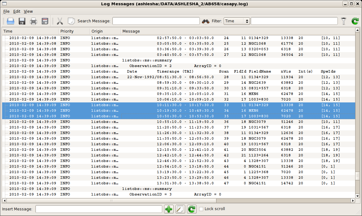
Using listobs and plotants we learn the source names, spectral windows, and viable reference antennas. A screenshot of the listobs output is given at right.
| Source | MKN6 |
| Amp Cal | 0134+329 = 3C48 |
| Phase Cal | 1003+830 |
| Central Antennas | VA27, VA09, VA23 |
| Spectral Window IDs | 10, 11 |
The selection of the spectral windows is key to getting the calibration right. Each science target in the multisource measurement set has a tuning respective of the source redshift, and the calibration observations are matched to those spectral windows. Were the spectral windows parameter (usually spw) left to its default value (all available spectral windows), many calibration routines would necessarily fail.
Editing the Data
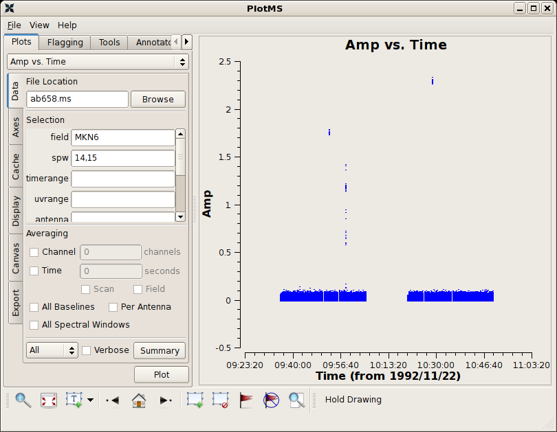
First inspect the data using plotms.
plotms(vis='ab658.ms', field='MKN6', xaxis='time', yaxis='amp')
There is some obvious junk isolated in time; see the screenshot at right. Follow the tutorial to flag discrepant data for the source and calibrators.
Calibration
Calibration of HI absorption spectra follows the basic techniques outlined in the continuum tutorial and HI emission tutorial.
First, set the flux of the amplitude calibrator. Notice that we are being careful to keep track of the spectral windows and not using the default spw.
# set the flux standard
setjy(vis='ab658.ms', field='0134+329', spw='10,11', modimage='')
Bandpass calibration comes next.
# bandpass calibration
bandpass(vis='ab658.ms', spw='10,11', caltable='ab658.bcal', gaintable='', gainfield='', interp='', field='0134+329', selectdata=False, bandtype='B', solint='inf', combine='scan', refant='VA27')
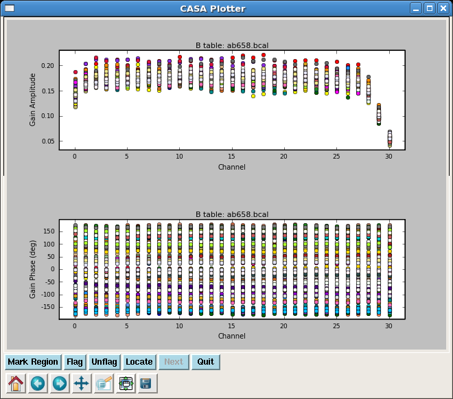
In order to perform the amplitude and phase calibrations, we'll need to inspect the bandpass response curve to select appropriate channels to average. We want to choose those channels where the response is relatively flat. The result of plotcal is shown at right: the bandpass is flat over channels 2:27.
# In CASA
%cpaste

# Press Enter or Return, then copy/paste all of the following:
# plot the bandpass calibration, amp vs channel
plotcal(caltable='ab658.bcal', spw='10,11', field='0134+329', subplot=211, yaxis='amp', showgui=True)

# plot the bandpass calibration, gain phase vs channel
plotcal(caltable='ab658.bcal', spw='10,11', field='0134+329', subplot=212, yaxis='phase', showgui=True)
--
The following steps generate amplitude and phase solutions for the calibrators, and the fluxscale is bootstrapped from the amplitude calibrator onto the phase calibrator, effectively turning the phase calibrator into a local flux calibrator for the science target.
# generate amplitude and gain solutions for phase and amplitude calibrators
gaincal(vis='ab658.ms', caltable='ab658.gcal', gaintable='ab658.bcal', gainfield='', interp='nearest', field='0134+329, 1003+830',
        spw='10:2~27, 11:2~27', selectdata=False, gaintype='G', solint='inf', combine='', calmode='ap', minsnr=1.0, refant='VA27')
# Bootstrap flux scale
fluxscale(vis='ab658.ms', fluxtable='MKN6.fluxscale', caltable='ab658.gcal', reference='0134+329', transfer='1003+830')
The task fluxscale will give the bootstrapped flux density of the phase calibrator. If all goes well, something like the following should appear in the log window.
Beginning fluxscale--(MSSelection version)-------
 Found reference field(s): 0134+329
 Found transfer field(s):  1003+830
 Flux density for 1003+830 in SpW=10 (freq=1.39215e+09 Hz) is: 0.492631 +/- 0.00341773 (SNR = 144.14, N = 52)
 Flux density for 1003+830 in SpW=11 (freq=1.3943e+09 Hz) is: 0.489476 +/- 0.00286404 (SNR = 170.904, N = 52)
 Storing result in ab658.fluxscale
We should inspect the calibration solutions to make sure they are reasonable, but we'll be cavalier and tread forward. Apply the calibrations to the science target and split that target into its own measurement set.
# apply calibrations to science target
applycal(vis='ab658.ms', gaintable=['MKN6.fluxscale','ab658.bcal'], gainfield=['1003+830', '*'], interp=['linear','nearest'], field='MKN6', spw='10,11', spwmap=[], selectdata=False)
# split out the corrected data column (which is placed in the data column in the new MS) for our science target.
split(vis='ab658.ms', outputvis='ab658-MKN6.split.ms', field='MKN6', spw='10:2~27, 11:2~27', datacolumn='corrected')
- spw='10:2~27, 11:2~27 : Note that we have selected only the inner channels, 2 through 27 for spectral windows 10, 11.
Continuum Subtraction
Ideally, we would use plotms to identify the channels where HI absorption is present (see the HI emission tutorial.) The absorption line is however weak and isolated against one of a number of radio continuum sources in the data; as such, the absorption is not apparent in averaged visibilities. Instead, we'll have to produce a dirty cube using clean and inspect the spectrum in the image domain.
Search for the Absorption Line
uvcontsub currently identifies continuum ranges by channel rather than frequency or velocity. We'll make two cubes, one for each spectral window. Note that the act of using split re-indexes the spectral windows and channels. Therefore spw='2~27' have been reindexed and are now spw='0~25' for both channels 10 & 11 (now reindexed as channels 0 & 1).
# image cube for spectral window 0
clean(vis='ab658-MKN6.split.ms', imagename='temp0', spw='0:0~25', mode='channel', nchan=-1, start=0, width=1, interpolation='nearest', niter=2000,
      cell=['0.4arcsec', '0.4arcsec'], phasecenter='J2000 06h52m12.2 +74d25m37')
# make a new image cube with spectral window 1
clean(vis='ab658-MKN6.split.ms', imagename='temp1', spw='1:0~25', mode='channel', nchan=-1, start=0, width=1, interpolation='nearest', niter=2000,
      cell=['0.4arcsec', '0.4arcsec'], phasecenter='J2000 06h52m12.2 +74d25m37')
It's not ordinarily necessary to give the phase center, but this is a good opportunity to use the regridding capabilities of clean. The data were originally taken in B1950 coordinates, and the observations followed the good practice of offsetting the pointing center slightly away from the source coordinates. Here, we specify the J2000 coordinates (looked up on NED) and allow clean to handle the precession and centering that we require.
The output cubes will go to temp0.image and temp1.image.
Now we can inspect the cube in viewer.
viewer(infile='temp0.image', displaytype='raster')
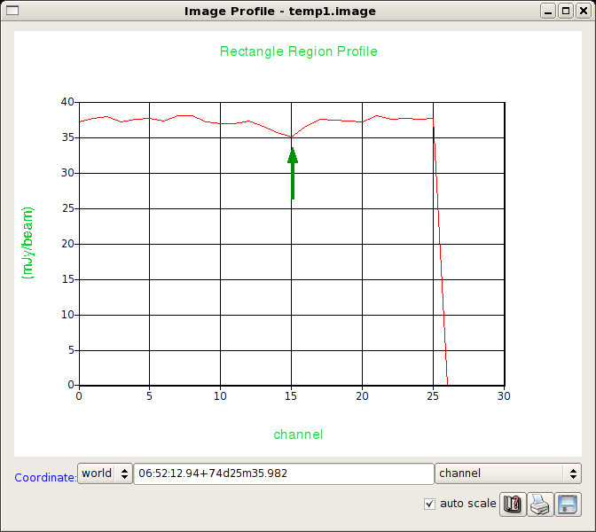
Now, use viewer to generate a spectrum. The source spectrum in spw = 1 is shown in the figure at right.
- If necessary. use the player buttons
 to scan through the channels until you see the source.
 - (Tools)Spectral Profile
- Right-click and drag a box around the source; the spectrum will appear in the Image Profile window.
- On the Image Profile window, change the velocity convention to Channel using the pull-down menu.
- Optional: Save the numerical data to a file. Click the save-as-text button
 and write the data to a file; for this example, we'll use temp0.txt.
Repeat for spw = 1.
viewer(infile='temp1.image', displaytype='raster')
Perform the Continuum Subtraction
Looking over the plots and text files, only channels 0~25 in either spectral window contain usable data. The absorption line is located in 1:15 and surrounding channels. Just to play it safe, we'll use the channels outside of 1:10~20 (spectral window 1, channels 10-20) to define the continuum for subtraction.
uvcontsub(vis='ab658-MKN6.split.ms', fitspw='0:0~25, 1:0~9; 21~25', solint='int', fitorder=1)
uvcontsub produces the uv subtracted measurement set:
- ab658-MKN6.split.ms.contsub (continuum-subtracted visibilities).
Imaging the Continuum Subtracted Cube
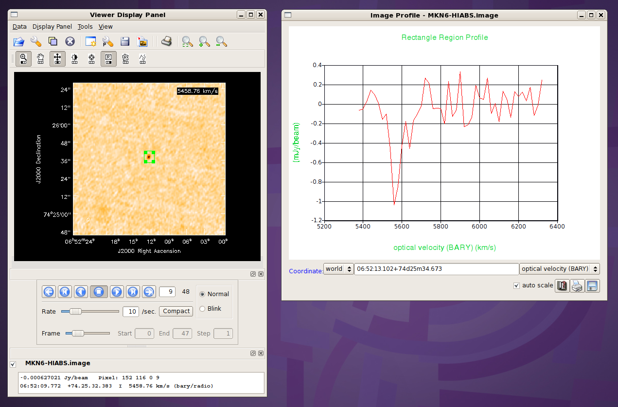
Inspecting the preliminary (continuum-containing) cubes, temp0.image and temp1.image, that we generated above, we can determine good parameters for the velocity axis. Here are the velocity options I came up with.
clean(vis='ab658-MKN6.split.ms.contsub', spw='', imagename='MKN6-HIABS', mode='velocity', nchan=-1, start='-252.349km/s', interpolation='linear', width='',
      outframe='bary', veltype='optical', restfreq='1420.405752MHz', niter=2000, threshold='1.0mJy', weighting='natural', cell=['0.4arcsec', '0.4arcsec'],
      phasecenter = 'J2000 06h52m12.2 +74d25m37')
- width= : Set the channel width equal to the first channel in the first spectral window.
- threshold='1.0mJy' : avoid over-cleaning since it appears that the channel rms is about 0.5 mJy/beam
- cell = ['0.4arcsec', '0.4arcsec'] : VLA-A configuration expects 1.5--2 arcsec beams. 0.4arcsec pixels ensure sampling the beam by better than 3x
The (viewer) results are illustrated in the figure at upper right.
Imaging the Continuum Dataset
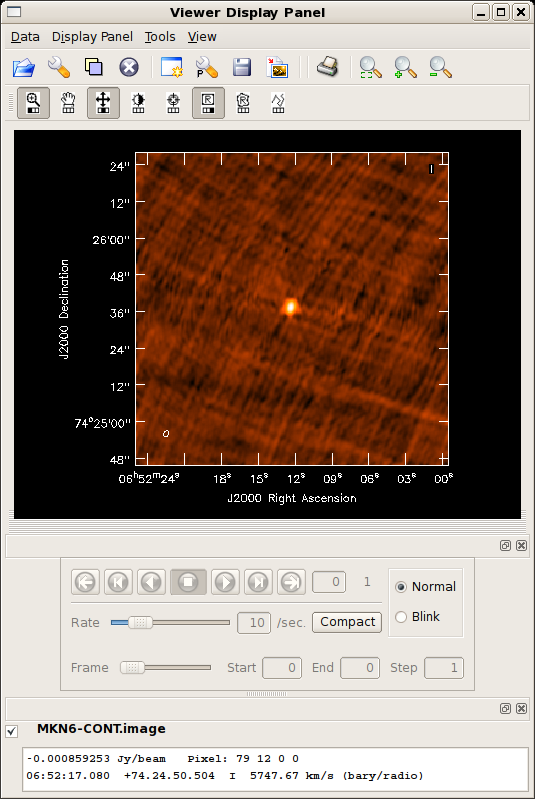
We can similarly image the continuum data with just a few changes of the clean parameters. Here, we call clean by selecting the spectral windows and channels pertaining to only the continuum.
clean(vis='ab658-MKN6.split.ms', mode='mfs', spw='0:0~25,1:0~9;21~25', imagename='MKN6-CONT', restfreq='1420.405752MHz', niter=2000,
      threshold='1.0mJy', weighting='natural', cell=['0.4arcsec', '0.4arcsec'], phasecenter = 'J2000 06h52m12.2 +74d25m37')
The result is shown at right. The continuum image needs some more help. Phase errors produce the 6-pointed star pattern surrounding the source and can be healed using self-calibration. The striping across the field is actually the combination of sidelobes from neighboring sources; these sidelobes can be suppressed by cleaning flanking fields.
Extract the Absorption Spectrum
viewer provides a handy first-look at the spectrum, but the extracted spectrum is an average over a spatial box. What we really want is the integrated spectrum, not the average. To do this, we'll use CASA's imstat, imval, and imhead tools to extract cube information to python variables and then let python build up the spectrum.
Extract the Spectrum: load the cube data into python arrays
First, we need to determine where in the cube to extract the spectrum; equivalently, we need to find the location of the minimum value in the cube. imstat is the tool for this.
cubeStat=imstat("MKN6-HIABS.image")
The variable cubeStat is now a python dictionary. To see what it contains, just enter the variable name:
cubeStat
and the following summary of cubeStat appears.
{'blc': array([0, 0, 0, 0], dtype=int32),
 'blcf': '06:52:24.903, +74.24.45.777, I, 1.39522e+09Hz',
 'flux': array([-0.05243921]),
 'max': array([ 0.00279196]),
 'maxpos': array([173,  82,   0,  33], dtype=int32),
 'maxposf': '06:52:07.732, +74.25.18.597, I, 1.39199e+09Hz',
 'mean': array([ -3.96712512e-07]),
 'medabsdevmed': array([ 0.00029433]),
 'median': array([ 0.]),
 'min': array([-0.01497807]),
 'minpos': array([127, 131,   0,   7], dtype=int32),
 'minposf': '06:52:12.299, +74.25.38.200, I, 1.39453e+09Hz',
 'npts': array([ 3145728.]),
 'quartile': array([ 0.00058867]),
 'rms': array([ 0.00047121]),
 'sigma': array([ 0.00047121]),
 'sum': array([-1.24794966]),
 'sumsq': array([ 0.69847239]),
 'trc': array([255, 255,   0,  47], dtype=int32),
 'trcf': '06:51:59.574, +74.26.27.778, I, 1.39063e+09Hz'}
These entries can be accessed individually like an array variable. For example, the following commands copy the x and y positions of the absorption line to scalar variables.
%cpaste

# Press Enter or Return, then copy/paste the following:
x2extract = cubeStat['minpos'][0]
y2extract = cubeStat['minpos'][1]
--
Now, extract the spectrum using imval.
%cpaste

# Press Enter or Return, then copy/paste the following:
extractBox = "%d,%d" % (x2extract, y2extract) # copy the position to a string
cubeSpec = imval("MKN6-HIABS.image", box=extractBox, stokes='I')
--
cubeSpec is another python dictionary, and the spectrum is stored in cubeSpec['data'].
Comment: The absorption line source is unresolved by this observation, or, to put it another way, is entirely contained within a synthesized beam. The extraction at a single spatial pixel gives the integrated spectrum and therefore changes units from surface brightness (mJy/beam) to flux density (mJy). However, the data have been forced into a rectangular grid, and there's no guarantee that the absorption minimum centers within a pixel. Better to use imfit to determine more accurately the position of the minimum, and perhaps re-clean with a new phasecenter. To avoid complicating the present tutorial, we'll just stick with the minimum in the current clean grid.
Generate the frequency axis
We can derive the frequency axis from the header.
# In CASA
%cpaste

# Press Enter or Return, then copy/paste the following:
import numpy # make sure vector and array arithmetic options are loaded
cubeHead = imhead("MKN6-HIABS.image", mode="list")
nSpec = cubeStat['trc'][3] + 1 # get the number of frequency channels.
f0 = float(cubeHead['crval4']) # reference freq in Hz
df = float(cubeHead['cdelt4']) # channel width in Hz
i0 = cubeHead['crpix4'] # reference pixel
freqSpec = (numpy.arange(nSpec) - i0)*df + f0
--
Plot the spectrum using matplotlib
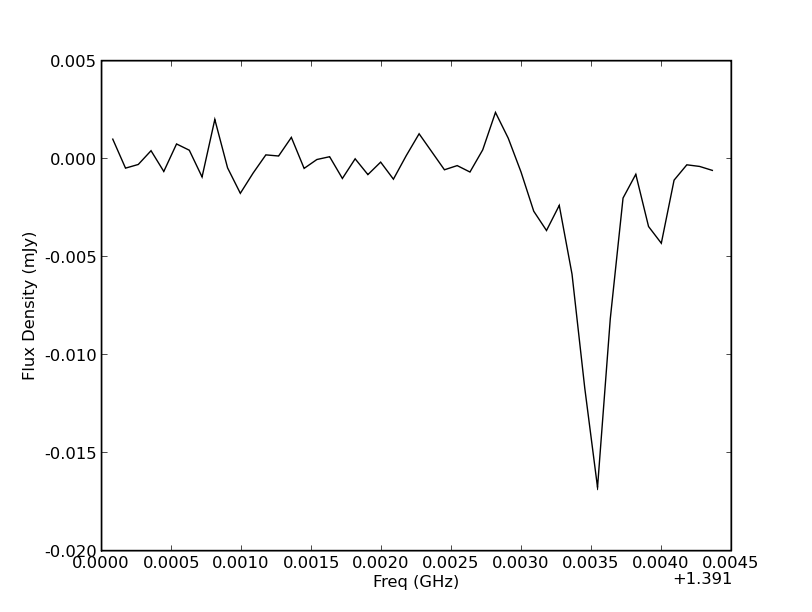
Now we have the spectrum stored in freqSpec, cubeSpec['data']. Use matplotlib.pyplot to plot the spectrum (see figure at right).
# In CASA
%cpaste

import matplotlib.pyplot as plt
plt.clf() # clear the plot (figure)
plt.plot(freqSpec/1.e9, cubeSpec['data'], 'k-')
plt.xlabel("Freq (GHz)")
plt.ylabel("Flux Density (mJy)")
plt.show()
--
A publication-quality figure: plot the spectrum against velocity
Nice, now let's make a velocity axis instead. We'll use the optical convention to convert frequency to velocity; the radio convention is offered as an alternative but is commented out.
# In CASA
%cpaste

import matplotlib.pyplot as plt
fRest = cubeHead['restfreq'][0]
velocity = 299792.458 * (fRest/freqSpec - 1.0) # optical convention, km/s
# velocity = 299792.458 * (1.0 - freqSpec/fRest) # radio convention, km/s
--
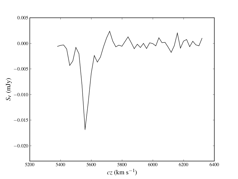
Plot the spectrum again, but this time try for publication-ready quality (see figure at right). This example is somewhat more clever to highlight the use of TeX typography in matplotlib. Note that you will have to have a compatible version of LaTeX installed for this to be successful.
# set up fonts
%cpaste

from matplotlib import rc
rc('font',**{'family':'serif','serif':['Times']})
rc('text', usetex=True)
plt.clf() # clear the plot (figure)
plt.plot(velocity, cubeSpec['data'], 'k-')
# the r prefix to the following format strings prevents \ from triggering an escape sequence,
#     like \n for line feed
plt.xlabel(r"$cz$ (km s$^{-1}$)",fontsize=16)
plt.ylabel(r"$S_{\nu}$ (mJy)",fontsize=16)
plt.ylim(-0.023,0.005)
plt.savefig("mkn6-abs.eps") # save the figure as encapsulated postscript, suitable for journals
plt.savefig("mkn6-abs.png") # save the figure as a bitmap, better suited for astro-ph
--
Save the spectrum to a text file
It's handy to have a simple, columnar text file to inspect and analyze later. Or perhaps you might want to analyze the spectrum outside of CASA. Numpy makes it easy to save and restore text files.
# First, combine the spectrum into a single array
%cpaste

spectrum = numpy.vstack((velocity, cubeSpec['data']))
numpy.savetxt("mrk6.txt", numpy.transpose(spectrum))
--
Here's a listing of the first few lines of mrk6.txt.
5.379999999489542461e+03 -5.940478877164423466e-04
5.399939886933506386e+03 -3.919676819350570440e-04
5.419882380281690530e+03 -3.093948180321604013e-04
5.439827480044931690e+03 -1.092202146537601948e-03
5.459775186734200361e+03 -4.310846794396638870e-03
5.479725500860732609e+03 -3.458642400801181793e-03
5.499678422935699928e+03 -7.933050510473549366e-04
5.519633953470603956e+03 -2.004600130021572113e-03
5.539592092976883578e+03 -8.163747377693653107e-03
5.559552841966238702e+03 -1.676503755152225494e-02
Here's how to restore that text file back into CASA (or python, for that matter).
%cpaste

# import numpy # if you haven't already
spectrum = numpy.loadtxt("mrk6.txt",dtype="float")
x = spectrum[:,0]
y = spectrum[:,1]
--
Last checked on CASA Version 5.1.1.