VLA Data Combination-CASA4.6.0: Difference between revisions
| Line 46: | Line 46: | ||
== Initial Imaging == | == Initial Imaging == | ||
To start with, we will | To start with, we will inspect the data and create separate images to better understand the image parameters such as integration time, resolution, and rms. | ||
Start CASA as usual via | Start CASA as usual via | ||
| Line 55: | Line 55: | ||
</source> | </source> | ||
As a first step, let's have a look at the {{listobs}} output for the different MeasurementSets. For example, the A-configuration MS had the following structure: | |||
<source lang="python"> | <source lang="python"> | ||
| Line 152: | Line 152: | ||
</pre> | </pre> | ||
We see that A-configuration contains only the central source, "J1745-2900" which is a different name for Sgr A*. The integration time | We see that A-configuration contains only the central source, "J1745-2900" which is just a different name for Sgr A*. The integration time amounts to only five minutes and the 16 spectral windows span a frequency range from 1.988 to 4.012GHz (when adding the bandwidth to the first channel of the last subband). Inspection of the other array configuration files show almost identical setups. Although the integration times between the different array configurations do not follow the 1:3:9 as we discussed in the previous section, we can still combine the data without any problems. In the end, having better signal to noise on the shorter baselines can only improve the overall, combined image. | ||
To better understand the data, let's check the uv-coverages of the three datasets. | |||
<source lang="python"> | <source lang="python"> | ||
| Line 167: | Line 167: | ||
plotuv(vis='VLA-SgrA-Sband-Cconfig.ms') | plotuv(vis='VLA-SgrA-Sband-Cconfig.ms') | ||
</source> | </source> | ||
The uv-coverages are shown in Fig. 1. The aspect ratio of each uv-coverage is not unity as Sgr A* is a very southern source. We also see that the longest baseline in each array differs by about a factor of 3 between the three configurations, as expected from the VLA A, B, and C configurations. | |||
{| | {| | ||
|[[Image:VLA-comb-A-uvcover_fld0.png|400px|thumb|left|'''Figure | |[[Image:VLA-comb-A-uvcover_fld0.png|400px|thumb|left|'''Figure 1a:''' <br />UV-coverage of A-configuration data.]] | ||
|[[Image:VLA-comb-B-uvcover_fld0.png|400px|thumb|left|'''Figure | |[[Image:VLA-comb-B-uvcover_fld0.png|400px|thumb|left|'''Figure 1b:''' <br />UV-coverage of B-configuration data.]] | ||
|[[Image:VLA-comb-C-uvcover_fld0.png|400px|thumb|left|'''Figure | |[[Image:VLA-comb-C-uvcover_fld0.png|400px|thumb|left|'''Figure 1c:''' <br />UV-coverage of C-configuration data.]] | ||
|} | |} | ||
To | |||
The next step is to determine the image quality, the synthesized beam, and the rms of each image. To do so, the images do not have to be perfect as we only would like to see how the combination will improve over the individual arrays. | |||
To keep things easy, we will use common cell sizes of 0.1 arcsec, images of 1280 pixels on each side, and we will {{clean}} 1000 iterations (see the [http://casaguides.nrao.edu/index.php/VLA_CASA_Imaging VLA CASA imaging guide for more sophisticated imaging parameter choices]): | |||
<source lang="python"> | <source lang="python"> | ||
Revision as of 22:47, 18 August 2016
This tutorial was created and tested using CASA 4.6.0
Introduction
A perfect image requires to measure all spatial scales which is equivalent to filling in the complete uv plane. Unfortunately, this can never be achieved with an aperture synthesis interferometer although a large number of baselines, long integration times, and multi-frequency-synthesis are all approaches to increase the uv-coverage. One method to obtain more baselines is to observe in different array configurations and to combine the data. Deconvolution algorithms are then given good starting conditions to interpolate over the gaps to achieve an improved image, an image that combines the surface brightness sensitivity of the compact baselines, with the spatial resolution of the extended baselines.
The VLA can be configured into four principal array configurations, A, B, C, and D. A is the most extended and D the most compact configuration. Consequently, A configuration data has the highest spatial resolution whereas D delivers the best surface brightness sensitivity and also images the largest scales of the sky distribution.
In this tutorial, we will combine data from three VLA configurations (A&B&C) that were obtained in a monitoring campaign of Sgr A*, the central, supermassive black hole of our Milky Way.
Typical Observing Times
When an object is being observed by the VLA in different configurations, integration times are ideally matched by their surface brightness sensitivity. Adjacent VLA configurations result in synthesized beams that differ in linear size by are approximately a factor of 3. The beam area is thus about 10 times different and the more extended configuration would ideally need to be 10 times longer than the most compact one. This, however, is frequently not very practical and it turns out that integration times that differ by factors of 3 are delivering data that can be combined satisfactorily as it matches the sensitivity of overlapping VLA visibilities when data are convolved to the same scales.
This rule, however, is only a guidance and any data that is being obtained from any configuration can be combined. Weighting will be primarily achieved by the image "Briggs" scheme that produces weights between the "natural" and "uniform" extremes, i.e., between weighting by the number of visibilities that are gridded in each cell and weighting by the cells themselves.
In addition, each visibility exhibits weights that should only depend on integration time, bandwidth, and system temperature. The VLA, however, currently does not measure Tsys and visibility weights between different observations will need to be adjusted as described below before they can be combined.
The Data
In the following we will combine three different datasets from the NRAO Monitoring of the Galactic Center/G2 Cloud Encounter. We will combine S-band A, B, and C configuration data. The data were all calibrated and the science target split out.
The calibrated measurement sets can be downloaded here:
https://casa.nrao.edu/Data/EVLA/SgrA/VLA-combination-SgrA-files.tar.gz (1.4GB)
As a first step, let's download the files, then untar:
# In Terminal
tar -xzvf VLA-combination-SgrA-files.tar.gz
This will unpack three MeasurementSets, one for each array configuration:
VLA-SgrA-Sband-Aconfig.ms

VLA-SgrA-Sband-Bconfig.ms

VLA-SgrA-Sband-Cconfig.ms
Initial Imaging
To start with, we will inspect the data and create separate images to better understand the image parameters such as integration time, resolution, and rms.
Start CASA as usual via
# In Terminal
casa
As a first step, let's have a look at the listobs output for the different MeasurementSets. For example, the A-configuration MS had the following structure:
# In CASA
listobs(vis='VLA-SgrA-Sband-Aconfig.ms')
##########################################
##### Begin Task: listobs            #####
listobs(vis="VLA-SgrA-Sband-Aconfig.ms",selectdata=True,spw="",field="",antenna="",
        uvrange="",timerange="",correlation="",scan="",intent="",
        feed="",array="",observation="",verbose=True,listfile="",
        listunfl=False,cachesize=50,overwrite=False)
================================================================================
           MeasurementSet Name:  /lustre/aoc/sciops/jott/casa/topicalguide/combination/test/VLA-SgrA-Sband-Aconfig.ms      MS Version 2
================================================================================
   Observer: lorant sjouwerman     Project: uid://evla/pdb/11434214
Observation: EVLA
Data records: 528000       Total elapsed time = 360 seconds
   Observed from   31-May-2014/09:07:57.0   to   31-May-2014/09:13:57.0 (UTC)
Compute subscan properties

   ObservationID = 0         ArrayID = 0
  Date        Timerange (UTC)          Scan  FldId FieldName             nRows     SpwIds   Average Interval(s)    ScanIntent
  31-May-2014/09:07:57.0 - 09:13:57.0    63      0 J1745-2900              528000  [0,3,4,5,6,7,8,9,10,11,12,13,14,15]  [3, 3, 3, 3, 3, 3, 3, 3, 3, 3, 3, 3, 3, 3] [OBSERVE_TARGET#UNSPECIFIED]
           (nRows = Total number of rows per scan)
Fields: 1
  ID   Code Name                RA               Decl           Epoch   SrcId      nRows
  0    NONE J1745-2900          17:45:40.038300 -29.00.28.06899 J2000   0         528000
Spectral Windows:  (14 unique spectral windows and 1 unique polarization setups)
  SpwID  Name           #Chans   Frame   Ch0(MHz)  ChanWid(kHz)  TotBW(kHz) CtrFreq(MHz) BBC Num  Corrs
  0      EVLA_S#A0C0#80     64   TOPO    1988.000      2000.000    128000.0   2051.0000       12  RR  LL
  3      EVLA_S#A0C0#83     64   TOPO    2372.000      2000.000    128000.0   2435.0000       12  RR  LL
  4      EVLA_S#A0C0#84     64   TOPO    2500.000      2000.000    128000.0   2563.0000       12  RR  LL
  5      EVLA_S#A0C0#85     64   TOPO    2628.000      2000.000    128000.0   2691.0000       12  RR  LL
  6      EVLA_S#A0C0#86     64   TOPO    2756.000      2000.000    128000.0   2819.0000       12  RR  LL
  7      EVLA_S#A0C0#87     64   TOPO    2884.000      2000.000    128000.0   2947.0000       12  RR  LL
  8      EVLA_S#B0D0#88     64   TOPO    2988.000      2000.000    128000.0   3051.0000       15  RR  LL
  9      EVLA_S#B0D0#89     64   TOPO    3116.000      2000.000    128000.0   3179.0000       15  RR  LL
  10     EVLA_S#B0D0#90     64   TOPO    3244.000      2000.000    128000.0   3307.0000       15  RR  LL
  11     EVLA_S#B0D0#91     64   TOPO    3372.000      2000.000    128000.0   3435.0000       15  RR  LL
  12     EVLA_S#B0D0#92     64   TOPO    3500.000      2000.000    128000.0   3563.0000       15  RR  LL
  13     EVLA_S#B0D0#93     64   TOPO    3628.000      2000.000    128000.0   3691.0000       15  RR  LL
  14     EVLA_S#B0D0#94     64   TOPO    3756.000      2000.000    128000.0   3819.0000       15  RR  LL
  15     EVLA_S#B0D0#95     64   TOPO    3884.000      2000.000    128000.0   3947.0000       15  RR  LL
Sources: 16
  ID   Name                SpwId RestFreq(MHz)  SysVel(km/s)
  0    J1745-2900          0     -              -
  0    J1745-2900          1     -              -
  0    J1745-2900          2     -              -
  0    J1745-2900          3     -              -
  0    J1745-2900          4     -              -
  0    J1745-2900          5     -              -
  0    J1745-2900          6     -              -
  0    J1745-2900          7     -              -
  0    J1745-2900          8     -              -
  0    J1745-2900          9     -              -
  0    J1745-2900          10    -              -
  0    J1745-2900          11    -              -
  0    J1745-2900          12    -              -
  0    J1745-2900          13    -              -
  0    J1745-2900          14    -              -
  0    J1745-2900          15    -              -
Antennas: 26:
  ID   Name  Station   Diam.    Long.         Lat.                Offset from array center (m)                ITRF Geocentric coordinates (m)
                                                                     East         North     Elevation               x               y               z
  0    ea01  N32       25.0 m   -107.37.22.0  +33.56.33.6       -441.7442     4689.9683      -16.9356 -1600781.062100 -5039347.430600  3558761.526300
  1    ea02  N64       25.0 m   -107.37.58.7  +34.02.20.5      -1382.3632    15410.1417      -40.6233 -1599855.668100 -5033332.388100  3567636.626500
  2    ea03  E64       25.0 m   -107.27.00.1  +33.50.06.7      15507.5911    -7263.7210       67.2006 -1587600.203200 -5050575.869700  3548885.404900
  3    ea04  E24       25.0 m   -107.35.13.4  +33.53.18.1       2858.1804    -1349.1324       13.7306 -1598663.094300 -5043581.396100  3553767.023200
  4    ea05  W08       25.0 m   -107.37.21.6  +33.53.53.0       -432.1181     -272.1470       -1.5057 -1601614.092200 -5042001.651900  3554652.509800
  5    ea06  N56       25.0 m   -107.37.47.9  +34.00.38.4      -1105.2076    12254.3155      -34.2423 -1600128.382500 -5035104.142000  3565024.679400
  6    ea07  N48       25.0 m   -107.37.38.1  +33.59.06.2       -855.2644     9405.9610      -25.9303 -1600374.875000 -5036704.207500  3562667.885900
  7    ea08  N16       25.0 m   -107.37.10.9  +33.54.48.0       -155.8517     1426.6442       -9.3792 -1601061.957400 -5041175.883000  3556058.040000
  8    ea09  W64       25.0 m   -107.46.20.1  +33.48.50.9     -14240.7638    -9606.2696       17.1066 -1616361.587500 -5042770.516600  3546911.446900
  9    ea10  E40       25.0 m   -107.32.35.4  +33.52.16.9       6908.8305    -3240.7192       39.0202 -1595124.923100 -5045829.467200  3552210.703600
  10   ea11  W24       25.0 m   -107.38.49.0  +33.53.04.0      -2673.3552    -1784.5888       10.4757 -1604008.749300 -5042135.808900  3553403.716000
  11   ea12  N09       25.0 m   -107.37.07.8  +33.54.19.0        -77.4204      530.6453       -5.5755 -1601139.471200 -5041679.039700  3555316.553900
  12   ea13  W56       25.0 m   -107.44.26.7  +33.49.54.6     -11333.2004    -7637.6771       15.3707 -1613255.393400 -5042613.099800  3548545.915000
  13   ea14  E08       25.0 m   -107.36.48.9  +33.53.55.1        407.8298     -206.0320       -3.2196 -1600801.931000 -5042219.386500  3554706.431200
  14   ea15  E56       25.0 m   -107.29.04.1  +33.50.54.9      12327.6313    -5774.7469       42.6153 -1590380.611000 -5048810.243300  3550108.432300
  15   ea17  E32       25.0 m   -107.34.01.5  +33.52.50.3       4701.6413    -2209.7152       25.2066 -1597053.135800 -5044604.681200  3553058.995000
  16   ea18  E72       25.0 m   -107.24.42.3  +33.49.18.0      19041.8717    -8769.2047        4.7262 -1584460.871200 -5052385.599800  3547600.000100
  17   ea19  W16       25.0 m   -107.37.57.4  +33.53.33.0      -1348.7109     -890.6216        1.3005 -1602592.853600 -5042054.996800  3554140.704800
  18   ea20  N40       25.0 m   -107.37.29.5  +33.57.44.4       -633.6074     6878.6018      -20.7693 -1600592.756000 -5038121.357300  3560574.853200
  19   ea21  E48       25.0 m   -107.30.56.1  +33.51.38.4       9456.6097    -4431.6564       37.9341 -1592894.077600 -5047229.138200  3551221.206000
  20   ea22  N24       25.0 m   -107.37.16.1  +33.55.37.7       -290.3752     2961.8594      -12.2389 -1600930.087800 -5040316.396400  3557330.387200
  21   ea23  W72       25.0 m   -107.48.24.0  +33.47.41.2     -17419.4740   -11760.2758       14.9538 -1619757.312900 -5042937.664400  3545120.392300
  22   ea24  W48       25.0 m   -107.42.44.3  +33.50.52.1      -8707.9403    -5861.7877       15.5282 -1610451.925800 -5042471.125800  3550021.055800
  23   ea25  W32       25.0 m   -107.39.54.8  +33.52.27.2      -4359.4392    -2923.1244       11.7721 -1605808.634900 -5042230.089000  3552459.209500
  24   ea26  W40       25.0 m   -107.41.13.5  +33.51.43.1      -6377.9880    -4286.7769        8.2038 -1607962.463800 -5042338.190100  3551324.947500
  25   ea28  E16       25.0 m   -107.36.09.8  +33.53.40.0       1410.0378     -673.4764       -0.7821 -1599926.107500 -5042772.979700  3554319.790400
##### End Task: listobs              #####
##########################################
We see that A-configuration contains only the central source, "J1745-2900" which is just a different name for Sgr A*. The integration time amounts to only five minutes and the 16 spectral windows span a frequency range from 1.988 to 4.012GHz (when adding the bandwidth to the first channel of the last subband). Inspection of the other array configuration files show almost identical setups. Although the integration times between the different array configurations do not follow the 1:3:9 as we discussed in the previous section, we can still combine the data without any problems. In the end, having better signal to noise on the shorter baselines can only improve the overall, combined image.
To better understand the data, let's check the uv-coverages of the three datasets.
# In CASA
# A-config:
plotuv(vis='VLA-SgrA-Sband-Aconfig.ms')
#
# B-config
plotuv(vis='VLA-SgrA-Sband-Bconfig.ms')
#
# C-config:
plotuv(vis='VLA-SgrA-Sband-Cconfig.ms')
The uv-coverages are shown in Fig. 1. The aspect ratio of each uv-coverage is not unity as Sgr A* is a very southern source. We also see that the longest baseline in each array differs by about a factor of 3 between the three configurations, as expected from the VLA A, B, and C configurations.
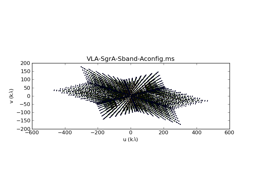 UV-coverage of A-configuration data. |
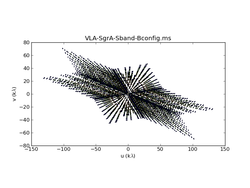 UV-coverage of B-configuration data. |
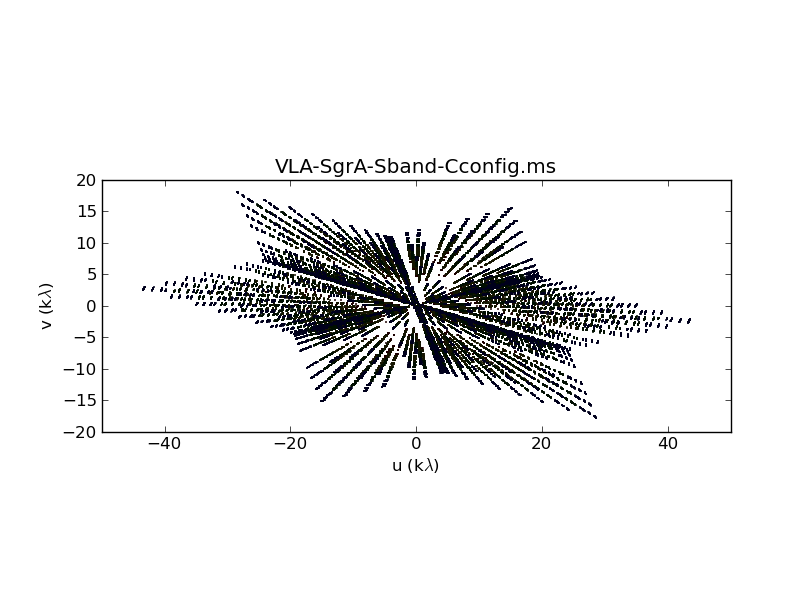 UV-coverage of C-configuration data. |
The next step is to determine the image quality, the synthesized beam, and the rms of each image. To do so, the images do not have to be perfect as we only would like to see how the combination will improve over the individual arrays.
To keep things easy, we will use common cell sizes of 0.1 arcsec, images of 1280 pixels on each side, and we will clean 1000 iterations (see the VLA CASA imaging guide for more sophisticated imaging parameter choices):
# In CASA
# A-config:
clean(vis='VLA-SgrA-Sband-Aconfig.ms', imagename='SgrA-Aonly',field='J1745-2900',
      mode='mfs',cell='0.1arcsec',imsize=[1280,1280],niter=1000,weighting='briggs',robust=0)
#
# B-config
clean(vis='VLA-SgrA-Sband-Bconfig.ms', imagename='SgrA-Bonly',field='J1745-2900',
      mode='mfs',cell='0.1arcsec',imsize=[1280,1280],niter=1000,weighting='briggs',robust=0)
#
# C-config:
clean(vis='VLA-SgrA-Sband-Cconfig.ms', imagename='SgrA-Conly',field='J1745-2900',
      mode='mfs',cell='0.1arcsec',imsize=[1280,1280],niter=1000,weighting='briggs',robust=0)
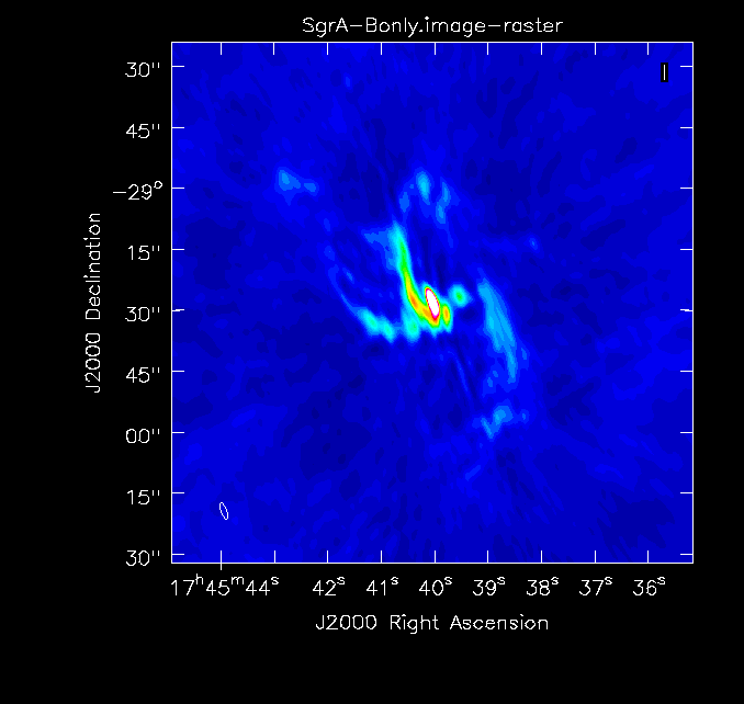
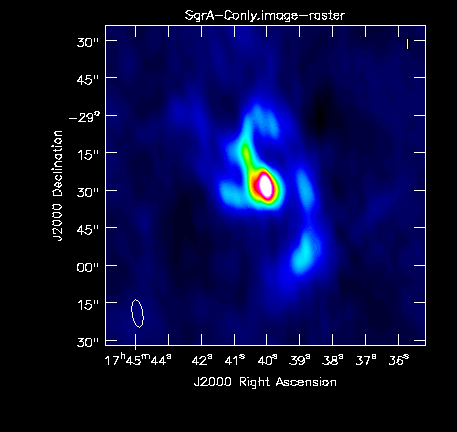
The clean images are not yet ideal. In particular, there are streaks across the entire image. After comparing their orientation with the psf, it is clear that they result from imperfect uv-coverage due to the short integration times of the observations. To get better images, we recommend the setting of clean boxes in the interactive=True interactive mode.
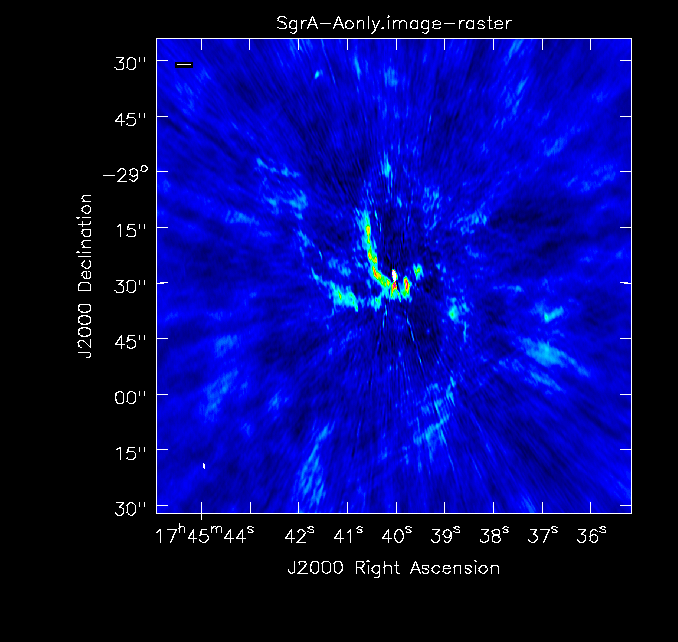 Simple image of A-configuration data. |
 Simple image of B-configuration data. |
 Simple image of C-configuration data. |
For the basic parameters, we find the following:
For A-configuration the synthesized beam is: 1.44" x 0.40" , the rms: ~0.8mJy, and the peak flux of Sgr A* is: 0.712 Jy
For B-configuration the synthesized beam is: 4.33" x 1.34" , the rms: ~0.7mJy, and the peak flux of Sgr A* is: 0.691 Jy
For C-configuration the synthesized beam is: 11.02" x 4.20" , the rms: ~0.6mJy, and the peak flux of Sgr A* is: 1.35 Jy
Although the cleaning could have been better, the image quality of all three datasets is good enough for combination. In fact, adding all uv-coverages together will increase the image quality substantially.
Check and Adjust the Visibility Weights
The VLA does not measure system temperatures and does not have calibrated weights. However, the relative sensitivity within an observation is measured by the gain, so weights of a continuous observation are consistent. It is important though to adjust the weights between different observations. The task statwt in CASA will recalculate the visibility weights based on their rms. This task needs to be executed on each visibility dataset. Typically the default setting works quite well for continuum observations. Note that for spectral line data one should specify the fitspw parameter to exclude the line from the calculations as it will be down-weighes otherwise.
Let's have a look at the weights before running statwt:
# In CASA
# A-config:
plotms(vis='VLA-SgrA-Sband-Aconfig.ms',spw='3',averagedata=T,
       avgchannel='64',xaxis='uvwave',yaxis='wt',coloraxis='antenna1')
#
# B-config
plotms(vis='VLA-SgrA-Sband-Bconfig.ms',spw='3',averagedata=T,
       avgchannel='64',xaxis='uvwave',yaxis='wt',coloraxis='antenna1')
#
# C-config:
plotms(vis='VLA-SgrA-Sband-Cconfig.ms',spw='3',averagedata=T,
       avgchannel='64',xaxis='uvwave',yaxis='wt',coloraxis='antenna1')
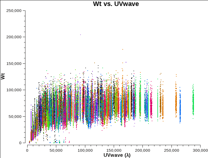 A-config Original Weights. |
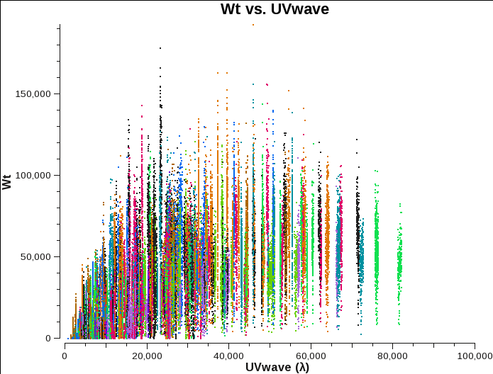 B-config Original Weights. |
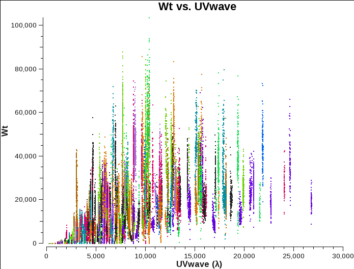 C-config Original Weights. |
We will use the default setting of statwt (calculation for each spw and scan per baseline). As statwt will overwrite the WEIGHT column, we first will create copies of our data:
# In Linux
cp -r VLA-SgrA-Sband-Aconfig.ms VLA-SgrA-Sband-Aconfig-statwt.ms
cp -r VLA-SgrA-Sband-Bconfig.ms VLA-SgrA-Sband-Bconfig-statwt.ms
cp -r VLA-SgrA-Sband-Cconfig.ms VLA-SgrA-Sband-Cconfig-statwt.ms
# In CASA
# A-config:
statwt(vis='VLA-SgrA-Sband-Aconfig-statwt.ms')
#
# B-config
statwt(vis='VLA-SgrA-Sband-Bconfig-statwt.ms')
#
# C-config:
statwt(vis='VLA-SgrA-Sband-Cconfig-statwt.ms')
CASA will come up with a message that the CORRECTED column is not found and that DATA is being used. This is fine as indeed there's only a DATA column present in the MS, which is thus the one to calculate the new weights from.
# In CASA
# A-config:
plotms(vis='VLA-SgrA-Sband-Aconfig-statwt.ms',spw='3',averagedata=T,
       avgchannel='64',xaxis='uvwave',yaxis='wt',coloraxis='antenna1')
#
# B-config
plotms(vis='VLA-SgrA-Sband-Bconfig-statwt.ms',spw='3',averagedata=T,
       avgchannel='64',xaxis='uvwave',yaxis='wt',coloraxis='antenna1')
#
# C-config:
plotms(vis='VLA-SgrA-Sband-Cconfig-statwt.ms',spw='3',averagedata=T,
       avgchannel='64',xaxis='uvwave',yaxis='wt',coloraxis='antenna1')
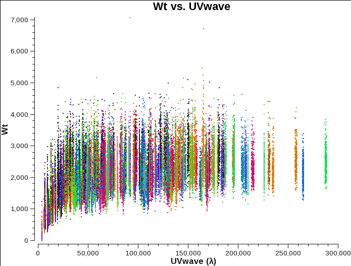 A-config Original Weights. |
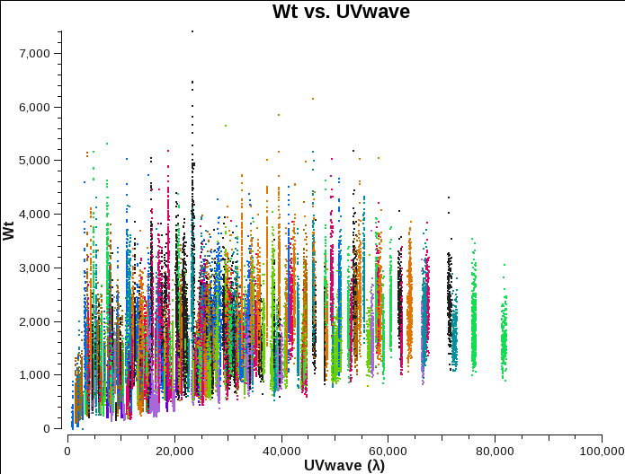 B-config Original Weights. |
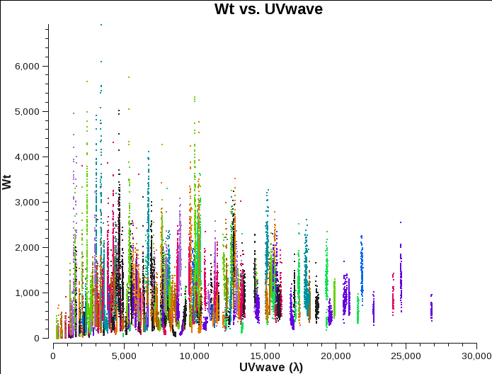 C-config Original Weights. |
Removal of the variable Sgr A* point source
This step is only necessary for our case which includes a variable source. In most cases, one can skip this step.
As we have seen in the initial imaging step, Sgr A* is a variable sourcce. Unfortunately, this also introduces some problems with the visibilities as the different uv points will then also show different values. Cleaning will be difficult in such a situation. We therefore will remove Sgr A* in each dataset and intrduce an averaged value later.
This will be done by creating a component list, that includes only a point source at the position of Sgr A*. The component list will then be inserted into the respective MS into the model column via ft, and uvsub will subtract the point source model from the CORRECTED data column. Since there's no CORRECTED column to start with, uvsub will create it. Note that that imples that running uvsub twice will oversubtract. So we recommend to again, make copies of the previous datasets.
# In Linux
cp -r VLA-SgrA-Sband-Aconfig-statwt.ms VLA-SgrA-Sband-Aconfig-statwt-sub.ms
cp -r VLA-SgrA-Sband-Bconfig-statwt.ms VLA-SgrA-Sband-Bconfig-statwt-sub.ms
cp -r VLA-SgrA-Sband-Cconfig-statwt.ms VLA-SgrA-Sband-Cconfig-statwt-sub.ms
Let's start with the A-configuration data and create a component list:
# In CASA
cl.addcomponent(flux=0.712, fluxunit='Jy',shape='point', dir='J2000 17:45:40.03599 -29.00.28.1699')
cl.rename('component-SgrA-A.cl')
cl.close()
Now we have a file 'component-SgrA-A.cl' that we attach to the model column of the file:
# In CASA
ft(vis='VLA-SgrA-Sband-Aconfig-statwt-sub.ms', complist='component-SgrA-A.cl')
And finally we will subtract the model from the data:
# In CASA
uvsub(vis='VLA-SgrA-Sband-Aconfig-statwt-sub.ms')
Note that to revert back to the original state, one could split out the DATA column and strip the MODEL and the point source subtracted CORRECTED column.
Let's repeat the steps for B-configuration:
# In CASA
cl.addcomponent(flux=0.691, fluxunit='Jy',shape='point', dir='J2000 17:45:40.03599 -29.00.28.1699')
cl.rename('component-SgrA-B.cl')
cl.close()
#
ft(vis='VLA-SgrA-Sband-Bconfig-statwt-sub.ms', complist='component-SgrA-B.cl')
#
uvsub(vis='VLA-SgrA-Sband-Bconfig-statwt-sub.ms')
And for C-configuration:
# In CASA
cl.addcomponent(flux=1.35, fluxunit='Jy',shape='point', dir='J2000 17:45:40.03599 -29.00.28.1699')
cl.rename('component-SgrA-C.cl')
cl.close()
#
ft(vis='VLA-SgrA-Sband-Cconfig-statwt-sub.ms', complist='component-SgrA-C.cl')
#
uvsub(vis='VLA-SgrA-Sband-Cconfig-statwt-sub.ms')
Finally, we will add back in a point source with a canonical 1Jy to bring back Sgr A*. reverse=T will add instead of subtract the model in uvsub.
# In CASA
cl.addcomponent(flux=1, fluxunit='Jy',shape='point', dir='J2000 17:45:40.03599 -29.00.28.1699')
cl.rename('component-SgrA.cl')
cl.close()
#
# A-config
#
ft(vis='VLA-SgrA-Sband-Aconfig-statwt-sub.ms', complist='component-SgrA.cl')
#
uvsub(vis='VLA-SgrA-Sband-Aconfig-statwt-sub.ms',reverse=T)
#
# B-config
#
ft(vis='VLA-SgrA-Sband-Bconfig-statwt-sub.ms', complist='component-SgrA.cl')
#
uvsub(vis='VLA-SgrA-Sband-Bconfig-statwt-sub.ms',reverse=T)
#
# C-config
#
ft(vis='VLA-SgrA-Sband-Cconfig-statwt-sub.ms', complist='component-SgrA.cl')
#
uvsub(vis='VLA-SgrA-Sband-Cconfig-statwt-sub.ms',reverse=T)
Image Combined Data
We can now make a combined image of all thre re-weighted datasets. The data could be combined with concat, but this is in fact not needed. clean will take care of the combination. By default, clean will image the data in the CORRECTED column, i.e. it will use the data where we subtracted the point source earlier.
To start with, we will just fill in the uv-plane, all relative weighting between the different array configurations will be performed with the robust weights. Note that the flux value for Sgr A* will also be a weighted mean of the three different datasets.
First, let's check the new uv-coverage. TO do so, we need to concatenate the data:
# In CASA
concat(vis=['VLA-SgrA-Sband-Aconfig-statwt-sub.ms','VLA-SgrA-Sband-Bconfig-statwt-sub.ms','VLA-SgrA-Sband-Cconfig-statwt-sub.ms'],concatvis='VLA-SgrA-Sband-combined.ms')
# In CASA
plotuv(vis='VLA-SgrA-Sband-combined.ms')
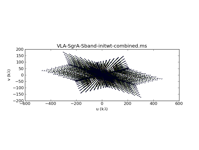 Combined uv-coverage. |
clean also accepts multiple files. We could use the concatenated visibilities that we just created, but let's simply use all three measurement sets for input.
# In CASA
clean(vis=['VLA-SgrA-Sband-Aconfig-statwt-sub.ms','VLA-SgrA-Sband-Bconfig-statwt-sub.ms','VLA-SgrA-Sband-Cconfig-statwt-sub.ms'],
      imagename='SgrA-all',field='J1745-2900',mode='mfs',cell='0.1arcsec',imsize=[1280,1280],niter=5000,
      threshold='5mJy',weighting='briggs',robust=0)
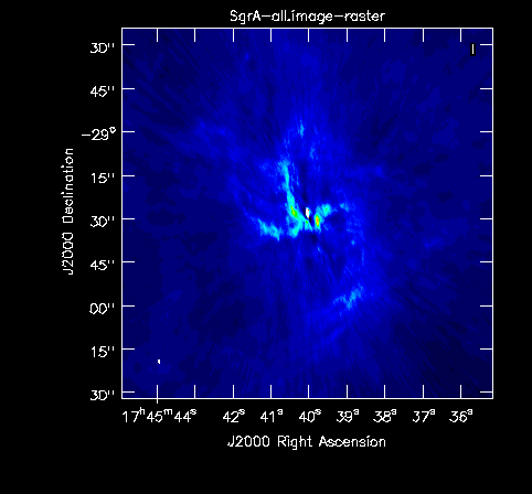 Combined image. |
The resulting image has a beam size of 1.58" x 0.50", very similar to the resolution of A-confguration only. This is what we want to achieve. The rms is better than A-only and there are clearly many more scales in the image. This is pretty good combination product.
The image can still be improved. For simplicity, we did not use any interactive cleaning above, but we highly recommend it for the final images. Improvements can also be obtained, e.g. by adjusting the image weights (robust parameter), adding a taper, or weighting the different datasets against each other (using concat). Wide-band imaging and multi-scale imaging will also improve the results. We refer to the VLA CASA Imaging Guide for more details.
Last checked on CASA Version 4.6.0