VLA CASA Imaging-CASA4.5.2

Imaging

This tutorial is about imaging techniques in CASA.

We will be utilizing data taken with the Karl G. Jansky, Very Large Array, of a supernova remnant G055.7+3.4.. The data were taken on August 23, 2010, in the first D-configuration for which the new wide-band capabilities of the WIDAR (Wideband Interferometric Digital ARchitecture) correlator were available. The 8-hour-long observation includes all available 1 GHz of bandwidth in L-band, from 1-2 GHz in frequency.

We will skip the calibration process in this guide, as examples of calibration can be found in several other guides, including the EVLA Continuum Tutorial 3C391 guide.

A copy of the calibrated data (1.2GB) can be downloaded from http://casa.nrao.edu/Data/EVLA/SNRG55/SNR_G55_10s.calib.tar.gz 

Your first step will be to unzip and untar the file in a terminal (before you start CASA):

tar -xzvf  SNR_G55_10s.calib.tar.gz

Then start casa as usual via the casa command which will bring up the ipythin interface and launches the logger.

The CLEAN Algorithm

The CLEAN major and minor cycles, indicating the steps undertaken during gridding, projection algorithms, and creation of images.

The CLEAN algorithm, developed by J. Högbom (1974) enabled the synthesis of complex objects, even if they have relatively poor Fourier uv-plane coverage. Poor coverage occurs with partial earth rotation synthesis, or with arrays composed of few antennas. The "dirty" image is formed by a simple Fourier inversions of the sampled visibility data, with each point on the sky being represented by a suitably scaled and centered PSF (Point Spread Function, sometimes called the dirty beam). This algorithm attempts to interpolate from the measured (u,v) points across gaps in the (u,v) coverage. It, in short, provides solutions to the convolution equation by representing radio sources by a number of point sources in an empty field.

The brightest points are found by performing a cross-correlation between the dirty image, and the PSF. The brightest parts are subtracted, and the process is repeated again for the next brighter sources. A large part of the work in CLEAN involves shifting and scaling the dirty beam.

The clean algorithm works well with points sources, as well as most extended objects. Where it can fall short is in speed, as convergence can be slow for extended objects, or for images containing several bright point sources. A solution to deconvolve these images would be, e.g. multiscale cleaning, which uses extended kernels for subtraction, not only the pure PSF.

For single pointings, CASA uses the Cotton-Schwab cleaning algorithm in the task clean (imagermode='csclean'), which breaks the process into major and minor cycles (see image). To start with, the visibilities are gridded, weighted, and Fourier transformed to create an (dirty) image. Then the minor cycle operates in the image domain to find the clean components that are added to the clean model. The image is then Fourier transformed back to the visibility domain, degridded and the clean model is being subtracted. This creates a new residual that is then gridded and FFT'ed again to the image domain for the next iteration. The gridding, FFT, degridding and subtraction processes form the major cycle.

This iterative process is being continued until a stopping criterium is being reached, such as a maximum number of clean components, or a flux threshold in the residual image.

In CASA clean, two versions of PSF can be used (parameter psfmode): hogbom uses the full sized PSF for subtraction. This is a thorough but slow method. psfmode='clark' uses a smaller beam patch which increases the speed. The patch size and length of the minor cycle are internally chosen such that the clean converges well without giving up the speed improvement. It is thus the default option in clean.

In a final step, clean derives a Gaussian fit to the inner part of the PSF, which defines the clean beam. The clean model is then convolved with the clean beam and added to the last residual image to create the final image.

Note that we are currently developing a refactored clean, called tclean. It has a better interface, and provides more possible combinations of algorithms. It also allows for process computing parallelization of the imaging and deconvolution. Eventually, tclean will replace the current clean task, but for now, we will stick with the original clean, as tclean is experimental and under testing at the moment.

For more details on imaging and deconvolution, you can refer to the Astronomical Society of the Pacific Conference Series book entitled Synthesis Imaging in Radio Astronomy II. The chapter on Deconvolution may prove helpful.

The CASA cookbook chapter on Synthesis Imaging provides a wealth of information, more specific for the CASA implementation of clean and related tasks.

Weights and Tapering

u,v coverage for the 8-hour observation of the supernova remnant G055.7+3.4

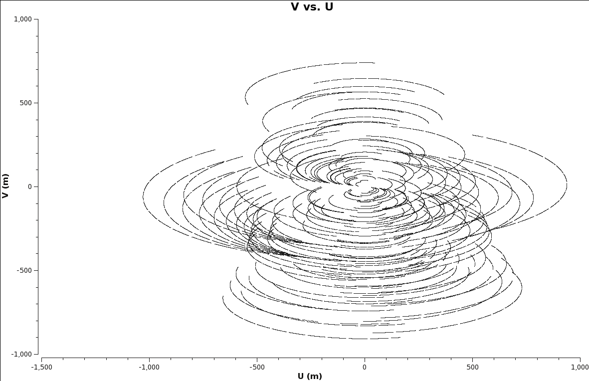
When imaging data, a map is created associating the visibilities with the image. The sampling function, which is a function of the visibilities, is modified by a weight function. [math]\displaystyle{ S(u,v) \to S(u,v)W(u,v) }[/math].

This process can be considered a convolution. The convolution map, is the weights by which each visibility is multiplied by before gridding is undertaken. Due to the fact that each VLA antenna performs slightly differently, different weights should be applied to each antenna. Therefore, the weight column in the data table reflects how much weight each corrected data sample should receive.

There are different options for [math]\displaystyle{ W(u,v) }[/math] (parameter weighting in clean):

1. Natural: The weight function can be described as [math]\displaystyle{ W(u,v) = 1/ \sigma^2 }[/math], where [math]\displaystyle{ \sigma^2 }[/math] is the noise variance. Natural weighting will maximize point source sensitivity, and provide the lowest rms noise within an image, as well as the highest signal-to-noise. It will also generally give more weight to short baselines, thus the synthesized beam will be large. This form of weighting is the default within the clean task.

2. Uniform: The weight function can be described as [math]\displaystyle{ W(u,v) = W(u,v) / W_k }[/math], where [math]\displaystyle{ W_k }[/math] represents the local density of (u,v) points, otherwise known as the gridded weights. This form of weighting will increase the influence of data with lower weight, filling the (u,v) plane more uniformly, thereby reducing sidelobe levels in the field-of-view, but increasing the rms image noise. More weight is given to long baselines, therefore increasing angular resolution. Point source sensitivity is degraded due to the downweighting of some data.

3. Briggs: A flexible weighting scheme, that is a variant of uniform, and avoids giving too much weight to (u,v) points with a low natural weight. Weight function can be described as [math]\displaystyle{ W(u,v) = 1/ \sqrt{1+S_N^2/S_{thresh}^2} }[/math], where [math]\displaystyle{ S_N }[/math] is the natural weight of the cell, [math]\displaystyle{ S_{thresh} }[/math] is a threshold. A high threshold will go to a natural weight, where as a low threshold will go to a uniform weight. This form of weighting also has adjustable parameters. The robust parameter will give variation between resolution and maximum point source sensitivity. It's value can range from -2.0 (close to uniform weight) to 2.0 (close to natural weight). By default, the parameter is set to 0.0, which gives a good trade-off.

Table summarizing the effects of using weights and tapering.

Tapering: In conjunction with weighting, we can include the uvtaper parameter within clean, which will control the radial weighting of visibilities, in the uv-plane. This in effect, reduces the visibilities, with weights decreasing as a function of uv-radius. The tapering will apodize, or filter/change the shape of the weight function (which is itself a Gaussian), which can be expressed as:
[math]\displaystyle{ W(u,v) = e^{-(u^2+v^2)/t^2} }[/math], where t is the adjustable tapering parameter. This process can smooth the image plane, give more weight to short baselines, but in turn degrade angular resolution. Due to the downweight of some data, point source sensitivity can be degraded. If your observation was sampled by short baselines, tapering may improve sensitivity to extended structures.

Primary and Synthesized Beam

The primary beam of a single antenna defines the sensitivity of the field of view. For the VLA antennas it can be approximated by a Gaussian with FWHM equal to [math]\displaystyle{ 90*\lambda_{cm} }[/math] or [math]\displaystyle{ 45/ \nu_{GHz} }[/math]. But note that there are sidelobes beyond the Gaussian kernel that are sensitive to bright sources (see below). Taking our observed frequency to be the middle of the band, 1.5GHz, our primary beam will be around 30 arcmin. Note that if your science goal is to image a source, or field of view that is significantly larger than the FWHM of the VLA primary beam, then creating a mosaic from a number of pointings would be best. For a tutorial on mosaicing, see the 3C391 tutorial.

Since our observation was taken in D-configuration, we can check the Observational Status Summary's section on VLA resolution to find that the synthesized beam will be around 46 arcsec. We want to oversample the synthesized beam by a factor of around five, so we will use a cell size of 8 arcsec.

Since this field contains bright point sources significantly outside the primary beam, we will create images that are 170 arcminutes on a side ([8arcsec * Cell Size]*[1arcmin / 60arsec]), or almost 6x the size of the primary beam. This is ideal for showcasing both the problems inherent in such wide-band, wide-field imaging, as well as some of the solutions currently available in CASA to deal with these issues.

First, it's worth considering why we are even interested in sources which are far outside the primary beam. This is mainly due to the fact that the EVLA, with its wide bandwidth capabilities, is quite sensitive even far from phase center -- for example, at our observing frequencies in L-band, the primary beam gain is as much as 10% around 1 degree away. That means that any imaging errors for these far-away sources will have a significant impact on the image rms at phase center. The error due to a source at distance R can be parametrized as:

[math]\displaystyle{ \Delta(S) = S(R) \times PB(R) \times PSF(R) }[/math]

A dirty image of the supernova remnant G55.7+3.4 in greyscale (left), and the point spread function (PSF), also known as the dirty beam (right).

So, for R = 1 degree, source flux S(R) = 1 Jy, [math]\displaystyle{ \Delta(S) }[/math] = 1 mJy − 100 [math]\displaystyle{ {\mu} }[/math]Jy. Clearly, this will be a source of significant error.

Strong sources in the primary beam sidelobes can also throw synthesized beam sidelobes in the central image. Cleaning far away from the phase center may thus become important in the vicinity of strong sources, in particular at the lower frequency bands where non-thermal emission dominates.

Clean Output Images

clean creates a number of output images. For an imagename='galaxy', this would be:

galaxy.image the residual + the model convolved with the clean beam. This is the main resulting image (unit: Jy/clean beam).
galaxy.residual the residual after subtracting the clean model (unit: Jy/dirty beam).
galaxy.model the clean model, not convolved (unti: Jy/pixel).
galaxy.psf the point-spread function aka dirty beam
galaxy.flux the normalized sensitivity map. For single pointings this corresponds to the primary beam.
galaxy.pbcoverage (only for mosaics). The primary beam response of the pointings combined.

Note: If an image file is present and given in imagename, clean will use that image as a starting point. If you want a fresh clean, first remove all images of that name using 'rmtables()':

# In CASA
rmtables('galaxy.*')

This method is preferable over 'rm -rf' as it also clears the cache.

Dirty Image

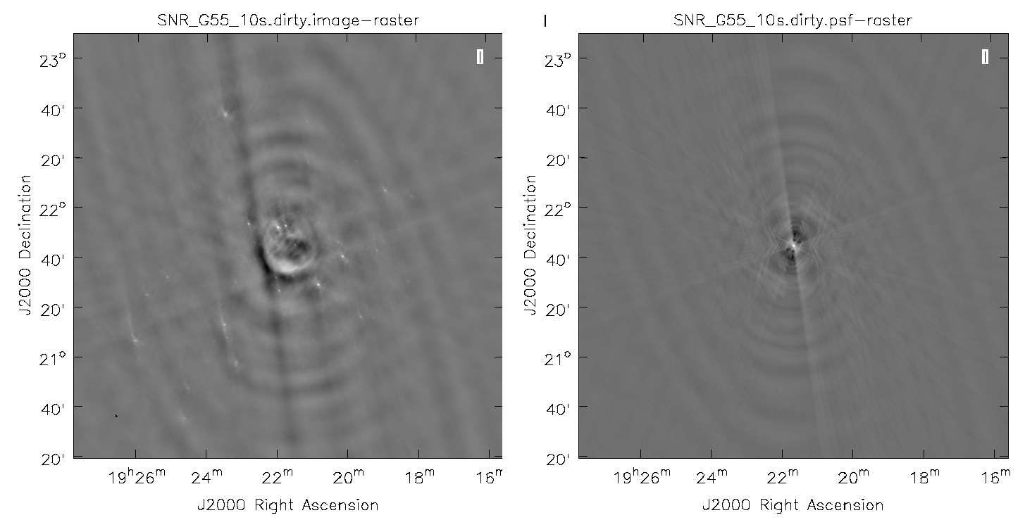
First, we will create a dirty image to see the improvements as we step through several cleaning algorithms and parameters. The dirty image is the true image, convolved with the dirty beam (PSF). We will do this by running CLEAN with niter=0, which controls the number of iterations done in the minor cycle.

# In CASA
clean(vis='SNR_G55_10s.calib.ms', imagename='SNR_G55_10s.dirty', 
      imsize=1280, cell='8arcsec', interactive=False, niter=0,  
      weighting='natural', stokes='I', threshold='0.1mJy', 
      usescratch=F, imagermode='csclean')

viewer('SNR_G55_10s.dirty.image')

Note that the clean beam is only defined after some clean iterations. The dirty image has thus no beam size in the header and the PSF image is a representation of the response of the array to a point source.

Multi-Scale Clean

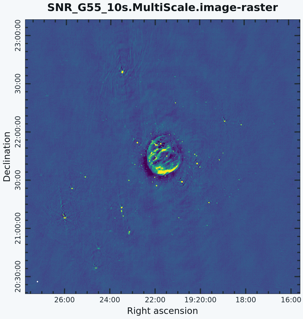
Since G55.7+3.4 is an extended source with many spatial scales, the most basic (yet still reasonable) imaging procedure is to use clean with multiple scales. MS-CLEAN is an extension of the classical CLEAN algorithm for handling extended sources. It works by assuming the sky is composed of emission at different spatial scales and works on them simultaneously, thereby creating a linear combination of images at different spatials scales. For a more detailed description of Multi Scale CLEAN, see the paper by J.T. Cornwell entitled Multi-Scale CLEAN deconvolution of radio synthesis images.

As is suggested, we will use a set of scales (which are expressed in units of the requested pixel, or cell, size) which are representative of the scales that are present in the data, including a zero-scale for point sources.

Note that interrupting clean by Ctrl+C may corrupt your visibilities -- you may be better off choosing to let clean finish. We are currently implementing a command that will nicely exit to prevent this from happening, but for the moment try to avoid Ctrl+C.

G55.7+3.4 Multi-Scale Clean

Artifacts around point sources

# In CASA
clean(vis='SNR_G55_10s.calib.ms', imagename='SNR_G55_10s.MultiScale', 
      imsize=1280, cell='8arcsec', multiscale=[0,6,10,30,60], smallscalebias=0.9, 
      interactive=False, niter=1000,  weighting='briggs', stokes='I', 
      threshold='0.1mJy', usescratch=F, imagermode='csclean')

viewer('SN_G55_10s.MultiScale.image')

• imagename='SN_G55_10s.MultiScale': the root filename used for the various clean outputs. These include the final image (<imagename>.image), the relative sky sensitivity over the field (<imagename>.flux), the point-spread function (also known as the dirty beam; <imagename>.psf), the clean components (<imagename>.model), and the residual image (<imagename>.residual).

• imsize=1280: the image size in number of pixels. Note that entering a single value results in a square image with sides of this value. There are imsize values where clean is not very efficient. The logger should tell you if you hit such a number and suggest a better one. As a rule of thumb, <maths>10*2^n</maths> results ins speedy imsizes.

• cell='8arcsec': the size of one pixel; again, entering a single value will result in a square pixel size.

• multiscale=[0,6,10,30,60]: a set of scales on which to clean. A good rule of thumb when using multiscale is [0, 2xbeam, 5xbeam] (where beam is the synthesized beam) and larger scales up to about half the minor axis maximum scale of the mapped structure. Since these are in units of the pixel size, our chosen values will be multiplied by the requested cell size. Thus, we are requesting scales of 0 (a point source), 48, 80, 240, and 480 arcseconds. Note that 16 arcminutes (960 arcseconds) roughly corresponds to the size of G55.7+3.4.

• smallscalebias=0.9: This parameter is known as the small scale bias, and helps with faint extended structure, by balancing the weight given to smaller structures which tend to be brighter, but have less flux density. Increasing this value gives more weight to smaller scales. A value of 1.0 weighs the largest scale to zero, and a value of less than 0.2 weighs all scales nearly equally. The default value is 0.6.

• interactive=False: we will let clean use the entire field for placing model components. Alternatively, you could try using interactive=True, and create regions to constrain where components will be placed. However, this is a very complex field, and creating a region for every bit of diffuse emission as well as each point source can quickly become tedious. For a tutorial that covers more of an interactive clean, please see IRC+10216 tutorial.

• niter=1000: this controls the number of iterations clean will do in the minor cycle.

• weighting='briggs': use Briggs weighting with a robustness parameter of 0 (halfway between uniform and natural weighting).

• stokes='I': since we have not done any polarization calibration, we only create a total-intensity image.

• threshold='0.1mJy': Flux level at which to stop cleaning.

• usescratch=F: do not write the model visibilities to the model data column (only needed for self-calibration)

• imagermode='csclean': use the Cotton-Schwab clean algorithm

• threshold='0.1mJy': threshold at which the cleaning process will halt; i.e. no clean components with a flux less than this value will be created. This is meant to avoid cleaning what is actually noise (and creating an image with an artificially low rms). It is advisable to set this equal to the expected rms, which can be estimated using the EVLA exposure calculator. However, in our case, this is a bit difficult to do, since we have lost a hard-to-estimate amount of bandwidth due to flagging, and there is also some residual RFI present. Therefore, we choose 0.1 mJy as a relatively conservative limit.

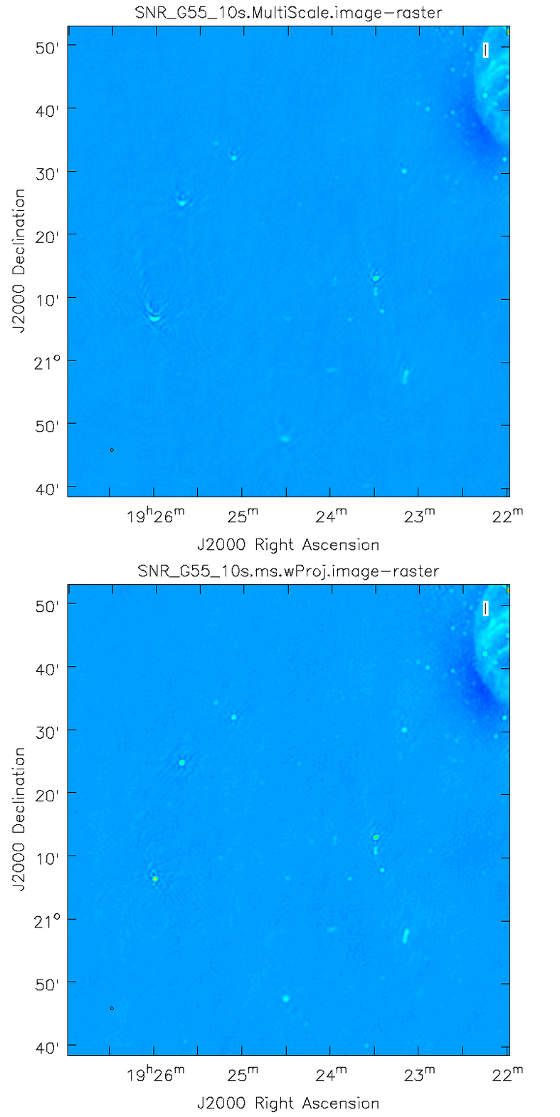
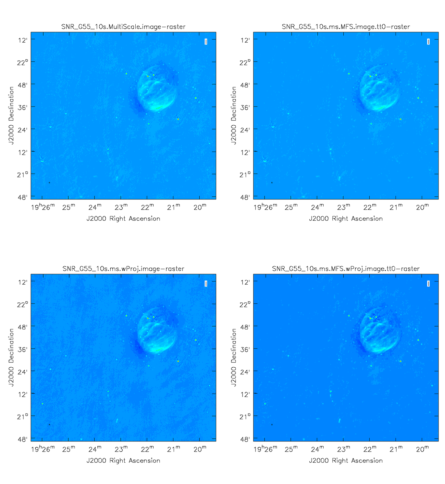
This is the fastest of the imaging techniques described here, but it's easy to see that there are artifacts in the resulting image. Note that you may have to play with the image color map and brightness/contrast to get a better view of the image details. This can be done by clicking on Data Display Options (wrench icon on top left corner), and choosing "rainbow 3" under basic settings. We can use the viewer to explore the point sources near the edge of the field by zooming in on them. Some have prominent arcs, as well as spots in a six-pointed pattern surrounding them.

Next we will explore some more advanced imaging techniques to mitigate the artifacts seen towards the edge of the image.

Multi-Scale, Wide-Field Clean (w-projection)

Faceting when using widefield gridmode, which can be used in conjunction with w-projection.

Multi-Scale image of arcs around point sources far from the phase center, versus MS with w-projection. We can see the that combining the w-projection algorithm with the multiscale algorithm improves the resulting image by removing prominent artifacts.

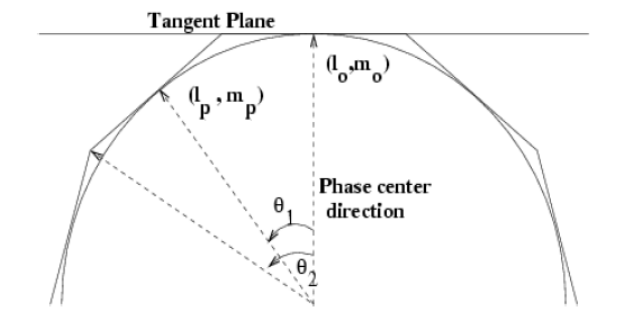
The next clean algorithm we will employ is w-projection, which is a wide-field imaging technique that takes into account the non-coplanarity of the baselines as a function of distance from the phase center. For wide-field imaging, the sky curvature and non-coplanar baselines results in a non-zero w-term. The w-term introduced by the sky and array curvature introduces a phase term that will limit the dynamic range of the resulting image. Applying 2-D imaging to such data will result in artifacts around sources away from the phase center, as we saw in running MS-CLEAN. Note that this affects mostly the lower frequency bands, especially for the more extended configurations, due to the field of view decreasing with higher frequencies.

The w-term can be corrected by faceting (describe the sky curvature by many smaller planes) in either the image or uv-plane, or by employing w-projection. A combination of the two can also be employed within clean by setting the parameter gridmode='widefield'. If w-projection is employed, it will be done for each facet. Note that w-projections is an order of magnitude faster than the faceting algorithm, but will require more memory.

For more details on w-projection, as well as the algorithm itself, see "The Noncoplanar Baselines Effect in Radio Interferometry: The W-Projection Algorithm". Also, the chapter on Imaging with Non-Coplanar Arrays may be helpful.

# In CASA
clean(vis='SNR_G55_10s.calib.ms', imagename='SNR_G55_10s.ms.wProj',
      gridmode='widefield', imsize=1280, cell='8arcsec',
      wprojplanes=128, multiscale=[0,6,10,30,60], 
      interactive=False, niter=1000,  weighting='briggs',
      stokes='I', threshold='0.1mJy', usescratch=F, imagermode='csclean')

viewer('SNR_G55_10s.ms.wProj.image')

• gridmode='widefield': Use the w-projection algorithm.

• wprojplanes=128: The number of w-projection planes to use for deconvolution; 128 is the minimum recommended number.

This will take slightly longer than the previous imaging round; however, the resulting image has noticeably fewer artifacts. In particular, compare the same outlier source in the Multi-Scale w-projected image with the Multi-Scale-only image: note that the swept-back arcs have disappeared. There are still some obvious imaging artifacts remaining, though.

Multi-Scale, Multi-Term Frequency Synthesis

Multi-Frequency Synthesis snapshot of (u,v) coverage. We can see from the image on the right, using this algorithm can greatly improve coverage, thereby improving image fidelity.

Multi-Scale image artifacts versus MS-MFS artifacts near SNR, with nterms=2. We can see artifacts around point sources diminish, improving our image.

Spectral Index image

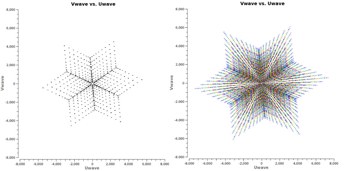
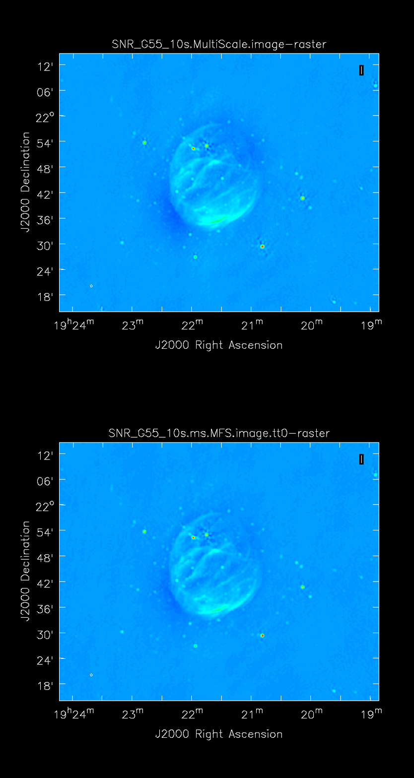
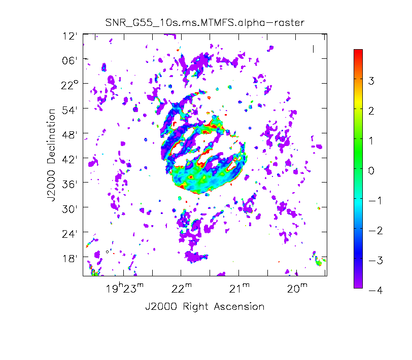
Another consequence of simultaneously imaging the wide fractional bandwidths available with the EVLA is that the primary and synthesized beams have substantial frequency-dependent variation over the observing band. If this is not accounted for, it will lead to imaging artifacts and compromise the achievable image rms.

The dimensions of the (u,v) plane are measured in wavelengths, and therefore observing at several frequencies, a baseline can sample several ellipses in the (u,v) plane, each with different sizes. We can therefore fill in the gaps in the single frequency (u,v) coverage, hence Multi-Frequency Synthesis (MFS). Also when observing in low-frequencies, it may prove beneficial to observe in small time-chunks, which are spread out in time. This will allow the coverage of more spatial-frequencies, allowing us to employ this algorithm more efficiently.

The Multi-Scale Multi-Frequency-Synthesis (MS-MFS) algorithm provides the ability to simultaneously image and fit for the intrinsic source spectrum. The spectrum is approximated using a polynomial Taylor Term expansion in frequency, with the degree of the polynomial as a user-controlled parameter. A least-squares approach is used, along with the standard clean-type iterations. Using this method of imaging will dramatically improve our (u,v) coverage, hence improving image fidelity.

For a more detailed explanation of the MS-MFS deconvolution algorithm, please see the paper by Urvashi Rau and Tim J. Cornwell entitled A multi-scale multi-frequency deconvolution algorithm for synthesis imaging in radio interferometry

# In CASA
clean(vis='SNR_G55_10s.calib.ms', imagename='SNR_G55_10s.ms.MFS',
      imsize=1280, cell='8arcsec', mode='mfs', nterms=2,
      multiscale=[0,6,10,30,60], 
      interactive=False, niter=1000,  weighting='briggs',
      stokes='I', threshold='0.1mJy', usescratch=F, imagermode='csclean')

viewer('SNR_G55_10s.ms.MFS.image.tt0')

viewer('SNR_G55_10s.ms.MFS.image.alpha')

• nterms=2:the number of Taylor terms to be used to model the frequency dependence of the sky emission. Note that the speed of the algorithm will depend on the value used here (more terms will be slower); of course, the image fidelity will improve with a larger number of terms (assuming the sources are sufficiently bright to be modeled more completely).

This will take much longer than the two previous methods, so it would probably be a good time to have coffee or chat about EVLA data reduction with your neighbor at this point.

When clean is done <imagename>.image.tt0 will contain a total intensity image, where tt0 is a suffix to indicate the Taylor term; <imagename>.image.alpha will contain an image of the spectral index in regions where there is sufficient signal-to-noise. Having this spectral index image can help convey information about the emission mechanism involved within the supernova remnant. It can also give information on the optical depth of the source. I've included a color widget on the top of the plot to give an idea of the spectral index variation.

For more information on the multi-frequency synthesis mode and its outputs, see section 5.2.5.1 in the CASA cookbook.

Inspect the brighter point sources in the field near the supernova remnant. You will notice that some of the artifacts which had been symmetric around the sources themselves are now gone; however, since we did not use W-Projection this time, there are still strong features related to the non-coplanar baseline effects still apparent for sources further away.

Multi-Scale, Multi-Term Frequency, Widefield Clean

Finally, we will combine the W-Projection and MS-MFS algorithms to simultaneously account for both of the effects. Be forewarned -- these imaging runs will take a while, and it's best to start them running and then move on to other things.

First, we will image the autoflagged data. Using the same parameters for the individual-algorithm images above, but combined into a single clean run, we have:

Here we see the differences as the images progress through the different algorithms used: MS -> MS-MFS -> MS-wProjection -> MS-MFS-wProjection.

# In CASA
clean(vis='SNR_G55_10s.calib.ms', imagename='SNR_G55_10s.ms.MFS.wProj',
      gridmode='widefield', imsize=1280, cell='8arcsec', mode='mfs',
      nterms=2, wprojplanes=128, multiscale=[0,6,10,30,60],  
      interactive=False, niter=1000,  weighting='briggs',
      stokes='I', threshold='0.1mJy', usescratch=F, imagermode='csclean')

viewer('SNR_G55_10s.ms.MFS.wProj.image.tt0')

viewer('SNR_G55_10s.ms.MFS.wProj.image.alpha')

Again, looking at the same outlier source, we can see that the major sources of error have been removed, although there are still some residual artifacts. One possible source of error is the time-dependent variation of the primary beam; another is the fact that we have only used nterms=2, which may not be sufficient to model the spectra of some of the point sources.

Ultimately, it isn't too surprising that there was still some RFI present in our auto-flagged data, since we were able to see this with plotms. It's also possible that the auto-flagging overflagged some portions of the data, also leading to a reduction in the achievable image rms.

Imaging Outlier Fields

Now we will image the supernova remnant, as well as the bright sources (outliers) towards the edges of the image, creating a 512x512 pixel image for each one. For this, we will be utilizing CLEAN without widefield mode (try it to see the effects) as we will be specifying a phase center, and the images will not be too big, therefore we will not have sources very far from the phase center. We will specify a name for each image, as well as a phase center for each image. This form of imaging is useful for when you have several outlier fields you'd like to image in one go. An outlier file can also be created, if you have a list of sources you'd like to image.

# In CASA
clean(vis='SNR_G55_10s.calib.ms', imagename=['SNR.MS.MFS', 'Outlier1.MS.MFS', 'Outlier2.MS.MFS'],
      imsize=[[512,512],[512,512],[512,512]], cell='8arcsec', mode='mfs',
      multiscale=[0,6,10,30,60], interactive=False, niter=1000,  weighting='briggs',
      stokes='I', threshold='0.1mJy', usescratch=F, imagermode='csclean',
      phasecenter=['J2000 19h21m38.271 21d45m48.288', 'J2000 19h23m27.693 22d37m37.180', 'J2000 19h25m46.888 21d22m03.365'])

Images of the supernova remnant and bright outlying sources.

Primary Beam Correction

In interferomety, the images formed via deconvolution, are representations of the sky, multiplied by the primary beam response of the antenna. The primary beam can be described by a Gaussian with the size depending on the observing frequency. Images produced via CLEAN are not corrected for the primary beam pattern (important for mosaics), and therefore do not have the correct flux. Correcting the primary beam can be done during clean with the pbcor parameter. It can also be done after imaging using the task impbcor for regular data sets, and widebandpbcor for those that use Taylor-term expansion (nterms > 1). A third possibility, is utilizing the task immath to divide the <imagename>.image by the <imagename>.flux images.

Flux corrected images usually don't look pretty, due to the noise at the edges being increased. Flux densities should only be calculated from primary beam corrected images. Let's run the impbcor task to correct our multiscale image.

# In CASA
impbcor(imagename='SNR_G55_10s.MultiScale.image', pbimage='SNR_G55_10s.MultiScale.flux', outfile='SNR_G55_10s.MS.pbcorr.image', mode='divide')

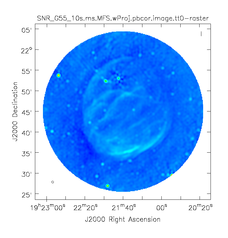
Let us now use the task for widefield images. Note that for this task, we will be supplying the image name that is the prefix for the taylor expansion images, tt0 and tt1, which must be on disk. Such files were created during the last Multi-Scale, Multi-Frequency, Widefield run of CLEAN.

Primary beam corrected image using the MS.MFS.wProj image created during the clean process.

# In CASA
widebandpbcor(vis='SNR_G55_10s.calib.ms', imagename='SNR_G55_10s.ms.MFS.wProj', 
              nterms=2, action='pbcor', pbmin=0.2, spwlist=[0,1,2,3], 
              weightlist=[0.5,1.0,0,1.0], chanlist=[63,63,63,63], threshold='0.1Jy')

• spwlist=[0,1,2,3] : We want to apply this correction to all spectral windows in our calibrated measurement set.
• weightlist=[0.5,1.0,0,1.0] : Since we did not specify rest frequencies during CLEAN, the widbandpbcor tasks will pick them from the provided image. Running the task, the logger reports the multiple frequencies used for the primary beam, which are 1.256, 1.429, 1.602, and 1.775 GHz. Having created an amplitude vs. frequency plot of the calibrated measurement set with colorized spectral windows using plotms, we notice that the first chosen frequency lies within spectral window 0, which we know had lots of flagged data due to lots of RFI being present. This weightlist parameter allows us to give this chosen frequency less weight. The primary beam at 1.6GHz lies in an area with no data, therefore we will give a weight value of zero for this frequency. The remaining frequencies 1.429 and 1.775 GHz lie within spectral windows which contained less RFI, therefore we provide a larger weight percentage.
• pbmin=0.2 : Gain level below which not to compute Taylor-coefficients or apply a primary beam correction.
• chanlist=[63,63,63,63] : Our measurment set contains 64 channels, including zero.
• threshold='0.1Jy' : Threshold in the intensity map, below which not to recalculate the spectral index.

It's important to note that the image will cut off at about 20% of the HPBW, as we are confident of the accuracy within this percentage. Anything outside becomes less accurate, thus there is a mask associated with the creation of the corrected primary beam image.

It would be a good exercise to use viewer to plot both the primary beam corrected image, and the original cleaned image and compare the intensity (Jy/beam) values, which should differ slightly.

Image Information

Frequency Reference Frame

The velocity within your image is calculated based on your choice of frame, velocity definition, and spectral line rest frequency. The initial frequency reference frame is initially given by the telescope, however, it can be transformed to several other frames, including:

• LSRK - Local Standard of Rest Kinematic. Conventional LSR based on average velocity of stars in the solar neighborhood.
• LSRD - Local Standard of Rest Dynamic. Velocity with respect to a frame in circular motion about the galactic center.
• BARY - Barycentric. Referenced to JPL ephemeris DE403. Slightly different and more accurate than heliocentric.
• GEO - Geocentric. Referenced to the Earth's center. This will just remove the observatory motion.
• TOPO - Topocentric. Fixed observing frequency and constantly changing velocity.
• GALACTO - Galactocentric. Referenced to the dynamical center of the galaxy.
• LGROUP - Local Group. Referenced to the mean motion of Local Group of Galaxies.
• CMB - Cosmic Microwave Background dipole. Based on COBE measurements of dipole anisotropy.

Image Header

The image header holds meta data associated with your CASA image. The task imhead will display this data within the casalog. We will first run imhead with mode='summary':

# In CASA
imhead(imagename='SNR_G55_10s.ms.MFS.wProj.image.tt0', mode='summary')

• mode='summary': gives general information about the image, including the object name, sky coordinates, image units, the telescope the data was taken with, and more.

For further information about the image, let's now run it with mode='list':

# In CASA
imhead(imagename='SNR_G55_10s.ms.MFS.wProj.image.tt0', mode='list')

• mode='list': gives more detailed information, including beam major/minor axes, beam primary angle, and the location of the max/min intensity, and lots more.

We will now want to change our image header units from Jy/beam to Kelvin. To do this, we will run the task with mode='put':

# In CASA
imhead(imagename='SNR_G55_10s.ms.MFS.wProj.image.tt0', mode='put', hdkey='bunit', hdvalue='K')

Let's also change the direction reference frame from J2000 to Galactic:

# In CASA
imhead(imagename='SNR_G55_10s.ms.MFS.wProj.image.tt0', mode='put', hdkey='equinox', hdvalue='GALACTIC')

↵ CASAguides

-- Original: Miriam Hartman
-- Modifications: Lorant Sjouwerman (4.4.0, 2015/07/07)
-- Modifications: Jose Salcido (4.5.2, 2016/02/24)
-- Modifications: Juergen Ott (4.5.2, 2016/04/14)

Last checked on CASA Version 4.5.2