3C286 Band6Pol Imaging for CASA 4.3

This page is currently under construction.

DO NOT USE IT.

To navigate the CASAguides pages, visit [http://casaguides.nrao.edu/ casaguides.nrao.edu ]

Overview

This portion of the 3C286_Polarization CASA Guide will cover the imaging of the total power and polarized emission.

In section 2 we will image the data before the D-terms correction, to verify the effect on the images of this correction. To run this imaging you need to have completed the calibration part and have generated all the calibration tables. If you did not complete the Calibration part of the guide, you can skip to next section.

Section 3 begins where the 3C286_Band6Pol_Calibration_for_CASA_4.3 section left off: right after running the CASA task split to split off the science target from the rest of the measurement set following calibration. If you completed the Calibration section of the guide, then you can continue where you left off, with 3c286_SVpol.cal.ms. If you did not complete the Calibration portion of the guide, then you can download the calibrated uvdata by clicking on the region closest to your location:

MODIFY OR DELETE IF NOT NEEDED

North America

Europe

East Asia

Once there, download the file '3C286_Band6_pol_Calibrated.tgz' to obtain the calibrated uvdata.

Once the download has finished, unpack the file:

# In a terminal outside CASA
tar -xvzf 3C286_Band6_pol_Calibrated.tgz

cd 3C286_Band6_pol_Calibrated

# Start CASA
casapy

After that, you should have 3c286_SVpol.cal.ms in your working directory.

Imaging of the polarization calibrator with and without applying D-terms corrections

To verify the actual effect of D-terms correction on the images, we apply to the polarization calibrator all calibration tables computed in the calibration guide except the D-terms corrections.

# In CASA

applycal(vis='3c286_SV.ms', 
         field='0', 
         calwt=F,
         gaintable=['3c286_SV.ms.Bscan','3c286_SV.ms.G2.polcal','3c286_SV.ms.Kcrs', '3c286_SV.ms.XY0'],
         interp=['nearest','linear', 'nearest','nearest'],  
         gainfield=['', '', '','', '', ''],
         parang=T)

Now we make a full-polarization image of the polarization calibrator. Here, just for inspection purposes, we clean non-interactively using the default parameters, which means cleaning the entire image with 500 iterations.

# In CASA

os.system('rm -rf Field0.noDterm.Stokes.clean*')
clean(vis='3c286_SV.ms',
      field='0',
      imagename='Field0.noDterm.Stokes.clean',
      cell=['0.1arcsec'],
      imsize=[250,250],
      stokes='IQUV',
      interactive=F)

In the following section you will find a more clear explanation of how to define the cell and imsize parameters.

Now we apply all the calibration tables, including Df0gen:

# In CASA

applycal(vis='3c286_SV.ms', 
         field='0', 
         calwt=F,
         gaintable=['3c286_SV.ms.Bscan','3c286_SV.ms.G2.polcal','3c286_SV.ms.Kcrs','3c286_SV.ms.XY0','3c286_SV.ms.Df0gen'],
         interp=['nearest','linear', 'linear','nearest', 'nearest'],  
         gainfield=['', '','', '', ''],
         parang=T)

And we clean again:

# In CASA

os.system('rm -rf Field0.withDterm.Stokes.clean*')
clean(vis='3c286_SV.ms',
      field='0',
      imagename='Field0.withDterm.Stokes.clean',
      cell=['0.1arcsec'],
      imsize=[250,250],
      stokes='IQUV',
      interactive=F)

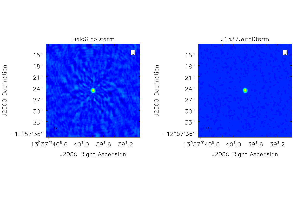
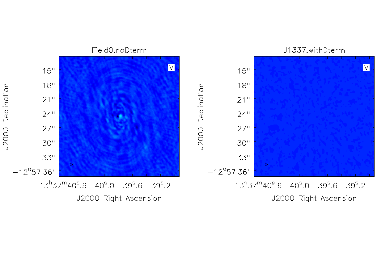
As you can see in <xr id="comparison" />, the application of D-term calibration clearly improves the images of Stokes Q, U, and V.

<figure id="comparison">

• 
  Stokes I.
• 
  Stokes Q.
• 
  Stokes U.
• 
  Stokes V.

<xr id="comparison" nolink/>. Comparison between images of the polarization calibrator without (left panels) and with (right panels) the D-term corrections applied. </figure>

Full polarization imaging of the target

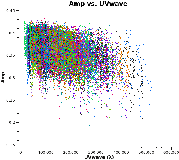
We will start by making a continuum image of 3C286 using clean. Before starting the cleaning, it makes sense to check if the emission is resolved or not by plotting amplitude as a function of uv-distance. The higher amplitudes at shorter uv-distances suggest that the source is slightly resolved.

# In CASA
plotms(vis='3c286_SVpol.cal.ms', spw='', xaxis='uvwave', yaxis='amp', correlation='XX,YY',
       avgtime='1e8', avgchannel='128', coloraxis='baseline')

Amplitude vs. uv-distance. The source seems to be slightly resolved.

This plot also helps us defining the cellsize needed for the task clean. From the plot we see that the longest baseline is 500 kilo wavelength. This means that the maximum resolution can be approximately 1/500000*206265 arcsec = 0.4 arcsec. We will use a cellsize=0.1, to oversample the beam sufficiently. The FWHM of the primary beam of ALMA in Band 6 is about 25 arcsec, and we want to image out to at least that extent, so we will use imsize=250.

# In CASA
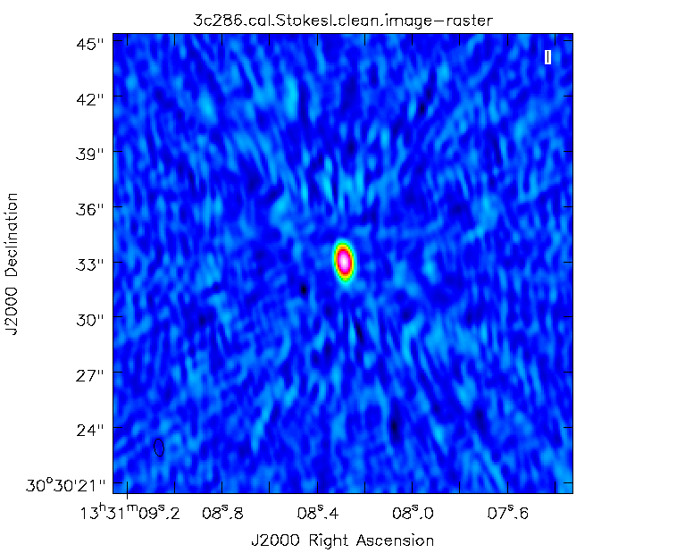
os.system('rm -rf 3c286.cal.StokesI.clean*')
clean(vis='3c286_SVpol.cal.ms',
      imagename='3c286.cal.StokesI.clean',
      cell=['0.1arcsec'],
      imsize=[250,250],
      stokes='I',
      interactive=F)

Here, we use the non-interactive mode, specifying interactive=F. In the interactive mode (interactive=T), the clean task will bring up a viewer where clean regions can be defined, see Antennae casaguide for further details on the interactive use of clean.

Finally, note that we delete any previous versions of the output images before proceeding with the clean command. This is important, because if images with the supplied root name already exist, CASA will clean those further instead of producing new output images.

After the imaging and deconvolution process has finished, you can use the viewer to look at your image.

# In CASA
viewer('3c286.cal.StokesI.clean.image')

Total intensity image of 3C286

We will determine some statistics for the image using the task imstat (some details are given below):

# In CASA
calstat=imstat(imagename='3c286.cal.StokesI.clean.image', region='', box='10,10,90,35')
rms=(calstat['rms'][0])
print '>> rms in continuum image: '+str(rms)
calstat=imstat(imagename='3c286.cal.StokesI.clean.image', region='')
peak=(calstat['max'][0])
print '>> Peak in continuum image: '+str(peak)
print '>> Dynamic range in continuum image: '+str(peak/rms)

This tells us that the rms of this image is 1.1 mJy and the peak flux density is ~337 mJy. The dynamic range (ratio between peak and rms) is approximately 300.

For future reference, we create a png file of the continuum image:

# In CASA
os.system('rm -rf 3c286.cal.StokesI.clean.png')
imview(raster={'file': '3c286.cal.StokesI.clean.image', 'colorwedge':T,
               'range':[-0.006, 0.4], 'scaling':-0.4, 'colormap':'Rainbow 2'},
        out='3c286.cal.StokesI.clean.png', zoom=2)

We now use the same tasks to obtain the stokes Q,U, and V images separately. There is also the possibility to obtain a four-channels image containing all the Stokes IQUV; however, since we will need each image separately when we construct the polarization images, we make all of them separately. Is this the only reason why we don't use the stokes='IQUV'?

# In CASA
os.system('rm -rf 3c286.cal.StokesQ.clean*')
clean(vis='3c286_SVpol.cal.ms',
      imagename='3c286.cal.StokesQ.clean',
      cell=['0.1arcsec'],
      imsize=[250,250],
      stokes='Q',
      interactive=T)
calstat=imstat(imagename='3c286.cal.StokesQ.clean.image', region='', box='10,10,90,35')
rms=(calstat['rms'][0])
print '>> rms in continuum image: '+str(rms)
calstat=imstat(imagename='3c286.cal.StokesQ.clean.image', region='')
peak=(calstat['max'][0])
print '>> Peak in continuum image: '+str(peak)
print '>> Dynamic range in continuum image: '+str(peak/rms)

# In CASA
os.system('rm -rf 3c286.cal.StokesU.clean*')
clean(vis='3c286_SVpol.cal.ms',
      imagename='3c286.cal.StokesU.clean',
      cell=['0.1arcsec'],
      imsize=[250,250],
      stokes='U',
      interactive=T)
calstat=imstat(imagename='3c286.cal.StokesU.clean.image', region='', box='10,10,90,35')
rms=(calstat['rms'][0])
print '>> rms in continuum image: '+str(rms)
calstat=imstat(imagename='3c286.cal.StokesU.clean.image', region='')
peak=(calstat['max'][0])
print '>> Peak in continuum image: '+str(peak)
print '>> Dynamic range in continuum image: '+str(peak/rms)

# In CASA
os.system('rm -rf 3c286.cal.StokesV.clean*')
clean(vis='3c286_SVpol.cal.ms',
      imagename='3c286.cal.StokesV.clean',
      cell=['0.1arcsec'],
      imsize=[250,250],
      stokes='V',
      interactive=T)
calstat=imstat(imagename='3c286.cal.StokesV.clean.image', region='', box='10,10,90,35')
rms=(calstat['rms'][0])
print '>> rms in continuum image: '+str(rms)
calstat=imstat(imagename='3c286.cal.StokesV.clean.image', region='')
peak=(calstat['max'][0])
print '>> Peak in continuum image: '+str(peak)
print '>> Dynamic range in continuum image: '+str(peak/rms)

The results of the measurements for the I, Q, and U images are reported in the table below. All flux densities are reported in mJy/beam.

	I	Q	U
rms	1.1	0.05	0.1
Peak	337	12.4	54
Dyn range	300	254	298

Constructing Polarization Intensity and Angle Images

We have now produced the images for all the four Stokes parameters: I, Q, U, and V. Stokes Q and U describe the linear polarization and V describes the circular polarization. Specifically, Q describes the amount of linear polarization aligned with a given axis, and U describes the amount of linear polarization at a 45 deg angle to that axis. The V parameter describes the amount of circular polarization, with the sign (positive or negative) describing the sense of the circular polarization (right- or left-hand circularly polarized).

In general, few celestial sources are expected to show circular polarization, with the notable exception of masers. Terrestrial and satellite sources are often highly circularly polarized. The V image is therefore often worth forming because any V emission could be indicative of unflagged RFI within the data (or problems with the calibration!).

Because the Q and U images both describe the amount of linear polarization, it is more common to work with a linear polarization intensity image, [math]\displaystyle{ P = \sqrt{Q^2 +U^2} }[/math]. We can also calculate the polarization position angle [math]\displaystyle{ \chi = 0.5 arctan U/Q }[/math].

The relevant task is immath; for specific examples of polarization image processing see Polarization Manipulation.

To form the linear polarization image, we combine the Q and U images using the mode='poli' option of immath.

# In CASA
os.system('rm -rf 3c286_SV.POLI')
immath(outfile='3c286_SV.POLI',
       mode='poli',
       imagename=['3c286.cal.StokesQ.clean.image','3c286.cal.StokesU.clean.image'],
       sigma='0.0Jy/beam')

# In CASA
calstat=imstat(imagename='3c286_SV.POLI', region='', box='10,10,90,35')
rms=(calstat['rms'][0])

The measured rms is 0.15 mJy/beam.

To form the polarization position angle image we combine again the Q and U images using the mode='pola' option of immath. The Q and U images can be listed in either order. To avoid displaying the position angle of noise, we can use the polithresh parameter to set a threshold intensity of the linear polarization above which we wish to calculate the polarization angle. An appropriate level here might be the 5σ level of the polarization image, about 1 mJy/beam.

# In CASA
os.system('rm -rf 3c286_SV.POLA')
immath(outfile='3c286_SV.POLA',
       mode='pola',
       imagename=['3c286.cal.StokesQ.clean.image','3c286.cal.StokesU.clean.image'],
       polithresh='0.5mJy/beam')

If desired, it is also possible to form the fractional linear polarization image, defined as P/I.

# In CASA
os.system('rm -rf 3c286_SV.RATIO')
immath(outfile='3c286_SV.RATIO',
       mode='evalexpr',
       imagename=['3c286.cal.StokesI.clean.image','3c286.cal.StokesQ.clean.image','3c286.cal.StokesU.clean.image'],
       expr='sqrt((IM1^2+IM2^2)/IM0[IM0>5e-3]^2)')

Since the total intensity image can (and hopefully does) approach zero in regions free of source emission, dividing by the total intensity can produce very high pixel values in these regions. We therefore wish to restrict our fractional polarization image to regions containing real emission, which we do by setting a threshold in the total intensity image, which in this case corresponds to five times the noise level in the Stokes I image. The computation of the polarized intensity is specified in the previous command by

       expr='sqrt((IM1^2+IM2^2)/IM0[IM0>5e-3]^2)'

with the expression in square brackets setting the threshold in IM0 (the total intensity image). Note that IM0, IM1 and IM2 correspond to the three files listed in the imagename array, in that order. In this case, the order in which the different images are specified is critical.

Image visualization and analysis

Now we can view these various images using viewer. It is instructive to display the I, P, and [math]\displaystyle{ \chi }[/math] images (total intensity, total linearly polarized intensity, and polarization position angle) together, to show how the polarized emission relates to the total intensity, and how the magnetic field is structured. We can do this using the viewer.

• Begin by loading the linear polarization image in the viewer:

# In CASA
viewer('3c286_SV.POLI')

• Next, load the total intensity image as a contour image. In the viewer panel, hit the "Open" icon (the leftmost button in the top row of icons in the viewer). This will bring up a 'Load Data' GUI showing all images and MS in the current directory. Select the total intensity image (3c286.cal.StokesI.clean.image) and click the 'Contour Map' button on the right hand side.
• Finally, load the polarization position angle image (3c286_SV.POLA) as a vector map.

File:Three images.png

Full-polarization image of 3C286

While we set the polithresh parameter when we created the position angle ([math]\displaystyle{ \chi }[/math]) image, a digression here is instructive in the use of LEL Expressions. Had we not set this parameter, the position angle would have been derived for all pixels within the full IQUV image cube. There is only polarized emission from a limited subset of pixels within this image. Therefore, to avoid plotting vectors corresponding to the position angle of pure noise, we now wish to select only the regions where the polarized intensity is brighter than some threshold value. To do this, we use an LEL (Lattice Expression Language) Expression in the 'Load Data' GUI. For our chosen threshold of 0.4 mJy/beam (the 5 sigma level in the P image), we paste the expression

     '3c286_SV.POLA'['3c286_SV.POLI'>0.001]

into the LEL Expression box in the GUI, and click the 'Vector Map' button. This would load the vectors only for regions where P>1 mJy/beam.

To optimize the display for ease of interpretation we click the wrench icon to open a 'Data Display Options' GUI. This will have 3 tabs, corresponding to the three images loaded. We can change the image color map and transfer function, the contour levels and color, and the the vector spacing and color.

For the polarization angle vector it is also possible to add a rotation. The polarization position angle as calculated is the electric vector position angle (EVPA). If we are interested in the orientation of the magnetic field, then for an optically thin source the magnetic field orientation is perpendicular to the EVPA, so we must rotate the vectors by 90 degrees. Select the vector image tab in the 'Data Display Options' GUI (labeled as the LEL expression we entered in the Load Data GUI) and enter 90 in the Extra rotation box. If the vectors appear too densely packed on the image, change the spacing of the vectors by setting X-increment and Y-increment to a larger value.

To get quantitative information from the images, we can either use the task imstat (we already used it above) or the task imfit. The task imstat returns the statistics in a Python dictionary, from which we can read what we need in a Python variable. In this example we extract the peak value:

CASA<1> calstat=imstat(imagename='3c286_SV.POLI', region='')

CASA<2> calstat
  Out[1]: 
{'blc': array([0, 0, 0, 0], dtype=int32),
 'blcf': '13:31:09.255, +30.30.20.460, Plinear, 2.33e+11Hz',
 'flux': array([ 0.2630017]),
 'max': array([ 0.0555443]),
 'maxpos': array([125, 125,   0,   0], dtype=int32),
 'maxposf': '13:31:08.288, +30.30.32.960, Plinear, 2.33e+11Hz',
 'mean': array([ 0.00020777]),
 'medabsdevmed': array([  7.20023963e-05]),
 'median': array([ 0.00012894]),
 'min': array([  1.35889238e-07]),
 'minpos': array([213, 165,   0,   0], dtype=int32),
 'minposf': '13:31:07.607, +30.30.36.960, Plinear, 2.33e+11Hz',
 'npts': array([ 62500.]),
 'quartile': array([ 0.00015494]),
 'rms': array([ 0.0011654]),
 'sigma': array([ 0.00114674]),
 'sum': array([ 12.9854018]),
 'sumsq': array([ 0.08488477]),
 'trc': array([249, 249,   0,   0], dtype=int32),
 'trcf': '13:31:07.329, +30.30.45.360, Plinear, 2.33e+11Hz'}

CASA <2>: calstat['max'][0]                                   
  Out[2]: 0.055544301867485046

The task imfit finds one or more elliptical gaussian components on an image region.

# In CASA
fit_res=imfit(imagename='3c286_SV.POLI', region='')

CASA <3>: fit_res
  Out[3]: 
{'converged': array([ True], dtype=bool),
 'results': {'component0': {'flux': {'error': array([ 0.00022216,  0.        ,  0.        ,  0.        ]),
                                     'polarisation': 'Stokes',
                                     'unit': 'Jy',
                                     'value': array([ 0.05968412,  0.        ,  0.        ,  0.        ])},
                            'label': '',
                            'shape': {'direction': {'error': {'latitude': {'unit': 'arcsec',
                                                                           'value': 0.0016846894791978408},
                                                              'longitude': {'unit': 'arcsec',
                                                                            'value': 0.000897955311817972}},
                                                    'm0': {'unit': 'rad',
                                                           'value': -2.7439276172868836},
                                                    'm1': {'unit': 'rad',
                                                           'value': 0.5324854010189068},
                                                    'refer': 'J2000',
                                                    'type': 'direction'},
                                      'majoraxis': {'unit': 'arcsec',
                                                    'value': 0.9247086245361037},
                                      'majoraxiserror': {'unit': 'arcsec',
                                                         'value': 0.0017903156123008801},
                                      'minoraxis': {'unit': 'arcsec',
                                                    'value': 0.5041873260724541},
                                      'minoraxiserror': {'unit': 'arcsec',
                                                         'value': 0.0033723551921053243},
                                      'positionangle': {'unit': 'deg',
                                                        'value': 2.6074689635548425},
                                      'positionangleerror': {'unit': 'deg',
                                                             'value': 0.0643987925372565},
                                      'type': 'Gaussian'},
                            'spectrum': {'frequency': {'m0': {'unit': 'GHz',
                                                              'value': 233.00006749832858},
                                                       'refer': 'LSRK',
                                                       'type': 'frequency'},
                                         'type': 'Constant'}},
             'nelements': 1}}

To extract the flux and its error, we can read them from CASA in Python variables:

# In CASA
fluxPI=fit_res['results']['component0']['flux']['value'][0]
errorPI=fit_res['results']['component0']['flux']['error'][0]

The flux measured in the fitted gaussian is 59.7 mJy with an error of 0.2 mJy.

We now use this method to estimate the fluxes in all the Stokes images:

# In CASA

# First we run imfit 
resI=imfit(imagename = '3c286.cal.StokesI.clean.image', box = '110,110,145,145')
resQ=imfit(imagename = '3c286.cal.StokesQ.clean.image', box = '110,110,145,145')
resU=imfit(imagename = '3c286.cal.StokesU.clean.image', box = '110,110,145,145')
resV=imfit(imagename = '3c286.cal.StokesV.clean.image', box = '110,110,145,145')
 
# and then we extract the flux and error values for each Stokes

fluxI=resI['results']['component0']['flux']['value'][0]
errorI=resI['results']['component0']['flux']['error'][0]

fluxQ=resQ['results']['component0']['flux']['value'][1]
errorQ=resQ['results']['component0']['flux']['error'][1]

fluxU=resU['results']['component0']['flux']['value'][2]
errorU=resU['results']['component0']['flux']['error'][2]
 
fluxV=resV['results']['component0']['flux']['value'][3]
errorV=resV['results']['component0']['flux']['error'][3]

Now we use these values to compute polarization intensity, angle and ratio, and their errors:

# In CASA 
fluxPI  = sqrt( fluxQ**2 + fluxU**2 )
errorPI = sqrt( (fluxQ*errorU)**2 + (fluxU*errorQ)**2 ) / fluxPI

fluxPImjy = 1000*fluxPI
errPImjy  = 1000*errorPI

polRatio = fluxPI / fluxI
errPRat  = polRatio * sqrt( (errorPI/fluxPI)**2 + (errorI/fluxI)**2 )
  
polAngle = 0.5 * degrees( atan2(fluxU,fluxQ) )
errPA    = 0.5 * degrees( errorPI / fluxPI )

The results are collected in the following table:

	Flux	err
I	363 mJy	1.1 mJy
Q	13.42 mJy	0.05 mJy
U	58.1 mJy	0.2 mJy
V	0.0	0.04 mJy
Pol int	59.7 mJy	0.2 mJy
Pol ratio	0.16	0.07
Pol angle	38.5 deg	0.03 deg

As you can see, the polarization intensity computed from the Q and U fluxes is the same as the one extracted from the polarization image (as it should be!).