M100 Band3 Combine 4.3: Difference between revisions
No edit summary |
No edit summary |
||
| Line 38: | Line 38: | ||
= Combine and Image the 7m+12m Interferometric Data = | = Combine and Image the 7m+12m Interferometric Data = | ||
== Split off CO spws == | |||
<source lang="python"> | |||
# In CASA | |||
os.system('rm -rf m100_*m.ms.listobs') | |||
listobs('M100_Band3_12m_CalibratedData.ms',listfile='m100_12m.ms.listobs') | |||
listobs('M100_Band3_7m_CalibratedData.ms',listfile='m100_7m.ms.listobs') | |||
</source> | |||
Below are the observation and spectral window tables from the listobs. | |||
<pre style="background-color: #fffacd;"> | |||
12m data: | |||
ObservationID = 0 ArrayID = 0 | |||
Date Timerange (UTC) Scan FldId FieldName nRows SpwIds Average Interval(s) | |||
10-Sep-2011/18:28:43.4 - 18:41:00.4 11 1 M100 1320 [0, 1, 2, 3] [6.05, 6.05, 6.05, 6.05] | |||
Spectral Windows: (4 unique spectral windows and 1 unique polarization setups) | |||
SpwID Name #Chans Frame Ch1(MHz) ChanWid(kHz) TotBW(kHz) BBC Num Corrs | |||
0 3840 TOPO 113726.419 488.281 1875000.0 1 XX YY | |||
1 3840 TOPO 111851.419 488.281 1875000.0 2 XX YY | |||
2 3840 TOPO 103663.431 -488.281 1875000.0 3 XX YY | |||
3 3840 TOPO 101850.931 -488.281 1875000.0 4 XX YY | |||
7m data: | |||
ObservationID = 0 ArrayID = 0 | |||
Date Timerange (UTC) Scan FldId FieldName nRows SpwIds Average Interval(s) | |||
17-Mar-2013/04:44:04.3 - 04:50:43.7 11 1 M100 168 [0, 1] [10.1, 10.1] | |||
Spectral Windows: (4 unique spectral windows and 1 unique polarization setups) | |||
SpwID Name #Chans Frame Ch1(MHz) ChanWid(kHz) TotBW(kHz) BBC Num Corrs | |||
0 ALMA_RB_03#BB_3#SW-01#FULL_RES 4080 TOPO 111811.300 488.281 1992187.5 3 XX YY | |||
1 ALMA_RB_03#BB_4#SW-01#FULL_RES 4080 TOPO 113686.300 488.281 1992187.5 4 XX YY | |||
2 ALMA_RB_03#BB_1#SW-01#FULL_RES 4080 TOPO 111798.250 488.281 1992187.5 1 XX YY | |||
3 ALMA_RB_03#BB_2#SW-01#FULL_RES 4080 TOPO 113673.250 488.281 1992187.5 2 XX YY | |||
</pre> | |||
<figure id="12m_mosaic.png"> | |||
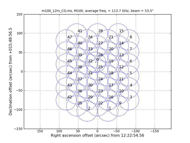
[[Image:12m_mosaic.png|300px|thumb|right|<caption>FOV of 12m mosaic.</caption>]] | |||
</figure> | |||
<figure id="7m_mosaic.png"> | |||
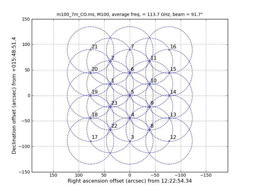
[[Image:7m_mosaic.png|300px|thumb|right|<caption>FOV of 7m mosaic.</caption>]] | |||
</figure> | |||
Examination of the listobs files shows that the CO is in spw=0 for the 12m data and in spws='1,3' for the 7m data. There are two spws containing CO for the 7m data because some of the data was taken with a slightly different correlator setup. | |||
Also note that the integration time per visibility (average interval parameter in listobs) is different: | |||
6.05s for the 12m data and 10.1s for the 7m. This will be important to know later in order to correctly weight the combined data. | |||
Next we split out the CO spectral windows. | |||
<source lang="python"> | |||
# In CASA | |||
os.system('rm -rf m100_12m_CO.ms') | |||
split(vis='M100_Band3_12m_CalibratedData.ms', | |||
outputvis='m100_12m_CO.ms',spw='0',field='M100', | |||
datacolumn='data',keepflags=False) | |||
os.system('rm -rf m100_7m_CO.ms') | |||
split(vis='M100_Band3_7m_CalibratedData.ms', | |||
outputvis='m100_7m_CO.ms',spw='1,3',field='M100', | |||
datacolumn='data',keepflags=False) | |||
</source> | |||
Also of interest is that the 12m data has 48 fields and the 7m has 24 fields (not shown in the excerpt above). The difference in number of pointings is because the 7m antennas have a FWHP (full width half power) primary beam diameter that is 12/7 times larger than the 12m antennas. '''One easy way to see how the mosaics compare is to install the AnalysisUtils package (see [[Analysis_Utilities]])'''. Then with AnalysisUtils you can make the following plots (look at the listobs to obtain the sourceid): | |||
<source lang="python"> | |||
# In CASA | |||
os.system('rm -rf *m_mosaic.png') | |||
au.plotMosaic('m100_12m_CO.ms',sourceid='0',figfile='12m_mosaic.png') | |||
au.plotMosaic('m100_7m_CO.ms',sourceid='1',figfile='7m_mosaic.png') | |||
</source> | |||
We see that the mosaics cover a common area but that the 7m mosaic is a bit larger. This means that the outer edges of the combined mosaic will be noisier than expected if they overlapped perfectly. Just something to look out for. If you had the case where the mosaic coverage is dramatically different, it would be best to exclude the completely non-overlapping fields from the combination. | |||
NOTE: At this stage one would typically do continuum subtraction (if there is any). However we already know from the individual data reductions that the 3mm continuum emission is quite weak and does not significantly contribute to a 5km/s channel, so we will forgo the the continuum subtraction step. Examples of how to do this if you are so inclined are located in the 7m guide and 12m script, respectively. | |||
Revision as of 23:08, 12 January 2015
This page is currently under construction.
DO NOT USE IT.
To navigate the CASAguides pages, visit [http://casaguides.nrao.edu/ casaguides.nrao.edu ]
Overview
This guide describes how to combine the 7m and 12m interferometric data and then how to feather the resulting image with the total power TP image. All of the data for this SV project can be found at https://almascience.nrao.edu/alma-data/science-verification. In order to run this guide you will need to:
- Either run the 7m calibration scripts to obtain the final 7m fully calibrated data or download the fully calibrated data: (i.e. M100_Band3_7m_CalibratedData.tgz)
- Either download the new RawUnCalibrated data for the 12m-array and run the new calibration script or download the fully calibrated data (i.e. M100_Band3_12m_CalibratedData.tgz). Note that while these are the same data that were released previously, the data reduction path has been updated to current best practices and starts from the raw data files called ASDMs (ALMA Science Data Model). Do not use the previously released uncalibrated or calibrated data.
- Either run the M100_Band3_SingleDish_4.3 guide to calibrate and image the Total Power data or download the final image (i.e. M100_TP_Image.tgz)
Confirm your version of CASA
This guide has been written for CASA release 4.3. Please confirm your version before proceeding.
# In CASA
version = casadef.casa_version
print "You are using " + version
if (version < '4.3'):
    print "YOUR VERSION OF CASA IS TOO OLD FOR THIS GUIDE."
    print "PLEASE UPDATE IT BEFORE PROCEEDING."
else:
    print "Your version of CASA is appropriate for this guide."
Combine and Image the 7m+12m Interferometric Data
Split off CO spws
# In CASA
os.system('rm -rf m100_*m.ms.listobs')
listobs('M100_Band3_12m_CalibratedData.ms',listfile='m100_12m.ms.listobs')
listobs('M100_Band3_7m_CalibratedData.ms',listfile='m100_7m.ms.listobs')
Below are the observation and spectral window tables from the listobs.
12m data:

ObservationID = 0         ArrayID = 0
  Date        Timerange (UTC)          Scan  FldId FieldName             nRows     SpwIds   Average Interval(s)
  10-Sep-2011/18:28:43.4 - 18:41:00.4    11      1 M100                      1320  [0, 1, 2, 3]  [6.05, 6.05, 6.05, 6.05]

Spectral Windows:  (4 unique spectral windows and 1 unique polarization setups)
  SpwID  Name   #Chans   Frame   Ch1(MHz)  ChanWid(kHz)  TotBW(kHz) BBC Num  Corrs
  0              3840   TOPO  113726.419       488.281   1875000.0       1  XX  YY
  1              3840   TOPO  111851.419       488.281   1875000.0       2  XX  YY
  2              3840   TOPO  103663.431      -488.281   1875000.0       3  XX  YY
  3              3840   TOPO  101850.931      -488.281   1875000.0       4  XX  YY

7m data:

ObservationID = 0         ArrayID = 0
  Date        Timerange (UTC)          Scan  FldId FieldName             nRows     SpwIds   Average Interval(s)
  17-Mar-2013/04:44:04.3 - 04:50:43.7    11      1 M100                       168  [0, 1]  [10.1, 10.1]

Spectral Windows:  (4 unique spectral windows and 1 unique polarization setups)
  SpwID  Name                           #Chans   Frame   Ch1(MHz)  ChanWid(kHz)  TotBW(kHz) BBC Num  Corrs
  0      ALMA_RB_03#BB_3#SW-01#FULL_RES   4080   TOPO  111811.300       488.281   1992187.5       3  XX  YY
  1      ALMA_RB_03#BB_4#SW-01#FULL_RES   4080   TOPO  113686.300       488.281   1992187.5       4  XX  YY
  2      ALMA_RB_03#BB_1#SW-01#FULL_RES   4080   TOPO  111798.250       488.281   1992187.5       1  XX  YY
  3      ALMA_RB_03#BB_2#SW-01#FULL_RES   4080   TOPO  113673.250       488.281   1992187.5       2  XX  YY
<figure id="12m_mosaic.png">

</figure>
<figure id="7m_mosaic.png">

</figure>
Examination of the listobs files shows that the CO is in spw=0 for the 12m data and in spws='1,3' for the 7m data. There are two spws containing CO for the 7m data because some of the data was taken with a slightly different correlator setup.
Also note that the integration time per visibility (average interval parameter in listobs) is different: 6.05s for the 12m data and 10.1s for the 7m. This will be important to know later in order to correctly weight the combined data.
Next we split out the CO spectral windows.
# In CASA
os.system('rm -rf m100_12m_CO.ms')
split(vis='M100_Band3_12m_CalibratedData.ms',
      outputvis='m100_12m_CO.ms',spw='0',field='M100',
      datacolumn='data',keepflags=False)
os.system('rm -rf m100_7m_CO.ms')
split(vis='M100_Band3_7m_CalibratedData.ms',
      outputvis='m100_7m_CO.ms',spw='1,3',field='M100',
      datacolumn='data',keepflags=False)
Also of interest is that the 12m data has 48 fields and the 7m has 24 fields (not shown in the excerpt above). The difference in number of pointings is because the 7m antennas have a FWHP (full width half power) primary beam diameter that is 12/7 times larger than the 12m antennas. One easy way to see how the mosaics compare is to install the AnalysisUtils package (see Analysis_Utilities). Then with AnalysisUtils you can make the following plots (look at the listobs to obtain the sourceid):
# In CASA
os.system('rm -rf *m_mosaic.png')
au.plotMosaic('m100_12m_CO.ms',sourceid='0',figfile='12m_mosaic.png')
au.plotMosaic('m100_7m_CO.ms',sourceid='1',figfile='7m_mosaic.png')
We see that the mosaics cover a common area but that the 7m mosaic is a bit larger. This means that the outer edges of the combined mosaic will be noisier than expected if they overlapped perfectly. Just something to look out for. If you had the case where the mosaic coverage is dramatically different, it would be best to exclude the completely non-overlapping fields from the combination.
NOTE: At this stage one would typically do continuum subtraction (if there is any). However we already know from the individual data reductions that the 3mm continuum emission is quite weak and does not significantly contribute to a 5km/s channel, so we will forgo the the continuum subtraction step. Examples of how to do this if you are so inclined are located in the 7m guide and 12m script, respectively.