Simalma v2: Difference between revisions
Created page with "Category: Simulations To create a script of the Python code on this page see Extracting scripts from these tutorials. __NOTOC__ == The simalma task == ALMA consists ..." |
No edit summary |
||
| Line 1: | Line 1: | ||
[[Category: Simulations]] | [[Category: Simulations]] | ||
To create a script of the Python code on this page see [[Extracting scripts from these tutorials]]. | To learn how to create a script of the Python code on this page see [[Extracting scripts from these tutorials]]. | ||
__NOTOC__ | __NOTOC__ | ||
== | == Simulations of Observations with the Main 12m Array and the ACA == | ||
ALMA consists of the main array of 12m antennas, the ALMA Compact Array of 7m antennas, and a separate set of 12m antennas used for Total Power measurements. One can simulate observations using any or all of these in CASA. | |||
One could simulate observations that use the main array as well as the ACA by generating the data for each component separately and then "manually" combining and imaging the data. Use '''simobserve''' to generate simulated observations for each component separately, and then combine the Measurement Sets using '''simanalyze'''. This technique is general and can be used to simulate observations using multiple 12m array configurations, as well. Total power observations can be simulated either in an independent run of '''simobserve''', or integrated with one of the interferometric simulations. Note that if you simulate total power and an interferometric observation simultaneously with simobserve, they must have the same set of pointing centers and the same integration and total time. This is probably not realistic. For example, to reduce edge effects, the Total Power antennas should observe a larger area on the sky than the main array antennas, by about 1/2 of a primary beam. So, it is generally better to generate the total power data with a separate run of '''simobserve'''. | |||
This "manual" method of combining main-array data with ACA data is described in the [[ACA_Simulation_(CASA_4.1)]] guide. | |||
== The simalma task == | |||
New in 4.1 is the '''simalma''' task, which takes one set of parameters describing the region of the sky to observe, and makes the appropriate calls to '''simobserve''' and '''simanalyze''' | New in CASA version 4.1 is the '''simalma''' task, which takes one set of parameters describing the region of the sky to observe, and makes the appropriate calls to '''simobserve''' and '''simanalyze'''. Here we give an example showing how to use '''simalma'''. | ||
<font color="purple">As of | <font color="purple">As of July 2013, ALMA is still optimizing the algorithms for combining total power and interferometric data, so the sample parameters used here are likely to change as recommended observing strategies evolve.</font> | ||
| Line 21: | Line 23: | ||
# Set simalma to default parameters | # Set simalma to default parameters | ||
default("simalma") | default("simalma") | ||
# Our project name will be m51, and all simulation products will be placed in a subdirectory m51/ | # Our project name will be "m51", and all simulation products will be placed in a subdirectory "m51/" | ||
project="m51" | project="m51" | ||
</source> | </source> | ||
=====Specify sky model image===== | =====Specify sky model image===== | ||
In this example, we'll use an Halpha image of M51 as the model of the sky. The ''curl'' command used below will copy a data file with the model image to our local disk and rename it. | |||
<source lang="python"> | <source lang="python"> | ||
| Line 36: | Line 38: | ||
Note that '''simalma''' will not modify your original input image. Rather, it will make a copy ''m51/m51.skymodel''. | Note that '''simalma''' will not modify your original input image. Rather, it will make a copy ''m51/m51.skymodel''. | ||
To make the M51 Halpha image more suitable to a sub-millimeter ALMA observation, we will respecify most of the header parameters from the FITS file. We will: | |||
* place the source in the southern hemisphere with the ''indirection'' parameter, | * place the source in the southern hemisphere with the ''indirection'' parameter, | ||
* set the pixel size to 0.1arcsec, to simulate an observation of a galaxy that is smaller in angular size. (M51 itself would require a quite large mosaic, and in any case we'd like the input model pixels to be significantly smaller than the synthesized beam.) | * set the pixel size to 0.1arcsec, to simulate an observation of a galaxy that is smaller in angular size. (M51 itself would require a quite large mosaic, and in any case we'd like the input model pixels to be significantly smaller than the synthesized beam.) | ||
* set the peak brightness to 0.004 Jy/pixel | * set the peak brightness to 0.004 Jy/pixel | ||
* set the frequency to 330GHz, and since it's a 2D image we'll set the single "channel" width to be 50MHz | * set the center observing frequency to 330GHz, and since it's a 2D image we'll set the single "channel" width to be 50MHz. These parameters are plausible for observing a sub-mm emission line in a galaxy. | ||
<source lang="python"> | <source lang="python"> | ||
# Set model image parameters: | # Set model image parameters: | ||
| Line 55: | Line 57: | ||
[[Image:M51.alma_cycle1_3.skymodel.png|thumb|hexagonal mosaic overplotted on sky model]] | [[Image:M51.alma_cycle1_3.skymodel.png|thumb|hexagonal mosaic overplotted on sky model]] | ||
We will simulate observations using the main array in "configuration number 3" from Cycle 1. This configuration affords ~0.5 arcsec resolution. | |||
<source lang="python"> | <source lang="python"> | ||
antennalist="alma_cycle1_3.cfg" | antennalist="alma_cycle1_3.cfg" | ||
</source> | </source> | ||
We'll | We'll set the 12m array observing time to 2 hours: | ||
<source lang="python"> | <source lang="python"> | ||
totaltime="7800s" | totaltime="7800s" | ||
</source> | </source> | ||
Following the Cycle 1 convention, <tt>simalma</tt> | Following the Cycle 1 convention, we will instruct <tt>simalma</tt> to observe 3 times longer with the 7m array and total power dishes. | ||
<source lang="python"> | <source lang="python"> | ||
acaratio=3.0 | acaratio=3.0 | ||
| Line 71: | Line 73: | ||
</source> | </source> | ||
We set the precipitable water vapor to 0.6 mm to represent observations in nominal weather. The simulation will add noise to the data based on this setting. | |||
<source lang="python"> | <source lang="python"> | ||
pwv=0.6 | pwv=0.6 | ||
</source> | </source> | ||
To cover the | To cover all of the galaxy according to our rescaled pixel size, we'll need a 1 arcmin mosaic, and we'll let <tt>simalma</tt> calculate the pointings for us: | ||
<source lang="python"> | <source lang="python"> | ||
mapsize="1arcmin" | mapsize="1arcmin" | ||
</source> | </source> | ||
Finally you can check the input settings and run the simulation. | |||
<source lang="python"> | |||
inp | |||
go | |||
</source> | |||
=====What does it do?===== | =====What does it do?===== | ||
| Line 88: | Line 95: | ||
The 12m array observation is simulated first -- <tt>simalma</tt> simply calls <tt>simobserve</tt> with your input parameters. | The 12m array observation is simulated first -- <tt>simalma</tt> simply calls <tt>simobserve</tt> with your input parameters. | ||
<tt>simobserve</tt> generates a graphic | <tt>simobserve</tt> generates a graphic showing the elevation of the target and the synthesized dirty beam: | ||
The 12m-only visibilities are not currently imaged separately from the 7m visibilities, but this is an expected upgrade in a future release. One could easily image the generated measurement set, which will be named according to the <tt>antennalist</tt> parameter above -- in this example, it is called <tt>m51.alma_cycle1_3.noisy.ms/</tt>. | The 12m-only visibilities are not currently imaged separately from the 7m visibilities, but this is an expected upgrade in a future release. One could easily image the generated measurement set, which will be named according to the <tt>antennalist</tt> parameter above -- in this example, it is called <tt>m51.alma_cycle1_3.noisy.ms/</tt>. | ||
| Line 96: | Line 103: | ||
[[Image:M51.aca_cycle1.skymodel.png|thumb|ACA hex map]] | [[Image:M51.aca_cycle1.skymodel.png|thumb|ACA hex map]] | ||
Next, the 7m ACA observation is simulated, with a second call to <tt>simobserve</tt> | Next, the 7m ACA observation is simulated, with a second call to <tt>simobserve</tt>. | ||
<tt>simobserve</tt> follows the same conventions as the ALMA Observation Preparation Tool, and sets the mosaic pointings to cover the area requested | <tt>simobserve</tt> follows the same conventions as the ALMA Observation Preparation Tool, and sets the mosaic pointings to cover the area requested. It takes fewer 7m pointings to cover the region than it did 12m pointings. | ||
It is useful to know that a version of the input sky model convolved to the ACA resolution is generated, in this example <tt>m51.aca_cycle1.skymodel.flat.regrid.conv/</tt>. That image can be useful to better understand the simulation results. | It is useful to know that a version of the input sky model convolved to the ACA resolution is generated, in this example <tt>m51.aca_cycle1.skymodel.flat.regrid.conv/</tt>. That image can be useful to better understand the simulation results. | ||
| Line 103: | Line 110: | ||
---- | ---- | ||
Next, <tt>simobserve</tt> is called a third time to generate the total power image. Again according to Cycle 1 conventions, the same | Next, <tt>simobserve</tt> is called a third time to generate the total power image. Again according to Cycle 1 conventions, the total power map covers the same region as the main array mosaic, except an extra pointing is added around the outside edge of the map so that the total power map is larger than the interferometric mosaic. (Total power maps usually have additional noise and artifacts at their edges). Furthermore, a square raster pattern is used instead of the hexagonal pattern of the interferometric array maps. | ||
[[Image:M51.aca.tp.skymodel.png|thumb|TP map]] | [[Image:M51.aca.tp.skymodel.png|thumb|TP map]] | ||
| Line 112: | Line 119: | ||
Next <tt>simalma</tt> uses '''simanalyze''' to combine the three measurement sets and create a single image. | Next <tt>simalma</tt> uses '''simanalyze''' to combine the three measurement sets and create a single image. | ||
There are many ways to | There are many ways to combine data from the separate observations. If you are dealing with real ALMA data, you may wish to discuss options with scientists at your ARC. Currently, <tt>simalma</tt> concatenates the two sets of interferometric visibilities first, images them, then separately images the total power observations, and finally uses the <tt>feather</tt> task to combine the two images. | ||
The total power image is generated using gridding tools from the ASAP package inside of CASA. <tt>simalma</tt> attempts to find the optimal gridding kernel to achieve maximum sensitivity and resolution of the single dish map. (Finding optimal parameters is an area of active investigation.) | |||
<font color="red"> | <font color="red">When combining interferometric data from different arrays "manually", it is critical to set the relative data weights properly. Simulated data have weights=1, since the thermal noise is generated uniformly per baseline. However, in reality the 7m baselines have lower sensitivity than the 12m baselines, and their weights must be decreased by the sensitivity ratio. <tt>simalma</tt> uses the <tt>visweightscale</tt> parameter of <tt>concat</tt> to apply that lower weight of (7/12)**2 to the 7m visibilities. If you wish to combine data manually, you must do this step yourself.</font> | ||
The | The concatenated visibilities are imaged, and diagnostic graphics with "concat" in their names are generated: | ||
[[Image:M51.concat.image.png|thumb|combined interferometric map]] | [[Image:M51.concat.image.png|thumb|combined interferometric map]] | ||
| Line 125: | Line 132: | ||
---- | ---- | ||
When combining the single dish and interferometric maps in the image plane using the <tt>feather</tt> task, one must use the interferometric map <it>without</it> the primary beam correction, and first multiply the total power map by the interferometric sensitivity image (".flux") -- this | A note for those combining data by hand: When combining the single dish and interferometric maps in the image plane using the <tt>feather</tt> task, one must use the interferometric map <it>without</it> the primary beam correction, and first multiply the total power map by the interferometric sensitivity image (".flux") -- this ensures that noise effects are properly handled on the edges of each map, and do not grow artificially. After running <tt>feather</tt>, the output is masked to 0.2 times the interferometric primary beam, since the total power map was created larger than the interferometric map on purpose, so the edges of the combined image do not contain any interferometric information.: | ||
[[Image:M51.combine.png|thumb|combined maps]] | [[Image:M51.combine.png|thumb|combined maps]] | ||
Revision as of 22:14, 2 July 2013
To learn how to create a script of the Python code on this page see Extracting scripts from these tutorials.
Simulations of Observations with the Main 12m Array and the ACA
ALMA consists of the main array of 12m antennas, the ALMA Compact Array of 7m antennas, and a separate set of 12m antennas used for Total Power measurements. One can simulate observations using any or all of these in CASA.
One could simulate observations that use the main array as well as the ACA by generating the data for each component separately and then "manually" combining and imaging the data. Use simobserve to generate simulated observations for each component separately, and then combine the Measurement Sets using simanalyze. This technique is general and can be used to simulate observations using multiple 12m array configurations, as well. Total power observations can be simulated either in an independent run of simobserve, or integrated with one of the interferometric simulations. Note that if you simulate total power and an interferometric observation simultaneously with simobserve, they must have the same set of pointing centers and the same integration and total time. This is probably not realistic. For example, to reduce edge effects, the Total Power antennas should observe a larger area on the sky than the main array antennas, by about 1/2 of a primary beam. So, it is generally better to generate the total power data with a separate run of simobserve.
This "manual" method of combining main-array data with ACA data is described in the ACA_Simulation_(CASA_4.1) guide.
The simalma task
New in CASA version 4.1 is the simalma task, which takes one set of parameters describing the region of the sky to observe, and makes the appropriate calls to simobserve and simanalyze. Here we give an example showing how to use simalma.
As of July 2013, ALMA is still optimizing the algorithms for combining total power and interferometric data, so the sample parameters used here are likely to change as recommended observing strategies evolve.
Set simalma as current task
Reset all parameters to default, and then set the project name to m51
# Set simalma to default parameters
default("simalma")
# Our project name will be "m51", and all simulation products will be placed in a subdirectory "m51/"
project="m51"
Specify sky model image
In this example, we'll use an Halpha image of M51 as the model of the sky. The curl command used below will copy a data file with the model image to our local disk and rename it.
# Model sky = Halpha image of M51
os.system('curl http://casaguides.nrao.edu/images/3/3f/M51ha.fits.txt -f -o M51ha.fits')
skymodel         =  "M51ha.fits"
Note that simalma will not modify your original input image. Rather, it will make a copy m51/m51.skymodel.
To make the M51 Halpha image more suitable to a sub-millimeter ALMA observation, we will respecify most of the header parameters from the FITS file. We will:
- place the source in the southern hemisphere with the indirection parameter,
- set the pixel size to 0.1arcsec, to simulate an observation of a galaxy that is smaller in angular size. (M51 itself would require a quite large mosaic, and in any case we'd like the input model pixels to be significantly smaller than the synthesized beam.)
- set the peak brightness to 0.004 Jy/pixel
- set the center observing frequency to 330GHz, and since it's a 2D image we'll set the single "channel" width to be 50MHz. These parameters are plausible for observing a sub-mm emission line in a galaxy.
# Set model image parameters:
indirection="J2000 23h59m59.96s -34d59m59.50s"
incell="0.1arcsec"
inbright="0.004"
incenter="330.076GHz"
inwidth="50MHz"
Set up Observing Parameters
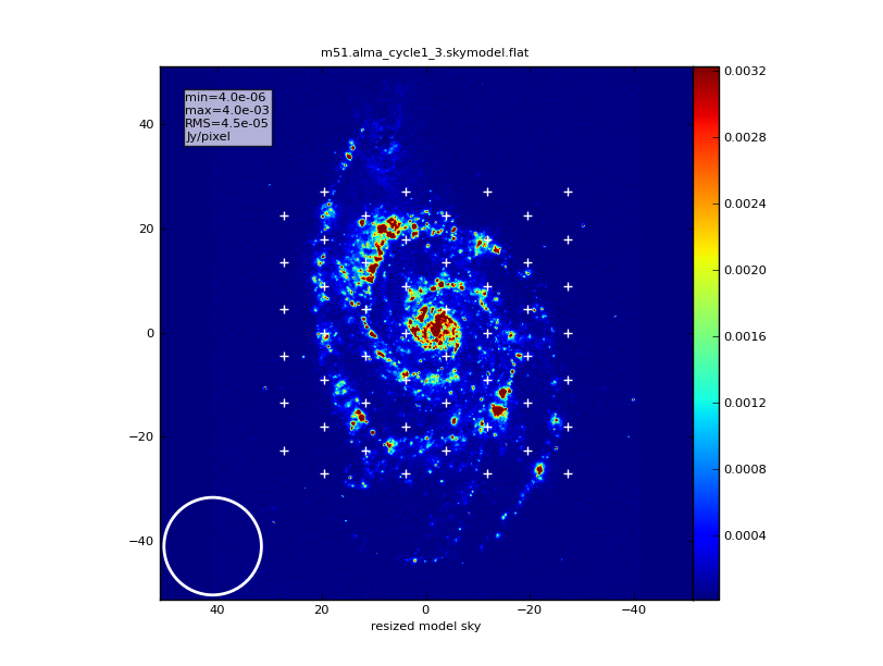
We will simulate observations using the main array in "configuration number 3" from Cycle 1. This configuration affords ~0.5 arcsec resolution.
antennalist="alma_cycle1_3.cfg"
We'll set the 12m array observing time to 2 hours:
totaltime="7800s"
Following the Cycle 1 convention, we will instruct simalma to observe 3 times longer with the 7m array and total power dishes.
acaratio=3.0
acaconfig="aca_cycle1.cfg"
We set the precipitable water vapor to 0.6 mm to represent observations in nominal weather. The simulation will add noise to the data based on this setting.
pwv=0.6
To cover all of the galaxy according to our rescaled pixel size, we'll need a 1 arcmin mosaic, and we'll let simalma calculate the pointings for us:
mapsize="1arcmin"
Finally you can check the input settings and run the simulation.
inp
go
What does it do?
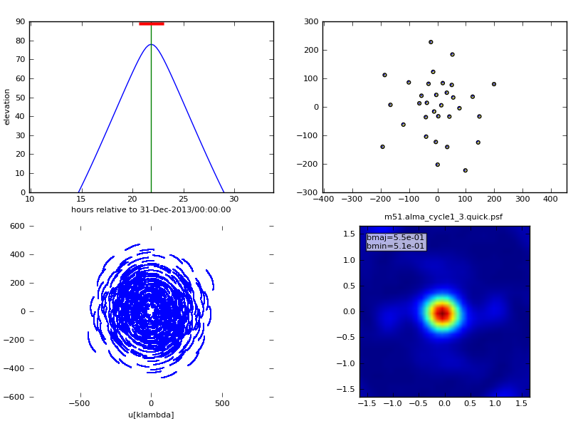
The 12m array observation is simulated first -- simalma simply calls simobserve with your input parameters. simobserve generates a graphic showing the elevation of the target and the synthesized dirty beam:
The 12m-only visibilities are not currently imaged separately from the 7m visibilities, but this is an expected upgrade in a future release. One could easily image the generated measurement set, which will be named according to the antennalist parameter above -- in this example, it is called m51.alma_cycle1_3.noisy.ms/.
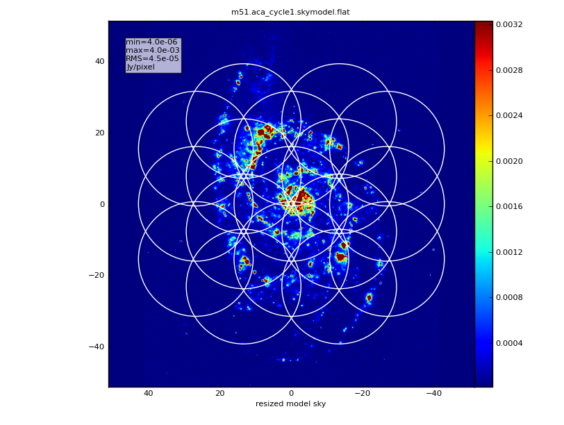
Next, the 7m ACA observation is simulated, with a second call to simobserve. simobserve follows the same conventions as the ALMA Observation Preparation Tool, and sets the mosaic pointings to cover the area requested. It takes fewer 7m pointings to cover the region than it did 12m pointings.
It is useful to know that a version of the input sky model convolved to the ACA resolution is generated, in this example m51.aca_cycle1.skymodel.flat.regrid.conv/. That image can be useful to better understand the simulation results.
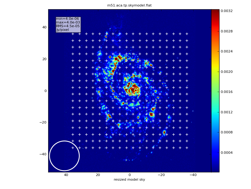
Next, simobserve is called a third time to generate the total power image. Again according to Cycle 1 conventions, the total power map covers the same region as the main array mosaic, except an extra pointing is added around the outside edge of the map so that the total power map is larger than the interferometric mosaic. (Total power maps usually have additional noise and artifacts at their edges). Furthermore, a square raster pattern is used instead of the hexagonal pattern of the interferometric array maps.
Deconvolve the visibilities back into images
Next simalma uses simanalyze to combine the three measurement sets and create a single image.
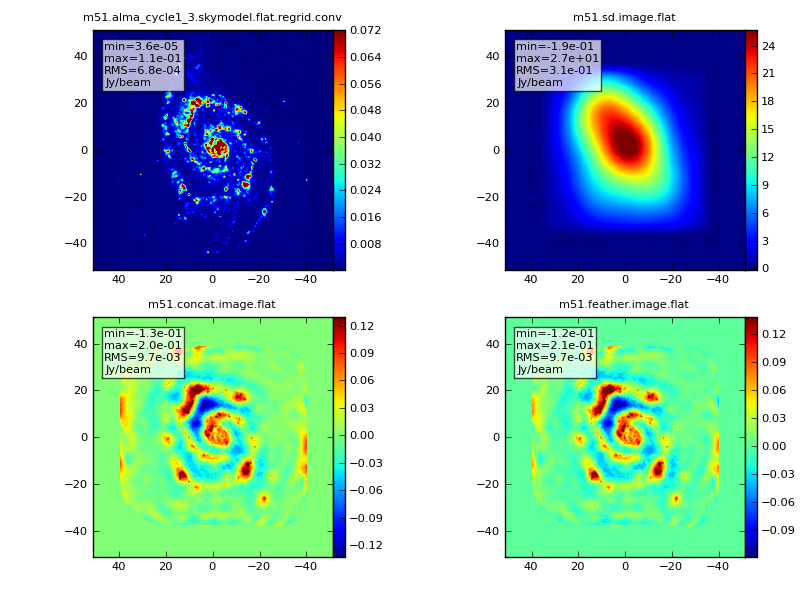
There are many ways to combine data from the separate observations. If you are dealing with real ALMA data, you may wish to discuss options with scientists at your ARC. Currently, simalma concatenates the two sets of interferometric visibilities first, images them, then separately images the total power observations, and finally uses the feather task to combine the two images.
The total power image is generated using gridding tools from the ASAP package inside of CASA. simalma attempts to find the optimal gridding kernel to achieve maximum sensitivity and resolution of the single dish map. (Finding optimal parameters is an area of active investigation.)
When combining interferometric data from different arrays "manually", it is critical to set the relative data weights properly. Simulated data have weights=1, since the thermal noise is generated uniformly per baseline. However, in reality the 7m baselines have lower sensitivity than the 12m baselines, and their weights must be decreased by the sensitivity ratio. simalma uses the visweightscale parameter of concat to apply that lower weight of (7/12)**2 to the 7m visibilities. If you wish to combine data manually, you must do this step yourself.
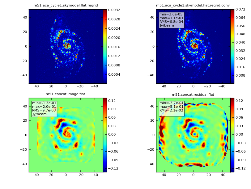
The concatenated visibilities are imaged, and diagnostic graphics with "concat" in their names are generated:
A note for those combining data by hand: When combining the single dish and interferometric maps in the image plane using the feather task, one must use the interferometric map <it>without</it> the primary beam correction, and first multiply the total power map by the interferometric sensitivity image (".flux") -- this ensures that noise effects are properly handled on the edges of each map, and do not grow artificially. After running feather, the output is masked to 0.2 times the interferometric primary beam, since the total power map was created larger than the interferometric map on purpose, so the edges of the combined image do not contain any interferometric information.:
Last checked on CASA Version 4.1.0.