PlanetPlots

Return to Analysis Utilities

This page documents the planetPlots function of Python module analysisUtils.

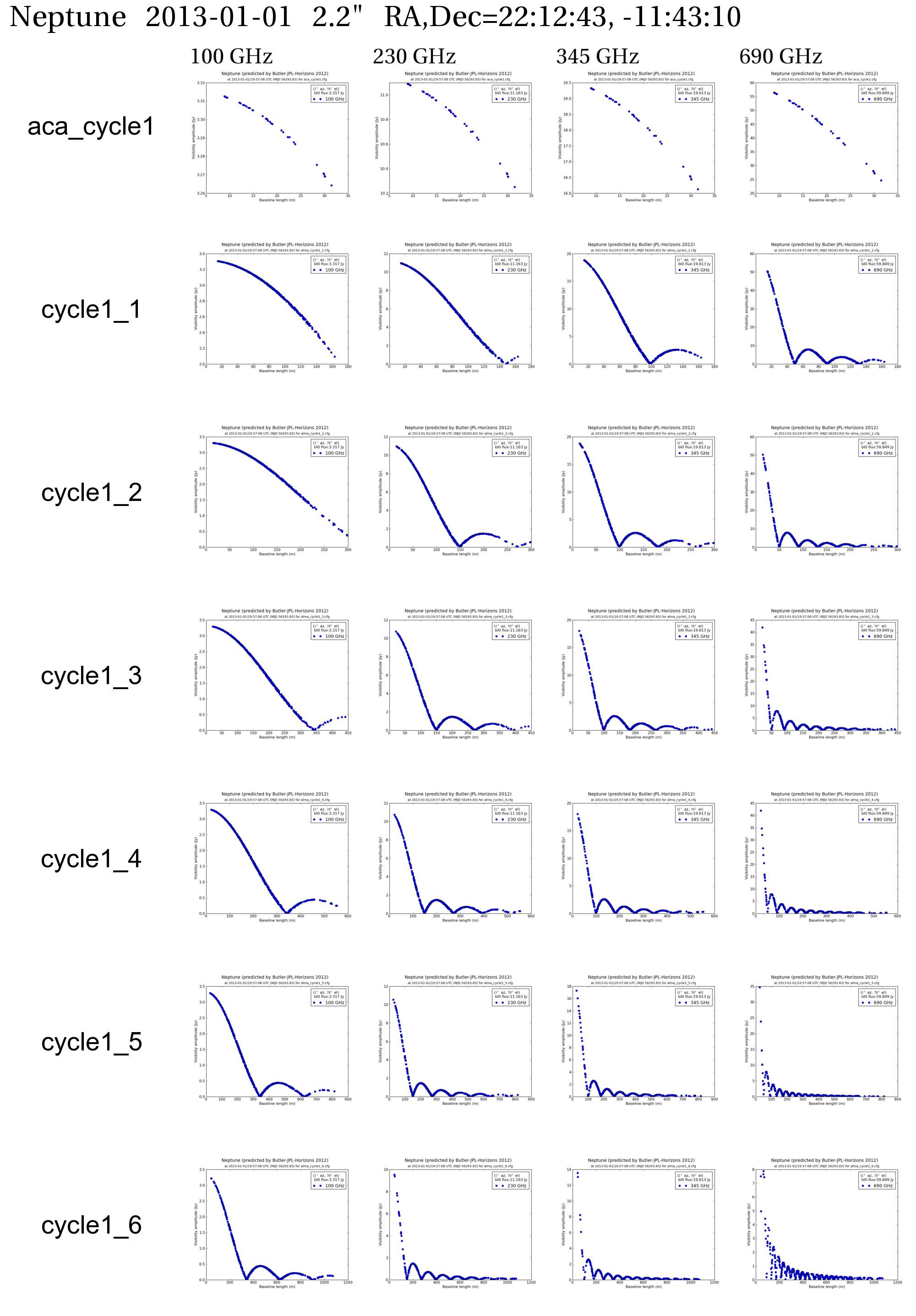
By calling predictcomp, this function will create uv amplitude vs. uvdistance visibility plots for a specified date for the specified objects, frequencies and ALMA configurations. The output is a multipage collection of a grid of plots, one page per object, where rows are configurations and columns are frequencies.

Usage

au.planetPlots(objects='Venus,Ceres,Vesta,Pallas,Juno,Jupiter,Callisto,Europa,Ganymede,Io,Titan,Uranus,Neptune', 
               date='2013-01-01', freqs = [100,230,345,690], pixels=800, standard = 'Butler-JPL-Horizons 2012', 
               alma_cycle=1, longitude=-67.7549, configs=None, showbl0flux=True, keepcl=False, keeppngs=False, 
               gs='gs, pdftk='pdftk')

objects: comma-delimited string of planetary bodies 
date: observing date, all plots are a 1-second snapshot at transit 
freqs: a list of frequencies, in GHz
pixels: the width of each individual image in pixels (the smallest fonts are easily readable at 800)
standard: the model in casa to use
longitude: the longitude of the observatory in degrees East of Greenwich (default = ALMA)
alma_cycle: 0 or 1 (will automatically fill in the configs offered)
configs: uses this if alma_cycle=None, specify a list of configurations, such as: ['alma_cycle1_1.cfg','alma_cycle1_2.cfg']
showbl0flux: True/False, list the zero-baseline flux density in the legend
keepcl: True/False, keep or remove the component lists generated by predictcomp
keeppngs: True/False, keep or remove the individual pngs (leaving only the PDFs)
gs: full path to ghostscript (in case it is not found in your path, but only used if pdftk is not found)
pdftk: full path to pdftk (in case it is not found in your path)

 Pre-defined lists of configurations:
    alma_cycle=0:  configs=['alma.cycle0.compact.cfg',
                            'alma.cycle0.extended.cfg',
                            '/net/yildun/export/data_1/thunter/alma/sim/configs/alma.cycle0.hybrid.cfg',
                            ]
    alma_cycle=1:  configs=['aca_cycle1.cfg','alma_cycle1_1.cfg',
                            'alma_cycle1_2.cfg','alma_cycle1_3.cfg',
                            'alma_cycle1_4.cfg','alma_cycle1_5.cfg',
                            'alma_cycle1_6.cfg']

See setjy for a list of bodies.

Examples

CASA <3>: au.planetPlots(date='2013-01-01')

complete PDF

Single page extracted for Neptune:

generated by casa-4.0.0