PlanetPlots: Difference between revisions
From CASA Guides
Jump to navigationJump to search
No edit summary |
|||
| Line 27: | Line 27: | ||
CASA <3>: au.planetPlots(date='2012-10-20') | CASA <3>: au.planetPlots(date='2012-10-20') | ||
</source> | </source> | ||
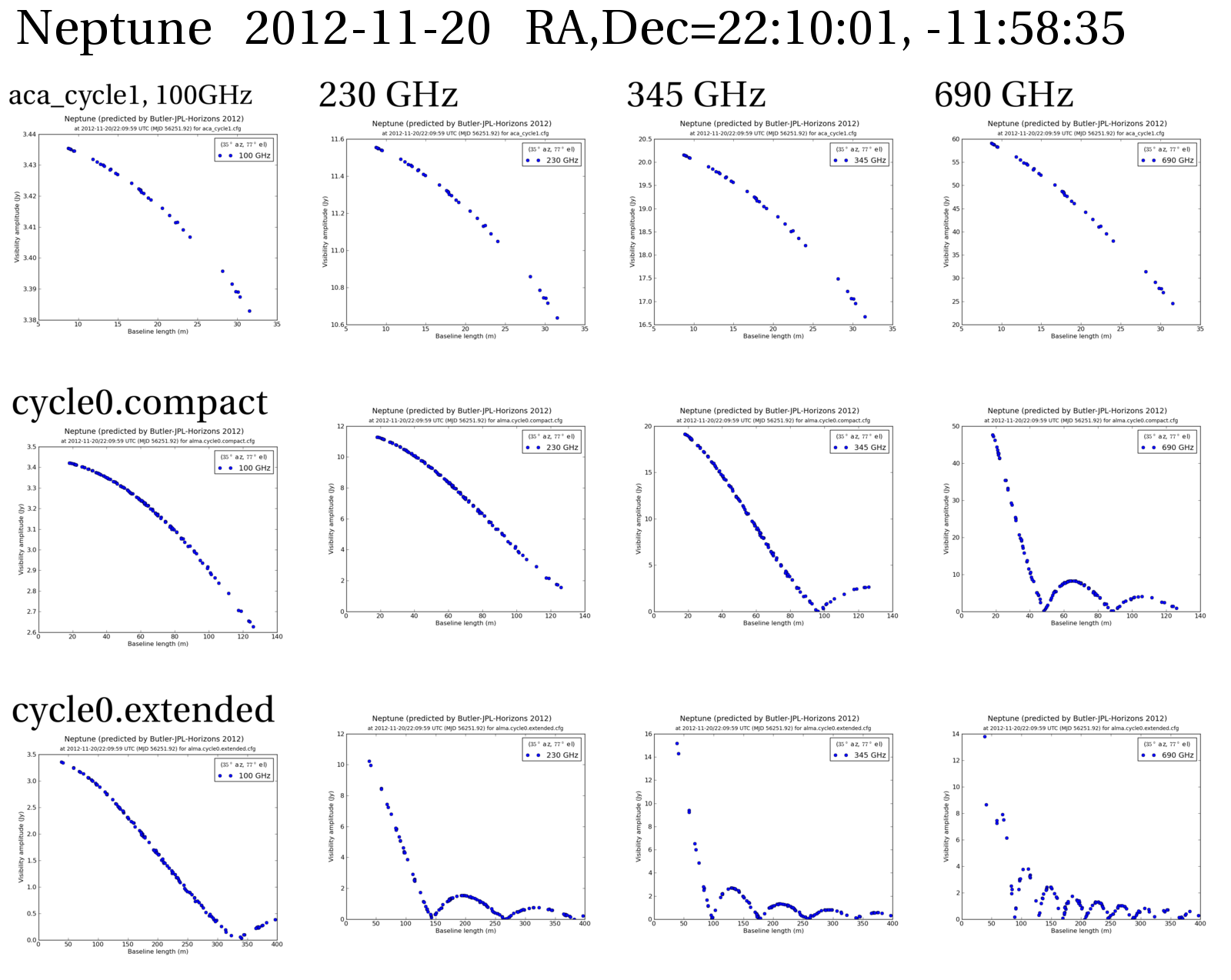
[[File:2012-11-20.pdf]] | |||
[[File:Neptune.2012-11-20.labeled.png|200px|thumb|left|alt text]] | |||
Revision as of 21:25, 8 October 2012
Return to Analysis Utilities
This page documents the planetPlots function of Python module analysisUtils.
This function will create uv amplitude vs. uvdistance visibility plots for the specified objects, date, frequencies and ALMA configurations. The output is a multipage collection of a grid of plots, one page per object, where rows are configurations and columns are frequencies.
Usage
au.planetPlots(objects='Venus,Ceres,Vesta,Pallas,Juno,Jupiter,Callisto,Europa,Ganymede,Io,Titan,Uranus,Neptune',
               date='2013-01-01', freqs = [100,230,345,690], standard = 'Butler-JPL-Horizons 2012',
               alma_cycle=1,configs=None)

objects: comma-delimited string of planetary bodies (see help setjy)
date: observing date, all plots are a 1-second snapshot at transit
freqs: a list of frequencies, in GHz
standard: the model in casa to use
alma_cycle: 0 or 1 (will automatically fill in the configs offered)
configs: alternative to alma_cycle, specify a list of configurations, such as: ['alma_cycle1_1.cfg','alma_cycle1_2.cfg']
Examples
CASA <3>: au.planetPlots(date='2012-10-20')
