MRK 6: red-shifted HI absorption 5.5.0: Difference between revisions
| Line 45: | Line 45: | ||
For the purposes of this tutorial, we are interested only in the source [http://en.wikipedia.org/wiki/B._E._Markarian Markarian] [http://nedwww.ipac.caltech.edu/cgi-bin/nph-objsearch?objname=mrk+6&extend=no&hconst=73&omegam=0.27&omegav=0.73&corr_z=1&out_csys=Equatorial&out_equinox=J2000.0&obj_sort=RA+or+Longitude&of=pre_text&zv_breaker=30000.0&list_limit=5&img_stamp=YES 6], but the reduction techniques could be applied to any of the sources in the measurement set. | For the purposes of this tutorial, we are interested only in the source [http://en.wikipedia.org/wiki/B._E._Markarian Markarian] [http://nedwww.ipac.caltech.edu/cgi-bin/nph-objsearch?objname=mrk+6&extend=no&hconst=73&omegam=0.27&omegav=0.73&corr_z=1&out_csys=Equatorial&out_equinox=J2000.0&obj_sort=RA+or+Longitude&of=pre_text&zv_breaker=30000.0&list_limit=5&img_stamp=YES 6], but the reduction techniques could be applied to any of the sources in the measurement set. | ||
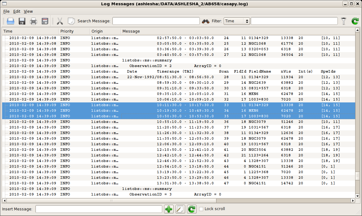
Using [[listobs]] and [[plotxy]] we learn the source names, spectral windows, and viable reference antennas. | [[File:MRK6-shot3.png|thumb|[[listobs|Listobs]] output for AB658. The data for MRK 6 and its calibrators are highlighted.]] | ||
Using [[listobs]] and [[plotxy]] we learn the source names, spectral windows, and viable reference antennas. A screenshot of the [[listobs]] output is given at right. | |||
{| border=1 | {| border=1 | ||
Revision as of 14:45, 9 February 2010
Overview
This example demonstrates a trickier spectral line data set. In this case, several radio bright active galaxies were observed to look for redshifted 21 cm absorption. The data were obtained using 4IF mode, which means that the full range of velocities were split into two spectral windows (in this example, CASA identifies them as spectral windows 14 and 15). Producing the data cube will require eventually stitching these windows back together. Happily, clean includes flexible regridding and interpolation in the spectral domain. Clean further allows you to adjust the velocity reference frame.
Retrieve the data from the NRAO archive
Download your data from the VLA Archive; in this example we'll use the publicly available survey AB658. These data were published in Gallimore et al. (1999).
With the present archive defaults, you should have obtained the following VLA archive files.
'AB658_A921122.xp1'
'AB658_A921122.xp2'
'AB658_A921122.xp3'
'AB658_A921122.xp4'
This tutorial broadly follows the techniques described in the continuum survey tutorial and the 21 cm emission tutorial, and the basic calibration steps are presented only in outline.
Loading the Data
Recall that the python file globber glob is your friend here!
measurementSet = "ab658.ms" # Store the desired name of the measurement set

from glob import glob
fileList = sorted(glob("AB658*.xp?"))

# double check to see if the file already exists
import os

if not os.path.isdir("./" + measurementSet): # measurement sets are directories
    importvla(archivefiles=fileList, vis=measurementSet) # only import if ab658.ms doesn't yet exist

vis = measurementSet
mode = "summary"
vishead
For the purposes of this tutorial, we are interested only in the source Markarian 6, but the reduction techniques could be applied to any of the sources in the measurement set.

Using listobs and plotxy we learn the source names, spectral windows, and viable reference antennas. A screenshot of the listobs output is given at right.
| Source | MKN6 |
| Amp Cal | 0134+329 = 3C48 |
| Phase Cal | 1003+830 |
| Central Antennas | VA27, VA09, VA23 |
| Spectral Window IDs | 14, 15 |
It's just as well to put that information into python global variables.
sourceName = "MKN6"
phaseCal = "1003+830"
ampCal = "0134+328"
refAnt = "VA27" # or perhaps "VA09" or "VA23"
spwStr = '14, 15'
The selection of the spectral windows, stored here in the string variable spwStr, is key to getting the calibration right. Each science target in the multisource measurement set has a tuning respective of the source redshift, and the calibration observations are matched to those spectral windows. Were the spectral windows parameter (usually spw) left to its default value (all available spectral windows), many calibration routines would necessarily fail.
Editing the Data

First inspect the data using plotms.
default(plotms)
vis = measurementSet
field = sourceName
plotms
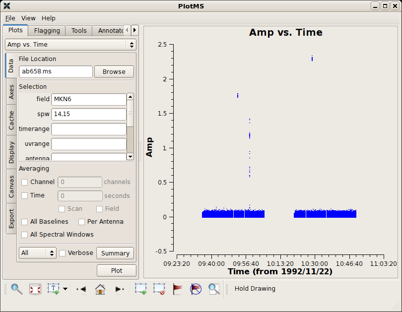
Be sure to select Axes → X Axis → Time and Axes → Y Axis → Amp (those settings are likely the default). There is some obvious junk isolated in time; see the screenshot at right. Follow the tutorial to flag discrepant data for the source and calibrators.
Calibration
Calibration of HI absorption spectra follows the basic techniques outlined in the continuum tutorial and HI emission tutorial.
First, set the flux of the amplitude calibrator. Notice that we are being careful to keep track of the spectral windows and not using the default spw.
# set the flux standard
default('setjy')
vis = measurementSet
field = ampCal
spw = spwStr # this is key to getting the calibration right!
casapath = os.environ.get('CASAPATH').split()[0]
modimage = ''
setjy()
Bandpass calibration comes next.
# bandpass calibration
default('bandpass')
vis = measurementSet
spw = spwStr # this is key to getting the calibration right!
caltable = btable
gaintable = ''
gainfield = ''
interp = ''
field = phaseCal
spw = ''
selectdata = False
gaincurve = False
opacity = 0.0
bandtype = 'B'
solint = 'inf'
combine = 'scan'
refant = refAnt
bandpass()

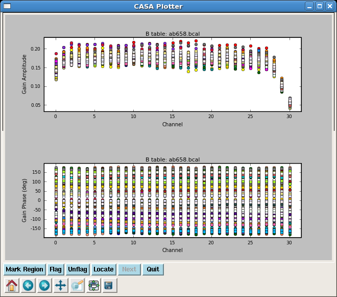
In order to perform the amplitude and phase calibrations, we'll need to inspect the bandpass response curve to select appropriate channels to average. We want to choose those channels where the response is relatively flat. The result of plotcal is shown at right: the bandpass is flat over channels 2:27.
# plot the bandpass calibration
default('plotcal')
spw = spwStr
caltable = btable
field = phaseCal
subplot = 211
yaxis = 'amp'
showgui = True
plotcal()
subplot = 212
yaxis = 'phase'
plotcal()
The following steps generate amplitude and phase solutions for the calibrators, and the fluxscale is bootstrapped from the amplitude calibrator onto the phase calibrator, effectively turning the phase calibrator into a local flux calibrator for the science target.
default('gaincal')
vis = measurementSet
caltable = gtable
gaintable = btable
gainfield = ''
interp = 'nearest'
field = ampCal + ',' + phaseCal
# specify data only from the flat region of the bandpass response
spw = '14:2~27,15:2~27'
selectdata = False
gaincurve = False
opacity = 0.0
gaintype = 'G'
solint = 'inf'
combine = ''
calmode = 'ap'
minsnr = 1.0
refant = refAnt
gaincal()
#=====================================================================
#
# Bootstrap flux scale
#
vis = measurementSet
# set the name for the output rescaled caltable
fluxtable = ftable
caltable = gtable
reference = ampCal
transfer = phaseCal
fluxscale()
The task fluxscale will give the bootstrapped flux density of the phase calibrator. If all goes well, something like the following should appear in the log window.
Beginning fluxscale--(MSSelection version)-------
 Found reference field(s): 0134+329
 Found transfer field(s):  1003+830
 Flux density for 1003+830 in SpW=14 is: 0.477297 +/- 0.000606617 (SNR = 786.818, nAnt= 26)
 Flux density for 1003+830 in SpW=15 is: 0.472778 +/- 0.000521238 (SNR = 907.03, nAnt= 26)
Storing result in ab658.fluxscale
We should inspect the calibration solutions to make sure they are reasonable, but we'll be cavalier and tread forward. Apply the calibrations to the science target and split that target into its own measurement set.
default('applycal')
vis = measurementSet
gaintable = [ftable,btable]
gainfield = [phaseCal,'*']
interp = ['linear','nearest']
field = sourceName
# choose the appropriate spectral windows
spw = spwStr
# by default, calibrations for a spectral window will map to the same
spwmap = []
selectdata = False
gaincurve = False
opacity = 0.0
applycal()
#
default('split')
vis = measurementSet
outputvis = splitms
field = sourceName
# weed out the end channels
spw = '14:2~27,15:2~27'
datacolumn = 'corrected'
split()
Continuum Subtraction
Ideally, we would use plotms to identify the channels where HI absorption is present (see the HI emission tutorial.) The absorption line is however isolated against the radio continuum and is not apparent in averaged visibilities. Instead, we'll have to produce a dirty cube using clean and inspect the spectrum in the image domain.