Antennae Band7 - Calibration for CASA 3.3: Difference between revisions
| (362 intermediate revisions by 6 users not shown) | |||
| Line 7: | Line 7: | ||
*'''This portion of the guide covers calibration of the raw visibility data. To skip to the imaging portion of the guide, see: [[Antennae Band7 - Imaging]]'''. | *'''This portion of the guide covers calibration of the raw visibility data. To skip to the imaging portion of the guide, see: [[Antennae Band7 - Imaging]]'''. | ||
== | ==Overview== | ||
This part of the Antennae Band 7 CASA guide will step you through the calibration of the visibility data. We will begin by flagging (marking as bad) data known to be useless before any inspection, for example data where one telescope blocks the line of sight of another. Then we will apply telescope-generated calibration tables to partially correct for atmospheric effects. After inspecting the data, we will flag some additional data that exhibit pathologies. Then we will use observations of the calibrators Titan and 3c279 to derive the phase and amplitude response of individual antennas as a function of time and frequency ("phase", "amplitude", and "bandpass" calibrations). We will apply these to the data and then extract the calibrated source data into a file appropriate for imaging. | |||
The general procedure in this guide follows the other ALMA CASA guides: [[NGC3256Band3]] and [[TWHydraBand7]]. | |||
==Unpack the Data== | |||
Once you have downloaded the Antennae_Band7_UnCalibratedMSandTablesForReduction.tgz, unpack the file in a terminal outside CASA using | Once you have downloaded the Antennae_Band7_UnCalibratedMSandTablesForReduction.tgz, unpack the file in a terminal outside CASA using | ||
> | <source lang="bash"> | ||
then change directory | tar -xvzf Antennae_Band7_UnCalibratedMSandTablesForReduction.tgz | ||
</source> | |||
then change directory to the new directory | |||
<source lang="bash"> | |||
cd Antennae_Band7_UnCalibratedMSandTablesForReduction | |||
</source> | |||
You may wish to type | You may wish to type | ||
>ls | <source lang="bash"> | ||
ls | |||
to look at the files present. You should see a | </source> | ||
to look at the files present. You should see a set of files with extension ".ms". These are CASA measurement set (MS) files. The data have already been converted to MS format from the native ALMA format using the CASA task {{importasdm}}. In addition to the data, we provide you with calibration tables containing system temperature (Tsys), water vapor radiometer (WVR), and antenna position information. For Early Science, these tables will either be pre-applied or supplied with the data. | |||
To begin, start CASA by typing | To begin, start CASA by typing | ||
>casapy | <source lang="bash"> | ||
casapy | |||
</source> | |||
Be sure that you are using the version indicated at the top of this page. | |||
==Initial Inspection== | ==Initial Inspection== | ||
First we will take stock of what we have. If you have not already done so, begin by reviewing the description of the observations here [[AntennaeBand7]] . The 10 data sets each target either the | First we will take stock of what we have. If you have not already done so, begin by reviewing the description of the observations here: [[AntennaeBand7]]. The 10 data sets each target either the Northern or the Southern Mosaic, as follows: | ||
Northern Mosaic: | Northern Mosaic: | ||
| Line 43: | Line 69: | ||
*uid___A002_X215db8_X392.ms | *uid___A002_X215db8_X392.ms | ||
The first step is to get basic information about the data: targets observed, time range, spectral setup, and so on. We do this using the task {{listobs}}, which will output a detailed summary of each dataset. | The first step is to get basic information about the data: targets observed, time range, spectral setup, and so on. We do this using the task {{listobs}}, which will output a detailed summary of each dataset. Enter the following commands into CASA: | ||
<source lang="python"> | <source lang="python"> | ||
| Line 54: | Line 80: | ||
"uid___A002_X215db8_X392"] | "uid___A002_X215db8_X392"] | ||
# Loop over each element in the list and | # Loop over each element in the list and create summary file using listobs | ||
for asdm in basename_all: | for asdm in basename_all: | ||
os.system('rm '+asdm+'.listobs.txt') | |||
listobs(vis=asdm+'.ms', listfile=asdm+'.listobs.txt', verbose=True) | |||
</source> | </source> | ||
Note that after cutting and pasting a 'for' loop like this you often have to press return twice to execute. You may also want to take care to paste a line at a time if you are having trouble copy and pasting. Even better, you can use "cpaste" to paste blocks of code. To do so type "cpaste" at the CASA prompt, paste your commands, and then type "--" and hit return on the final (otherwise empty) line. This should look something like this: | |||
<pre style="background-color: #fffacd;"> | |||
CASA <8>: cpaste | |||
Pasting code; enter '--' alone on the line to stop. | |||
:basename_all=["uid___A002_X1ff7b0_Xb","uid___A002_X207fe4_X3a","uid___A002_X207fe4_X3b9", | |||
: "uid___A002_X2181fb_X49","uid___A002_X1ff7b0_X1c8","uid___A002_X207fe4_X1f7", | |||
: "uid___A002_X207fe4_X4d7","uid___A002_X215db8_X18","uid___A002_X215db8_X1d5", | |||
: "uid___A002_X215db8_X392"] | |||
: | |||
:for asdm in basename_all: | |||
: print asdm | |||
:-- | |||
uid___A002_X1ff7b0_Xb | |||
uid___A002_X207fe4_X3a | |||
uid___A002_X207fe4_X3b9 | |||
uid___A002_X2181fb_X49 | |||
uid___A002_X1ff7b0_X1c8 | |||
uid___A002_X207fe4_X1f7 | |||
uid___A002_X207fe4_X4d7 | |||
uid___A002_X215db8_X18 | |||
uid___A002_X215db8_X1d5 | |||
uid___A002_X215db8_X392 | |||
CASA <9>: | |||
</pre> | |||
cpaste should be ''much'' more robust than copying-and-pasting directly into the shell but if you have trouble, just carefully paste one line at a time directly into CASA and hit return until the desired command executes. | |||
You can browse through the listobs output as you would normally look at a text file (use emacs, vi, or another editor). You can also send the output to the terminal from inside of CASA. To do so type: | These commands define a python list called "basename_all", which contains the name of all 10 MS files. The "for" loop executes for each element in basename_all, calling listobs and directing the output to a file called, e.g., "uid___A002_X1ff7b0_Xb.listobs.txt" for the first measurement set. You can browse through the listobs output as you would normally look at a text file (use emacs, vi, or another editor). You can also send the output to the terminal from inside of CASA. To do so type: | ||
<source lang="python"> | <source lang="python"> | ||
| Line 77: | Line 133: | ||
CASA knows a few basic shell commands like 'cat', 'ls', and 'rm' but for more complex commands you will need to run them inside 'os.system("command")'. For more information see http://casa.nrao.edu/ . | CASA knows a few basic shell commands like 'cat', 'ls', and 'rm' but for more complex commands you will need to run them inside 'os.system("command")'. For more information see http://casa.nrao.edu/ . | ||
Here is an example of the (abridged) output from {{listobs}} for the first dataset in the list, uid___A002_X1ff7b0_Xb.ms, which targets the Northern Mosaic: | Here is an example of the (abridged) output from {{listobs}} for the first dataset in the list, uid___A002_X1ff7b0_Xb.ms, which targets the Northern Mosaic. You would see this if you had specified '''verbose''' to be False in the listobs call: | ||
<pre style="background-color: #fffacd;"> | <pre style="background-color: #fffacd;"> | ||
| Line 136: | Line 192: | ||
</pre> | </pre> | ||
And here is an | And here is an extract from the full '''verbose''' {{listobs}} for uid___A002_X1ff7b0_X1c8.ms, which targets the Southern Mosaic (note that we have snipped out the record of individual scans): | ||
<pre style="background-color: #fffacd;"> | <pre style="background-color: #fffacd;"> | ||
================================================================================ | |||
MeasurementSet Name: /export/lustre/aleroy/Antennae_Band7_UnCalibratedMSandTablesForReduction/uid___A002_X1ff7b0_X1c8.ms MS Version 2 | |||
================================================================================ | |||
Observer: Unknown Project: T.B.D. | |||
Observation: ALMA | |||
Data records: 175615 Total integration time = 4927.1 seconds | |||
Observed from 28-May-2011/02:50:18.2 to 28-May-2011/04:12:25.3 (UTC) | |||
<snip> | |||
Fields: 33 | |||
ID Code Name RA Decl Epoch SrcId nVis | |||
0 none 3c279 12:56:11.16657 -05.47.21.5247 J2000 0 12232 | |||
1 none Titan 12:42:44.82765 -01.43.41.4224 J2000 1 10615 | |||
2 none 3c279 12:56:11.16600 -05.47.21.5250 J2000 2 27764 | |||
3 none Antennae 12:01:53.17008 -18.52.37.9200 J2000 3 4829 | |||
4 none Antennae 12:01:52.18699 -18.53.30.3952 J2000 3 3883 | |||
5 none Antennae 12:01:52.64413 -18.53.26.6494 J2000 3 3883 | |||
6 none Antennae 12:01:53.10127 -18.53.22.9035 J2000 3 3872 | |||
7 none Antennae 12:01:53.55841 -18.53.19.1577 J2000 3 4818 | |||
8 none Antennae 12:01:54.01554 -18.53.15.4119 J2000 3 4829 | |||
9 none Antennae 12:01:54.47268 -18.53.11.6661 J2000 3 4829 | |||
10 none Antennae 12:01:54.92982 -18.53.07.9203 J2000 3 3872 | |||
11 none Antennae 12:01:55.38696 -18.53.04.1744 J2000 3 3883 | |||
12 none Antennae 12:01:55.84409 -18.53.00.4286 J2000 3 4840 | |||
13 none Antennae 12:01:56.30123 -18.52.56.6828 J2000 3 4818 | |||
14 none Antennae 12:01:52.18700 -18.53.22.9033 J2000 3 4829 | |||
15 none Antennae 12:01:52.64414 -18.53.19.1575 J2000 3 4818 | |||
16 none Antennae 12:01:53.10128 -18.53.15.4116 J2000 3 4818 | |||
17 none Antennae 12:01:53.55842 -18.53.11.6658 J2000 3 4840 | |||
18 none Antennae 12:01:54.01555 -18.53.07.9200 J2000 3 3872 | |||
19 none Antennae 12:01:54.47269 -18.53.04.1742 J2000 3 4829 | |||
20 none Antennae 12:01:54.92983 -18.53.00.4284 J2000 3 4829 | |||
21 none Antennae 12:01:55.38697 -18.52.56.6825 J2000 3 4829 | |||
22 none Antennae 12:01:55.84410 -18.52.52.9367 J2000 3 4829 | |||
23 none Antennae 12:01:51.72988 -18.53.19.1572 J2000 3 4818 | |||
24 none Antennae 12:01:52.18702 -18.53.15.4114 J2000 3 4829 | |||
25 none Antennae 12:01:52.64415 -18.53.11.6656 J2000 3 4829 | |||
26 none Antennae 12:01:53.10129 -18.53.07.9197 J2000 3 2266 | |||
27 none Antennae 12:01:53.55843 -18.53.04.1739 J2000 3 2266 | |||
28 none Antennae 12:01:54.01557 -18.53.00.4281 J2000 3 3212 | |||
29 none Antennae 12:01:54.47270 -18.52.56.6823 J2000 3 3234 | |||
30 none Antennae 12:01:54.92984 -18.52.52.9365 J2000 3 3212 | |||
31 none Antennae 12:01:55.38698 -18.52.49.1906 J2000 3 2266 | |||
32 none Antennae 12:01:55.84411 -18.52.45.4448 J2000 3 3223 | |||
(nVis = Total number of time/baseline visibilities per field) | |||
Spectral Windows: (9 unique spectral windows and 2 unique polarization setups) | |||
SpwID #Chans Frame Ch1(MHz) ChanWid(kHz) TotBW(kHz) Corrs | |||
0 4 TOPO 184550 1500000 7500000 I | |||
1 3840 TOPO 344845.586 488.28125 1875000 XX YY | |||
2 1 TOPO 343908.086 1875000 1875000 XX YY | |||
3 3840 TOPO 356845.586 488.28125 1875000 XX YY | |||
4 1 TOPO 343908.086 1875000 1875000 XX YY | |||
5 128 TOPO 344900.518 15625 2000000 XX YY | |||
6 1 TOPO 343892.705 1796875 1796875 XX YY | |||
7 128 TOPO 356900.518 15625 2000000 XX YY | |||
8 1 TOPO 343892.705 1796875 1796875 XX YY | |||
Antennas: 11: | |||
ID Name Station Diam. Long. Lat. | |||
0 DV02 A015 12.0 m -067.45.15.3 -22.53.26.0 | |||
1 DV04 J505 12.0 m -067.45.18.0 -22.53.22.8 | |||
2 DV06 T704 12.0 m -067.45.16.2 -22.53.22.1 | |||
3 DV07 A004 12.0 m -067.45.15.9 -22.53.28.0 | |||
4 DV08 A072 12.0 m -067.45.12.6 -22.53.24.0 | |||
5 DV09 A008 12.0 m -067.45.15.4 -22.53.26.8 | |||
6 DV10 A009 12.0 m -067.45.16.1 -22.53.26.1 | |||
7 DV11 A016 12.0 m -067.45.16.4 -22.53.25.1 | |||
8 PM01 T702 12.0 m -067.45.18.6 -22.53.24.1 | |||
9 PM02 A017 12.0 m -067.45.15.9 -22.53.26.8 | |||
10 PM03 J504 12.0 m -067.45.17.0 -22.53.23.0 | |||
</pre> | </pre> | ||
This output shows that three sources were observed in each data set: 3c279, Titan, and the Antennae. | This output shows that three sources were observed in each data set: 3c279, Titan, and the Antennae. | ||
* The '''Antennae''' are our science target. Note that the source name changes between the Northern and Southern Mosaic | * The '''Antennae''' are our science target. Note that the source name changes between the Northern Mosaic, where it is "NGC4038 - Antennae", and the Southern Mosaic, where it is just "Antennae". Also note that the source corresponds to a number of individual fields (see the Field ID column). These are the individual mosaic pointings. There are 23 for the Northern Mosaic and 29 for the Southern Mosaic. | ||
* '''Titan''' will be used to set the absolute flux scale of the data. | * '''Titan''' is observed once and will be used to set the absolute flux scale of the data. | ||
* '''3c279''' plays two roles: it will serve as our bandpass calibrator, | * '''3c279''' plays two roles: it will serve as our bandpass calibrator, to characterize the frequency response of the antennas, and because it is fairly close on the sky to the Antennae (18.6 degrees away) it will serve as our secondary calibrator (also referred to as the "phase calibrator" or "gain calibrator"), to track changes in the phase and amplitude response of the telescopes over time. Observations of 3c279 are interleaved with observations of the Antennae. | ||
The output also shows that the data contain many spectral windows | The output also shows that the data contain many spectral windows. Using the labeling scheme in the listobs above these are: | ||
* '''spw 0''' targets ~185 GHz and holds water vapor radiometer data | * '''spw 0''' targets ~185 GHz and holds water vapor radiometer data | ||
* '''spw 1''' and '''spw 3''' hold our science data. These are "Frequency Domain Mode" (FDM) data with small (0.49 | * '''spw 1''' and '''spw 3''' hold our science data. These are "Frequency Domain Mode" (FDM) data with small (0.49 MHz) channel width and wide (1.875 GHz) total bandwidth. As a result these have a lot of channels (3840). spw 1 holds the lower sideband (LSB) data and includes the CO(3-2) line. We will focus on these data. For the CO(3-2) line the channel width corresponds to 0.426 km/s and the bandwidth of spw 1 to 1634 km/s. | ||
* '''spw 2''' and '''spw 4''' hold frequency-averaged versions of spw 1 and 3 ("Channel 0" for those familiar with AIPS). These are used for quick inspection. We will not use them here. | * '''spw 2''' and '''spw 4''' hold frequency-averaged versions of spw 1 and 3 ("Channel 0" for those familiar with AIPS). These are used for some quick automated inspection. We will not use them here but we will carry out an equivalent inspection using spw 1. | ||
* '''spw 5''' and '''spw 7''' hold lower resolution processing ("Time Domain Mode", TDM) data | * '''spw 5''' and '''spw 7''' hold lower a resolution processing ("Time Domain Mode", TDM) of the data from the same part of the spectrum (baseband) as spws 1 and 3. These data have only 128 channels across 2 GHz bandwidth and so have a much coarser channel spacing than the FDM data. These were used to generate the calibration tables that we include in the tarball but will not otherwise appear in this guide. | ||
The final column of the listobs output in the logger (not shown above) gives the scan intent. Later we will use this information to flag the pointing scans and the hot and ambient load calibration scans. | The final column of the listobs output in the logger (not shown above) gives the scan intent. Later we will use this information to flag the pointing scans and the hot and ambient load calibration scans. | ||
| Line 161: | Line 285: | ||
We'll now have a look at the configuration of the antennas used to take the data using the task {{plotants}} (Figure 1). | We'll now have a look at the configuration of the antennas used to take the data using the task {{plotants}} (Figure 1). | ||
[[File:Uid_A002_X1ff7b0_Xb.ANT.png|200px|thumb|right|Fig. 1. Position of antennas in dataset uid_A002_X1ff7b0_Xb obtained using task {{plotants}}]] | [[File:Uid_A002_X1ff7b0_Xb.ANT.png|200px|thumb|right|'''Fig. 1.''' Position of antennas in dataset uid_A002_X1ff7b0_Xb obtained using task {{plotants}}]] | ||
<source lang="python"> | <source lang="python"> | ||
# In CASA | # In CASA | ||
| Line 175: | Line 299: | ||
</source> | </source> | ||
This will loop through all 10 data sets, show you the antenna position for each, and save that as a file named, e.g., "uid___A002_X1ff7b0_Xb.plotants.png" for the first data set. The "raw_input" command asks CASA to wait for your input before proceeding. | This will loop through all 10 data sets, show you the antenna position for each, and save that as a file named, e.g., "uid___A002_X1ff7b0_Xb.plotants.png" for the first data set. The "raw_input" command asks CASA to wait for your input before proceeding. If you would prefer to just browse the .png files after the fact you can remove this. Notice that the antenna setup changes, but only slightly, over the course of the 10 data sets. | ||
==How to Deal With 10 Measurement Sets== | ==How to Deal With 10 Measurement Sets== | ||
| Line 196: | Line 320: | ||
</source> | </source> | ||
You only need to define your list of MS files once per CASA session. Then "basename_all" will be a variable in the casapy shell. You can check if it exists by typing "print basename_all". In the interests of allowing you to easily exit and restart CASA and pick this guide up at any point we will redefine "basename_all" in each section of the guide. Feel free to skip this step if you've already defined it in your session. | |||
This page will step you through the reduction of the whole Antennae Band 7 SV data set using these 'for' loops. We will not be able to show every diagnostic plot but we give an example of each and the syntax to generate the rest. Also please be aware that even on a very fast machine this whole process can take a while, we are simply dealing with a lot of data. | |||
One potential "gotcha" is that the source name changes between the two data sets. Therefore at several points we will break apart our loop to iterate separately over the Northern and Southern Mosaics, where the source can be referred unambiguously. Another subtle point is that 3c279 appears with two distinct field IDs in the Southern Mosaic, but only one in the Northern Mosaic. We will largely avoid this by referring to the source by its name but if you tried to use field ID numbers and mingled the two data sets this could cause confusion. | |||
==''A Priori'' Flagging== | |||
Even before we look in detail, we know that there are some data that we wish to exclude. We will start by flagging "shadowed" data where one antenna blocks the line of sight of another. We will also flag scans that were used to carry out pointing and atmospheric calibration, identified by their scan intent. Finally, we'll flag the autocorrelation data (the correlation of the signal from an antenna with itself) as we are only interested in cross-correlation data to make an interferometric image. | |||
Start by defining our list of MS files: | |||
<source lang="python"> | |||
# In CASA | |||
basename_all=["uid___A002_X1ff7b0_Xb","uid___A002_X207fe4_X3a","uid___A002_X207fe4_X3b9", | |||
"uid___A002_X2181fb_X49","uid___A002_X1ff7b0_X1c8","uid___A002_X207fe4_X1f7", | |||
"uid___A002_X207fe4_X4d7","uid___A002_X215db8_X18","uid___A002_X215db8_X1d5", | |||
"uid___A002_X215db8_X392"] | |||
</source> | |||
You may want to reset the flagging if you have tried this step before and are starting over though this is not necessary on your first time through. Do so using {{flagdata}}: | |||
<source lang="python"> | |||
# In CASA | |||
for asdm in basename_all: | |||
print "Reseting flags for "+asdm | |||
flagdata(vis=asdm+'.ms',mode='manualflag', unflag=T, flagbackup=F) | |||
</source> | |||
Then flag shadowed data using the command {{flagdata}}: | |||
<source lang="python"> | |||
# In CASA | |||
for asdm in basename_all: | |||
print "Flagging shadowed data for "+asdm | |||
flagdata(vis=asdm+'.ms',mode = 'shadow', diameter=12.0, flagbackup = F) | |||
</source> | |||
In the {{flagdata}} task we choose: | |||
* '''vis''' = asdm+'.ms' : each measurement set | |||
* '''mode''' = 'shadow',diameter=12.0: flag shadowed data, taking into account that antennas are 12m diameter | |||
* '''flagbackup''' = F: Do not automatically back up the flag files. We will save all of the ''a priori'' flags together using {{flagmanager}} at the end of this subsection and save some space and time. | |||
: | |||
: | |||
The relevant calibration information has already been extracted from the pointing and atmospheric scans and we will not need them below. Now flag the pointing scans using {{flagdata}} in 'manualflag' mode and selecting on 'intent': | |||
</ | <source lang="python"> | ||
# In CASA | |||
for asdm in basename_all: | |||
print "Flagging calibration scans for "+asdm | |||
flagdata(vis=asdm+'.ms', mode='manualflag', intent='*POINTING*', flagbackup = F) | |||
</source> | |||
Note that because the atmospheric calibration scans contain only TDM spectral windows, they will be removed automatically when we separate out the FDM data below. | |||
Now flag the autocorrelation data: | |||
<source lang="python"> | |||
# In CASA | |||
for asdm in basename_all: | |||
print "Flagging autocorrelation data for "+asdm | |||
flagdata(vis=asdm+'.ms',autocorr=True,flagbackup=F) | |||
</source> | |||
Finally store the current flags information using {{flagmanager}}: | |||
== | <source lang="python"> | ||
# In CASA | |||
for asdm in basename_all: | |||
print "Backing up 'a priori' flags for "+asdm | |||
flagmanager(vis = asdm+'.ms', mode = 'save', versionname = 'Apriori') | |||
</source> | |||
Where '''versionname''' is just the name we assign to the current flagging state in the data. We can now roll back the flags to match the current version, called 'Apriori', whenever we want. There is no reason to do this now, but the syntax would be: | |||
<source lang="python"> | <source lang="python"> | ||
# In CASA | # In CASA | ||
for asdm in basename_all: | |||
print "Resorting up 'a priori' flags for "+asdm | |||
flagmanager(vis = asdm+'.ms', mode = 'restore', versionname = 'Apriori') | |||
</source> | |||
It would have been possible to set {{flagdata}} to '''flagbackup'''=T so that it stores the flags at each of the flagging step automatically, but this way it is a bit more efficient with regard to time and disk space. More important, lumping all the ''a priori'' flagging together gives us a natural point to roll back to if we get in trouble. | |||
<pre style="background-color: #E0FFFF;"> | |||
The flagmanager task will also allow you to view the saved flagging versions, | |||
including those created by running flagdata with flagbackup=T. | |||
For example try | |||
flagmanager(vis='uid___A002_X2181fb_X49.ms', mode='list') | |||
The output in the logger should list the Apriori flagging that we have applied. | |||
It will also indicate versions associated with any flagdata command where you | |||
did not set flagbackup=F. Other tasks, for example applycal, will also create | |||
flag version tables. | |||
</pre> | |||
==Examine and Apply Tsys, WVR, and Antenna Position Calibration Tables Then Split== | |||
The Antennae_Band7_UnCalibratedMSandTablesForReduction directory includes system temperature (Tsys), water vapor radiometer (WVR), and antenna position calibration tables, which appear as files with extensions '.tsys.cal.fdm', '.wvr.cal', and '.antpos'. The WVR and Tsys tables have been built from the spw 0 (WVR) and spw 5 & 7 (Tsys) data. We provide these to you because CASA does not generate them at the moment, a situation that will change soon. The Tsys calibration gives a first-order correction for the atmospheric opacity as a function of time and frequency and associates weights with each visibility that persists through imaging. The WVR calibration uses observations of the wings of the 183 GHz atmospheric water line to correct for phase variations as a function of time. The antenna position table reflects refinements in the measured positions of the antennas from those stored in the data. | |||
We inspect the Tsys tables for the spectral window spw=1 with the task {{plotcal}}. We want to check that Tsys data have reasonable values and identify any unexpected features as a function of either time or frequency. To get an idea of sensible Tsys under average atmospheric observations consult the ALMA sensitivity calculator, accessible from http://www.almascience.org . | |||
We start by plotting the Tsys for all the antennas and polarizations (XX and YY) as a function of time for each. Here and throughout we focus on spw 1, which contains CO(3-2): | |||
[[File:uid___A002_X1ff7b0_X1c8.tsys_vs_time.page1.png|200px|thumb|right|'''Fig. 2a.''' Tsys vs. time plot for uid_A002_X1ff7b0_Xb (northern mosaic). First 8 antennas. Note the high y-axis values for DV04. The two different colors indicate the two polarizations (XX and YY).]] | |||
[[File:uid___A002_X1ff7b0_X1c8.tsys_vs_time.page2.png|200px|thumb|right|'''Fig. 2b.''' Tsys vs. time plot for uid_A002_X1ff7b0_Xb (northern mosaic). Remaining antennas.]] | |||
<source lang="python"> | |||
#In CASA | |||
basename_all=["uid___A002_X1ff7b0_Xb","uid___A002_X207fe4_X3a","uid___A002_X207fe4_X3b9", | basename_all=["uid___A002_X1ff7b0_Xb","uid___A002_X207fe4_X3a","uid___A002_X207fe4_X3b9", | ||
"uid___A002_X2181fb_X49","uid___A002_X1ff7b0_X1c8","uid___A002_X207fe4_X1f7", | "uid___A002_X2181fb_X49","uid___A002_X1ff7b0_X1c8","uid___A002_X207fe4_X1f7", | ||
"uid___A002_X207fe4_X4d7","uid___A002_X215db8_X18","uid___A002_X215db8_X1d5", | "uid___A002_X207fe4_X4d7","uid___A002_X215db8_X18","uid___A002_X215db8_X1d5", | ||
"uid___A002_X215db8_X392"] | "uid___A002_X215db8_X392"] | ||
for asdm in basename_all: | |||
print "Plotting Tsys vs. time for "+asdm | |||
plotcal(caltable=asdm+'.tsys.cal.fdm', | |||
xaxis="time",yaxis="amp", | |||
spw='1:1200~1200',plotsymbol=".", subplot=421, | |||
antenna='0~7', | |||
iteration='antenna', figfile=asdm+'.tsys_vs_time.page1.png', | |||
fontsize=6.0) | |||
#dummy_string = raw_input("First eight antennas for "+asdm+" . Hit <Enter> to continue.") | |||
plotcal(caltable=asdm+'.tsys.cal.fdm', | |||
xaxis="time",yaxis="amp", | |||
antenna='8~15', | |||
spw='1:1200~1200',plotsymbol=".", subplot=421, | |||
iteration='antenna', figfile=asdm+'.tsys_vs_time.page2.png', | |||
fontsize=6.0) | |||
#dummy_string = raw_input("Remaining antennas for "+asdm+" . Hit <Enter> to continue.") | |||
</source> | </source> | ||
Now we | This sequence loops over all of our files and plots Tsys as a function of time for channel 1200 in spectral window 1. In the call to {{plotcal}}: | ||
* '''subplot'''=421 parameter sets up a 4 x 2 panel grid. | |||
* '''iteration''' tells {{plotcal}} to make a separate plot for each antenna. | |||
* '''spw''' '1:1200~1200' selects spw '1' channel 1200-1200. This allows us to cleanly separate time variations from frequency variations. | |||
Because 8 panels is not enough to show all antennas on one page, there are two plotcal calls: one for the first 8 antennas ('''antenna'''=0~7) and one for any remaining antennas ('''antenna'''=8~15). The '''fontsize''' needs to be set to a small value or the text overlaps. | |||
The 'raw_input' commands will wait for you to hit Enter before issuing the next plot command. In the example above these are commented out (the leading "#" means that CASA will ignore them). If you would like to interactively cycle through the plots, uncomment them by removing the "#". Otherwise, the '''figfile''' parameter directs the output to .png files for later inspection. The easiest way to look at the 20 plots produced here is to simply inspect the .png files using your favorite viewer. | |||
The Tsys values in Figure 2 look reliable, with typical values ~150 K except for some large values of Tsys at ~300 and 400 K for DV04. We will flag the data for that antenna later. | |||
We will also want to look at Tsys as a function of frequency. The following commands step through how you would do this, but ''do not execute this command blindly!'' (just in case, we have included a "break" that you will need to remove before running or the "for" loop will simply cancel). The commands are similar to the Tsys vs. time {{plotcal}} but will take ''much'' longer to run because instead of tracking a single channel we now plot the data for all 3840 channels in spw 1. Future enhancements to CASA will make it possible to plot these data more efficiently (e.g., by stepping across channels) but for now it takes a long time to generate these plots. We have included them in the directory "tsys_plots/" in the distribution you downloaded so that you will not need to generate them yourself. If you ''really'' want to run this command, remove the "break" and run the commands: | |||
<source lang="python"> | |||
#In CASA | |||
for asdm in basename_all: | |||
break | |||
print "Plotting Tsys vs. frequency for "+asdm | |||
plotcal(caltable=asdm+'.tsys.cal.fdm', | |||
xaxis="freq",yaxis="amp", | |||
spw='1', plotsymbol=".", subplot=421, | |||
iteration='antenna', figfile=asdm+'.tsys_vs_freq.page1.png', | |||
antenna='0~7', fontsize=6.0) | |||
#dummy_string = raw_input("Inspecting Tsys table for "+asdm+" . Hit <Enter> to continue.") | |||
plotcal(caltable=asdm+'.tsys.cal.fdm', | |||
xaxis="freq",yaxis="amp", | |||
spw='1', plotsymbol=".", subplot=421, | |||
iteration='antenna', figfile=asdm+'.tsys_vs_freq.page2.png', | |||
antenna='8~15', fontsize=6.0) | |||
#dummy_string = raw_input("Inspecting Tsys table for "+asdm+" . Hit <Enter> to continue.") | |||
</source> | |||
[[File:uid___A002_X1ff7b0_X1c8.tsys_vs_freq.page1.png|200px|thumb|right|'''Fig. 3a.''' Tsys vs. frequency plot for uid_A002_X1ff7b0_Xb (northern mosaic). First 8 antennas. Note the high y-axis values for DV04 and the telluric ozone line near 343.2 GHz.]] | |||
[[File:uid___A002_X1ff7b0_X1c8.tsys_vs_freq.page2.png|200px|thumb|right|'''Fig. 3b.''' Tsys vs. frequency plot for uid_A002_X1ff7b0_Xb (northern mosaic). Remaining antennas.]] | |||
[[File:uid___A002_X215db8_X392.tsys_vs_freq.page2.png|200px|thumb|right|'''Fig. 3c.''' Tsys vs. frequency plot for uid___A002_X215db8_X392. Note the pathological behavior for DV12.]] | |||
Now have a look at the Tsys vs. frequency plots or see Figure 3 for an example on the first data set. You can see the effect of a close pair of atmospheric ozone absorption lines at about 343.2 GHz that makes Tsys larger near that frequency in all antennas. Applying the Tsys calibration tables will minimize the contribution of these atmospheric lines. Again DV04 stands out with its very high Tsys. Although not present in the first data sets, Antenna DV12 exhibits periodic spikes in Tsys vs. frequency for one polarization (see Figure 3c for an example from a later data set). It may or may not be possible to calibrate that behavior out. We will make a note to look carefully at DV12 further on in the calibration process. | |||
We are now ready to apply the Tsys and the WVR calibration tables to the data with {{applycal}}, which reads the specified gain calibration tables, applies them to the (raw) data column, and writes the calibrated results into the corrected column. Again, we loop through all the datasets. It is important to only apply Tsys and WVR corrections obtained close in time to the data being corrected, so in addition to looping over data sets we define the list of unique source names and loop over these. Then by setting '''gainfield''' and '''field''' to the same value we ensure that Tsys and WVR calibrations are only applied to the source for which they are measured. Because the source has a different name in the Northern Mosaic and the Southern Mosaic, we will carry out two loops. We will only correct '''spw''' 1, our science window, because we will drop the other data in a moment. | |||
<source lang="python"> | <source lang="python"> | ||
# In CASA | # In CASA | ||
for asdm in | |||
# A new list of file names that contain only data from the Northern Mosaic | |||
basename_north=["uid___A002_X1ff7b0_Xb","uid___A002_X207fe4_X3a","uid___A002_X207fe4_X3b9","uid___A002_X2181fb_X49"] | |||
field_names_north = ['Titan','3c279','NGC*'] | |||
for asdm in basename_north: | |||
print "Apply Tsys, WVR, and Antenna Position calibrations to "+asdm | |||
for field in field_names_north: | |||
applycal(vis=asdm+".ms", spw='1', | |||
field=field, gainfield=["",field,field], | |||
interp='nearest', | |||
gaintable=[asdm+".antpos",asdm+".tsys.cal.fdm",asdm+'.wvr.cal'], | |||
flagbackup=F) | |||
# A new list of file names that contain only data from the Southern Mosaic | |||
basename_south=["uid___A002_X1ff7b0_X1c8","uid___A002_X207fe4_X1f7","uid___A002_X207fe4_X4d7", | |||
"uid___A002_X215db8_X18","uid___A002_X215db8_X1d5","uid___A002_X215db8_X392"] | |||
field_names_south = ['Titan','3c279','Ant*'] | |||
for asdm in basename_south: | |||
print "Apply Tsys, WVR, and Antenna Position calibrations to "+asdm | |||
for field in field_names_south: | |||
applycal(vis=asdm+".ms", spw='1', | |||
field=field, gainfield=["",field,field], | |||
interp='nearest', | |||
gaintable=[asdm+".antpos",asdm+".tsys.cal.fdm",asdm+'.wvr.cal'], | |||
flagbackup=F) | |||
</source> | </source> | ||
where: | |||
* | *'''field''': the field ''to'' which we will apply the calibration, | ||
* | *'''gainfield''': the field ''from'' which we wish to take the calibration table | ||
* | *'''interp''' = 'nearest' : apply the nearest solution from the calibration table rather than interpolating. | ||
As you browse through the whole data set, you will probably note some problems along the same lines as the DV04 issue we saw above. We'll apply these as additional data flagging in just a moment. First, with the Tsys and WVR calibrations applied successfully and the ''a priori'' flagging taken care of we will now {{split}} out the corrected data. We will keep only the corrected data, specified via '''datacolumn''', and only spectral window 1, which contains the FDM (high spectral resolution) observations of the CO(3-2) line. Setting '''keepflags'''=F tells {{split}} not to carry over any fully flagged rows from the original data set to the new MS. We give the new MS files the extension ".wvrtsys.ms" to indicate that they have been corrected for WVR and Tsys effects. Because split will not overwrite existing files, we remove any previous versions of the new MS before beginning. | |||
<source lang="python"> | <source lang="python"> | ||
# In CASA | # In CASA | ||
for asdm in basename_all: | for asdm in basename_all: | ||
os.system('rm -rf '+asdm+'.wvrtsys.ms') | |||
print "Splitting out corrected data for "+asdm | |||
split(vis=asdm+'.ms', outputvis=asdm+'.wvrtsys.ms', | |||
datacolumn='corrected', spw='1', keepflags=F) | |||
</source> | </source> | ||
Be patient, {{split}} may take awhile. The WVR and Tsys-corrected data now sit in the DATA column of the new measurement sets, which have only one spectral window (now labeled spectral window 0 though it was spectral window 1 in the original data). You may wish to run {{listobs}} to illustrate the changes: | |||
<source lang="python"> | <source lang="python"> | ||
# In CASA | # In CASA | ||
for asdm in basename_all: | for asdm in basename_all: | ||
os.system('rm '+asdm+'.wvrtsys.listobs.txt') | |||
listobs(vis=asdm+'.wvrtsys.ms', listfile=asdm+'.wvrtsys.listobs.txt', verbose=True) | |||
</source> | </source> | ||
Note | Note the new spectral window information: | ||
= | <pre style="background-color: #fffacd;"> | ||
2011-08-05 01:07:08 INFO listobs Spectral Windows: (1 unique spectral windows and 1 unique polarization setups) | |||
2011-08-05 01:07:08 INFO listobs SpwID #Chans Frame Ch1(MHz) ChanWid(kHz)TotBW(kHz) Ref(MHz) Corrs | |||
2011-08-05 01:07:08 INFO listobs 0 3840 TOPO 344845.586 488.28125 1875000 344908.33 XX YY | |||
</pre> | |||
==Inspect Data== | |||
We | We are not quite done with the original ".ms" data sets yet. Before going further it will be useful to use {{plotms}} to show the effects of applying the calibration. In the process we'll take a quick look at each antenna and search for pathologies in the data. | ||
For this basic inspection, we want to compare the phase and amplitude as a function of frequency and time in the DATA and CORRECTED columns of each measurement set. The CORRECTED column has had the Tsys and WVR calibrations applied and so we expect lower phase scatter and flatter amplitude response as a function of time and frequency. We are looking for antenna-based issues, so cycling through a set of baselines that includes each antenna once will be a good start. We'll focus these plots on the phase+bandpass calibrator, 3c279, and on baselines that include antenna DV11, which we will make our reference antenna in just a bit. | |||
<pre style="background-color: #E0FFFF;"> | |||
Each CASA Measurement Set has up to three "columns" of data: DATA, CORRECTED, and MODEL (though it is possible | |||
for a MS to hold only a DATA column if it has not been processed at all). | |||
A column entry exists for each data point (baseline, frequency, time). | |||
The DATA column holds the current raw data, though using split as we just did we can change the definition of | |||
"raw" data. | |||
The CORRECTED column holds the result of applying one or more calibration tables (e.g., via applycal) to the | |||
DATA column and so represents a corrected version of the DATA column. | |||
The MODEL column holds an external estimate of what the visibilities should be for that data point. We will | |||
set this using the task setjy, which includes a model of Titan, and during imaging. | |||
To get an intuitive feel for the columns you may wish to explore using plotms (which can plot different data | |||
columns, as seen below) or the browsetable task. | |||
</pre> | |||
[[File:plotms_amp_vs_freq_example-data.png|200px|thumb|right|'''Fig. 4a.''' Example of Amplitude vs. Frequency before correction for the first Northern Mosaic data set.]] | |||
[[File:plotms_amp_vs_freq_example-corr.png|200px|thumb|right|'''Fig. 4b.''' Same baseline as Figure 4a but now after correction using WVR and Tsys calibrations.]] | |||
First, we plot amplitude as a function of frequency for 3c279. We start by plotting the DATA column, set color to indicate the two correlations (i.e., the XX and YY polarizations), and ask plotms to iterate over baseline. By setting '''antenna''' to 'DV11&*' we select only baselines that include DV11. We ask plotms to average all data over a very long timescale, '''avgtime''' = 1e8 seconds ~ 3 years or much longer than the time spanned by the whole data set. By setting '''avgscan''' = True we allow {{plotms}} to average across scan boundaries. The result is a plot of average amplitude per channel vs. frequency. | |||
<source lang="python"> | <source lang="python"> | ||
#In CASA | # In CASA | ||
basename_all=["uid___A002_X1ff7b0_Xb","uid___A002_X207fe4_X3a","uid___A002_X207fe4_X3b9", | |||
"uid___A002_X2181fb_X49","uid___A002_X1ff7b0_X1c8","uid___A002_X207fe4_X1f7", | |||
"uid___A002_X207fe4_X4d7","uid___A002_X215db8_X18","uid___A002_X215db8_X1d5", | |||
"uid___A002_X215db8_X392"] | |||
asdm=basename_all[0] | asdm=basename_all[0] | ||
plotms(vis=asdm+'.ms', | |||
field='3c279', | |||
xaxis='frequency', yaxis='amp', | |||
selectdata=T, spw='1', | |||
avgtime='1e8',avgscan=T, | |||
coloraxis='corr', | |||
iteraxis='baseline', | |||
antenna='DV11&*', | |||
ydatacolumn='data') | |||
</source> | </source> | ||
Notice the green arrows along the bottom of the {{plotms}} window. We asked {{plotms}} to iterate over baseline. As you click the arrows, the plot will rotate from baseline to baseline, always with DV11 so that each antenna shows up once. To see the effect of the calibration, go to the "Axes" tab along the left of the {{plotms}} window and pull down the Data Column menu under the Y Axis. Set this from DATA to CORRECTED and you should see the effects of the calibration. You may need to ensure that the "Force Reload" box is checked before clicking "Plot" (both buttons lie at the bottom of the panel). For the most part things get better (flatter), but as we noted before DV04 is problematic. | |||
[[File:plotms_amp_vs_time_north.png|200px|thumb|right|'''Fig. 5a.''' Example of amplitude vs. time for a northern mosaic data set.]] | |||
[[File:plotms_amp_vs_time_south.png|200px|thumb|right|'''Fig. 5b.''' Example of amplitude vs. time for a southern mosaic data set.]] | |||
You can | You can now make analogous calls to examine the phase vs. frequency, amplitude vs. time, and phase vs. time. | ||
= | <source lang="python"> | ||
# In CASA | |||
plotms(vis=asdm+'.ms', | |||
field='3c279', | |||
xaxis='frequency', yaxis='phase', | |||
selectdata=T, spw='1', | |||
avgtime='1e8',avgscan=T, | |||
coloraxis='corr', | |||
iteraxis='baseline', | |||
antenna='DV11&*', | |||
ydatacolumn='data') | |||
plotms(vis=asdm+'.ms', | |||
field='3c279', | |||
xaxis='time', yaxis='amp', | |||
selectdata=T, spw='1:1200~1300', | |||
avgchannel='1000',avgscan=F, | |||
coloraxis='corr', | |||
iteraxis='baseline', | |||
antenna='DV11&*', | |||
ydatacolumn='data') | |||
plotms(vis=asdm+'.ms', | |||
field='3c279', | |||
xaxis='time', yaxis='phase', | |||
selectdata=T, spw='1:1200~1300', | |||
avgchannel='1000',avgscan=F, | |||
coloraxis='corr', | |||
iteraxis='baseline', | |||
antenna='DV11&*', | |||
ydatacolumn='data') | |||
</source> | |||
Where: | |||
* '''spw''' is set to cover only channels 1200~1300 for the time plots in order to isolate time dependent variations from frequency-dependent behavior. Those 101 channels represent only a small part of the total spw 1 bandpass. | |||
* '''avgchannel''' set to a large number causes the plots of phase and amplitude vs. time to average data at all frequencies into a single point for each measurement. | |||
* '''coloraxis''' corr sets the colors to correspond to the two polarizations of the data. | |||
In each case, you will want to examine each baseline, alternating between the DATA and CORRECTED columns. | |||
This is a lot of data inspection and that's only for one of 10 data sets! You can iterate across the data by hand, updating "asdm" to refer to each data set in order and cycling between baselines and DATA/CORRECTED. It is also possible to script CASA to show you the key plots in succession (see the next block down). However you approach the infrastructure, you are looking for: | |||
* Improved scatter and lower variability in phase and amplitude vs. frequency and time. This indicates that the WVR and Tsys calibrations helped. | |||
* Sudden jumps in phase or amplitude as a function of either time or frequency. These may indicate problems with the antenna during that observation. | |||
* Large gradients, especially full wraps, in phase as a function of frequency. This may indicate a problem in the delays, the signal path length to the telescopes. | |||
* Unusual magnitude, scatter, or patterns in any plot - though this may be better explored using plots that show all data together, which we'll make in a moment. | |||
* Missing data. For example, if the phase calibrator drops out for a period of time we will not be able to calibrate and will need to flag the data. | |||
As you look through, note individual potentially problematic antennas. If ''all'' antennas in a data set appear problematic it may be that your "reference" antenna, DV11 in the example above, is the source of the problem. In this case swap this reference antenna for another and see whether the problem is isolated to your original reference antenna. | |||
<pre style="background-color: #E0FFFF;"> | |||
A brief aside on structure: | |||
This section (Data Inspection) and the next (Apply Flags) are closely linked. We will present them as two | |||
separate steps. The idea here is that you look through your data, note problems, and then write commands to | |||
flag problematic data. This mimics one approach to writing data reduction scripts for CASA, where you will | |||
group all flagging together into one convenient place. Other CASA guides take a different approach, interleaving flagging and plotting. There is no "right" answer here. Find an approach to data inspection | |||
that works for you. | |||
</pre> | |||
If you do wish to semi-automate the plot generation, the following sequence will cycle between data and corrected plots for each data set in turn. Type "stop" at any input call to break out. | |||
<source lang="python"> | <source lang="python"> | ||
# In CASA | # In CASA | ||
user_input = "" | |||
for asdm in basename_all: | for asdm in basename_all: | ||
# check if a stop has been requested | |||
if user_input == "stop": | |||
break | |||
# Extract antenna list for this data set. | |||
tb.open(asdm+'.ms/ANTENNA', nomodify=True) | |||
ants = tb.getcol('NAME') | |||
tb.close | |||
# Define the reference antenna to make baselines with | |||
ref_ant = 'DV11' | |||
# Loop over antennas | |||
for ant in ants: | |||
# Check if the user wants to stop | |||
if user_input == "stop": | |||
break | |||
# Skip correlation of reference antenna with itself (autocorrelations are flagged anyhow) | |||
if ant == ref_ant: | |||
continue | |||
# Define the baseline with the reference antenna for current antenna | |||
ant_str = ref_ant+'&'+ant | |||
print "Showing baseline "+ant_str+" for data set "+asdm | |||
print "Use this to inspect effect of applying wvrcal and Tsys calibrations." | |||
# Loop over phase and amplitude as axes | |||
for y_axis in ["amp", "phase"]: | |||
# Make 'before' plot for frequency x-axis | |||
print "... "+y_axis+" vs. frequency for DATA:" | |||
plotms(vis=asdm+'.ms', spw='1', field='3c279', | |||
antenna=ant_str, xaxis="frequency", yaxis=y_axis, | |||
avgtime="1e8", avgscan=T, coloraxis="corr", | |||
ydatacolumn="data") | |||
user_input = raw_input("Hit <ENTER> to see CORRECTED data [type 'stop'+<Enter> to break out].") | |||
if user_input == "stop": | |||
break | |||
# Make 'after' plot for frequency x-axis | |||
print "... "+y_axis+" vs. frequency for CORRECTED:" | |||
plotms(vis=asdm+'.ms', spw='1', field='3c279', | |||
antenna=ant_str, xaxis="frequency", yaxis=y_axis, | |||
avgtime="1e8", avgscan=T, coloraxis="corr", | |||
ydatacolumn="corrected") | |||
user_input = raw_input("Hit <ENTER> to proceed to next plot [type 'stop'+<Enter> to break out].") | |||
if user_input == "stop": | |||
break | |||
# Make 'before' plot for time x-axis | |||
print "... "+y_axis+" vs. time for DATA:" | |||
plotms(vis=asdm+'.ms', spw='1:1200~1300', field='3c279', | |||
antenna=ant_str, xaxis="time", yaxis=y_axis, | |||
avgchannel="1000", coloraxis="corr", | |||
ydatacolumn="data") | |||
user_input = raw_input("Hit <ENTER> to see CORRECTED data [type 'stop'+<Enter> to break out].") | |||
if user_input == "stop": | |||
break | |||
# Make 'after' plot for time y-axis | |||
print "... "+y_axis+" vs. time for CORRECTED:" | |||
plotms(vis=asdm+'.ms', spw='1:1200~1300', field='3c279', | |||
antenna=ant_str, xaxis="time", yaxis=y_axis, | |||
avgchannel="1000", coloraxis="corr", | |||
ydatacolumn="corrected") | |||
user_input = raw_input("Hit <ENTER> to proceed to next plot [type 'stop'+<Enter> to break out].") | |||
if user_input == "stop": | |||
break | |||
</source> | </source> | ||
[[File:plotms_amp_vs_uvdist_north.png|200px|thumb|right|'''Fig. 6.''' Example of amplitude vs. uv-distance for 3c279 in the first northern mosaic data set.]] | |||
[[File:plotms_amp_vs_freq_3c279.png|200px|thumb|right|'''Fig. 7a.''' Example of amplitude vs. frequency for 3c279 in the second northern mosaic data set.]] | |||
[[File:plotms_amp_vs_freq_Titan.png|200px|thumb|right|'''Fig. 7b.''' Example of amplitude vs. frequency for Titan in the second northern mosaic data set. Note the strong line (this is CO 3-2)!]] | |||
[[File:plotms_amp_vs_freq_Antennae.png|200px|thumb|right|'''Fig. 7c.''' Example of amplitude vs. frequency for the Antennae in the second northern mosaic data set. The CO(3-2) line is visible.]] | |||
A detailed explanation of the procedure is a bit outside the scope of this guide (for more on python see http://www.python.org/ and for more on the CASA toolkit see http://casa.nrao.edu/), but the basic process is to loop over each data set, baseline with the reference antenna (here DV11), and y-axis of interest (phase or amplitude) then plot the effect of the calibration vs. frequency and time for each combination. Running this to step through the data will give you about 200 "before and after" plots from which you could note a subset of problematic cases to be followed up by hand. Many other strategies to inspect the data are also viable. | |||
Next we will do a bit more inspection using {{plotms}} to look at whole data sets. This will help us identify missing data or look for egregious outliers. | |||
First we plot amplitude versus time (see Figure 5), averaging over all channels (by setting '''avgchannel''' to the very large value 10,000). We colorize by field so that scans on Titan are red, the bandpass and phase calibrator 3c279 is black (and orange in the Southern Mosaic where it has two field IDs), and the Antennae mosaic appears as a range of colors (one per pointing). | |||
<source lang="python"> | <source lang="python"> | ||
# In CASA | # In CASA | ||
asdm | for asdm in basename_all: | ||
plotms(vis=asdm+'.ms', | plotms(vis=asdm+'.wvrtsys.ms', | ||
xaxis='time', yaxis='amp', | |||
avgchannel='10000',coloraxis='field') | |||
dummy_string = raw_input("Examining amplitude vs. time for "+asdm+" . Hit <Enter> to proceed.") | |||
</source> | </source> | ||
Here look for: | |||
* Missing data. The source needs to be flanked by phase calibrator scans, if those are missing for any reason we need to flag the appropriate time range. | |||
* Dramatic outliers. Does the source suddenly get very bright or the otherwise bright calibrator appear anomalously faint for a brief time? This likely indicates problematic data that should be identified and flagged. You can use the "select" (box with green plus along the bottom row in plotms) and "locate" (magnifying glass) buttons in {{plotms}} to isolate and identify problem data (it will print to the log). | |||
* Smooth variation with time. A sudden jump may indicate a problem and often the safest approach is to flag data near a discontinuity. | |||
Look through the amplitudes vs. time for each data set (remember that we've already examined the phases vs. time and amplitude vs. time for individual baselines above). | |||
There are two other very useful "averaging" plots worth making. First, we plot amplitude as a function of u-v distance (projected antenna separation). Discontinuities and spikes in this plot are often from non-astrophysical sources. In the phase analog to the plot, the effects of atmospheric decorrelation can be assessed from increased scatter at longer u-v distances. While using the moon Titan as our flux calibrator, we may want to watch for flaring amplitudes at short u-v distances. These may indicate that Saturn is contaminating our beam. For a perfect, bright point source, we expect flat amplitudes as a function of u-v distance at the source amplitudes. Figure 6 shows an example of this plot, generated via: | |||
<source lang="python"> | |||
# In CASA | |||
for asdm in basename_all: | |||
plotms(vis=asdm+'.wvrtsys.ms', | |||
field='3c279', | |||
xaxis='uvdist', yaxis='amp', | |||
avgchannel='10000',coloraxis='corr') | |||
dummy_string = raw_input("Examining amplitude vs. time for 3c279 for "+asdm+" . Hit <Enter> to proceed.") | |||
plotms(vis=asdm+'.wvrtsys.ms', | |||
field='Titan', | |||
xaxis='uvdist', yaxis='amp', | |||
avgchannel='10000',coloraxis='corr') | |||
dummy_string = raw_input("Examining amplitude vs. time for Titan for "+asdm+" . Hit <Enter> to proceed.") | |||
</source> | |||
It can also be useful to examine the average amplitude as a function of frequency for each target. This allows one to check for lingering atmospheric effects, unexpected line emission or absorption in the calibrators, or decreased sensitivity due to "roll-off" of the telescope sensitivity at the band edges. These plots are created by the sequence of commands below, where we have broken up the script to loop separately over the Northern and Southern Mosaics to reflect the different source names. | |||
<source lang="python"> | |||
# In CASA | |||
basename_north=["uid___A002_X1ff7b0_Xb","uid___A002_X207fe4_X3a","uid___A002_X207fe4_X3b9","uid___A002_X2181fb_X49"] | |||
field_names = ["3c279","Titan","NGC*"] | |||
for asdm in basename_north: | |||
for field in field_names: | |||
plotms(vis=asdm+'.wvrtsys.ms', | |||
field=field, | |||
xaxis='frequency', yaxis='amp', | |||
avgtime='1e8',avgscan=T, coloraxis='corr') | |||
dummy_string = raw_input("Examining amplitude vs. frequency for "+field+" in "+asdm+" . Hit <Enter> to proceed.") | |||
basename_south=["uid___A002_X1ff7b0_X1c8","uid___A002_X207fe4_X1f7","uid___A002_X207fe4_X4d7", | |||
"uid___A002_X215db8_X18","uid___A002_X215db8_X1d5","uid___A002_X215db8_X392"] | |||
field_names = ["3c279","Titan","Ant*"] | |||
for asdm in basename_south: | |||
for field in field_names: | |||
plotms(vis=asdm+'.wvrtsys.ms', | |||
field=field, | |||
xaxis='frequency', yaxis='amp', | |||
avgtime='1e8',avgscan=T, coloraxis='corr') | |||
dummy_string = raw_input("Examining amplitude vs. frequency for "+field+" in "+asdm+" . Hit <Enter> to proceed.") | |||
</source> | |||
For this command notice that we can see the CO(3-2) line in the Antennae even before calibration (see Figure 7) and that Titan also shows evidence of a strong line (also Figure 7)! This will need to be flagged before we can use Titan to calibrate the flux scale of our data. | |||
This suite of plots (along with the earlier inspection of the Tsys tables) gives us the tools we need to identify problematic data through the data sets. We use this to generate a set of inspection-driven {{flagdata}} commands for each data set. We apply these before the bandpass and gain calibration. | |||
==Apply Flagging== | |||
Based on this inspection and the other plots we have made, we now flag problematic portions of the data. We break up the flags by reason for flagging in order to illustrate the process. As you reduce your own data it may be more efficient to group flags by data set and make use of the flagcmd command. Except for the "post-calibration" flagging, the inspection plots that we just looked through have already revealed all of the problems that we flag. We structure the guide so that the flagging is grouped in one place. | |||
As before, we may wish to reset our flags before beginning (particularly if one iterates this process) via: | |||
<source lang="python"> | <source lang="python"> | ||
# In CASA | # In CASA | ||
basename_all=["uid___A002_X1ff7b0_Xb","uid___A002_X207fe4_X3a","uid___A002_X207fe4_X3b9", | |||
"uid___A002_X2181fb_X49","uid___A002_X1ff7b0_X1c8","uid___A002_X207fe4_X1f7", | |||
"uid___A002_X207fe4_X4d7","uid___A002_X215db8_X18","uid___A002_X215db8_X1d5", | |||
"uid___A002_X215db8_X392"] | |||
for asdm in basename_all: | |||
flagdata(vis = asdm+'.wvrtsys.ms',mode='manualflag', unflag= T, flagbackup = F) | |||
</source> | </source> | ||
where | Remember that we dropped the flagged data when splitting out after the WVR and Tsys calibration, so this should not undo your "A Priori" flagging of shadowed data, autocorrelations, etc.. In any case this unflagging step is not necessary during the first iteration. | ||
* '''Edge Channels''' | |||
ALMA's sensitivity decreases near the edge of the baseband and it is often useful to check for a 'roll-off' in sensitivity near the edge of the band. This will appear as a downturn in amplitude as a function of channel near the edge of the window in the uncalibrated data, as a flaring due to increased noise at the spw edges in the calibrated data. It will also be visible in the amplitude part of the bandpass calibration table. Because our FDM spw does not cover the full baseband, we do not see a strong roll off in our data (see Figure 8a), where there is only a mild hint of a roll-off at the high end) but we do flag a (very) few channels at the high and low-frequency edge of the data set to be safe. | |||
[[File:amp_vs_channel_example.png|200px|thumb|right|'''Fig 8a.''' Amplitude vs. channel for one uncalibrated antenna pair. This kind of plot can be inspected to get an idea of the presence or magnitude of any roll-off in sensitivity near the edges of the spectral window.]] | |||
<source lang="python"> | |||
# In CASA | |||
for asdm in basename_all: | |||
flagdata(vis = asdm+'.wvrtsys.ms',spw = '0:0~7,0:3831~3839', flagbackup = F) | |||
</source> | |||
* '''Problematic Tsys measurements''' | |||
Above we noted issues with the Tsys measurements for both DV04 and DV12. We flag the affected data. Each of these issues should be visible in the Tsys plots you made above (e.g., see Figure 3). | |||
<source lang="python"> | <source lang="python"> | ||
# In CASA | # In CASA | ||
asdm="uid___A002_X1ff7b0_Xb" | |||
flagdata(vis=asdm+'.wvrtsys.ms', mode='manualflag',antenna='DV04', flagbackup=F) | |||
asdm="uid___A002_X207fe4_X3a" | |||
flagdata(vis=asdm+'.wvrtsys.ms',antenna='DV12',correlation='YY', flagbackup=F) | |||
asdm="uid___A002_X207fe4_X3b9" | |||
flagdata(vis=asdm+'.wvrtsys.ms',antenna='DV12',correlation='YY', flagbackup=F) | |||
asdm="uid___A002_X2181fb_X49" | |||
flagdata(vis=asdm+'.wvrtsys.ms',antenna='DV12',correlation='YY', flagbackup=F) | |||
asdm="uid___A002_X1ff7b0_X1c8" | |||
flagdata(vis=asdm+'.wvrtsys.ms',antenna='DV04',flagbackup=F) | |||
asdm="uid___A002_X207fe4_X1f7" | |||
flagdata(vis=asdm+'.wvrtsys.ms',antenna='DV12',correlation='YY', flagbackup=F) | |||
asdm="uid___A002_X207fe4_X4d7" | |||
flagdata(vis=asdm+'.wvrtsys.ms',antenna='DV12',correlation='YY', flagbackup=F) | |||
asdm="uid___A002_X215db8_X18" | |||
flagdata(vis=asdm+'.wvrtsys.ms',antenna='DV12',correlation='YY', flagbackup=F) | |||
asdm="uid___A002_X215db8_X1d5" | |||
flagdata(vis=asdm+'.wvrtsys.ms',antenna='DV12',correlation='YY', flagbackup=F) | |||
asdm="uid___A002_X215db8_X392" | |||
flagdata(vis=asdm+'.wvrtsys.ms',antenna='DV12',correlation='YY', flagbackup=F) | |||
</source> | </source> | ||
* '''Unreliable Short-Spacing Measurements on Titan''' | |||
[[File:amp_vs_uv_titan_obs.png|200px|thumb|right|'''Fig 8b.''' Observed amplitude vs. uv-distance for observations of Titan in the first data set. Note the scatter for low projected antenna separations. We will flag these short-spacing data, which may reflect contamination by Saturn, and use only the more extended baselines for flux calibration.]] | |||
Saturn may contaminate the short u-v spacings from Titan. In any case these often show significant scatter (Figure 8b), so we flag them. There are still enough baselines to determine a good amplitude calibration for each antenna. | |||
<source lang="python"> | |||
# In CASA | |||
asdm="uid___A002_X1ff7b0_Xb" | |||
flagdata(vis=asdm+'.wvrtsys.ms', mode='manualflag', field='Titan', uvrange='0~50', flagbackup = F) | |||
==== | asdm="uid___A002_X207fe4_X3a" | ||
flagdata(vis=asdm+'.wvrtsys.ms', mode='manualflag', field='Titan', uvrange='0~40', flagbackup = F) | |||
asdm="uid___A002_X207fe4_X3b9" | |||
flagdata(vis=asdm+'.wvrtsys.ms', mode='manualflag', field='Titan', uvrange='0~50', flagbackup = F) | |||
asdm="uid___A002_X2181fb_X49" | |||
flagdata(vis=asdm+'.wvrtsys.ms', mode='manualflag', field='Titan', uvrange='0~30', flagbackup = F) | |||
asdm="uid___A002_X1ff7b0_X1c8" | |||
flagdata(vis=asdm+'.wvrtsys.ms', mode='manualflag', field='Titan', uvrange='0~50', flagbackup = F) | |||
asdm="uid___A002_X207fe4_X1f7" | |||
flagdata(vis=asdm+'.wvrtsys.ms', mode='manualflag', field='Titan', uvrange='0~30', flagbackup = F) | |||
asdm="uid___A002_X207fe4_X4d7" | |||
flagdata(vis=asdm+'.wvrtsys.ms', mode='manualflag', field='Titan', uvrange='0~30', flagbackup = F) | |||
</source> | |||
* '''Delay Issues''' | |||
[[File:phase_vs_freq_DV13.png|200px|thumb|right|'''Fig 9.''' Phase vs. frequency for DV13 in a data set where this antenna shows evidence of imperfect delay calibration.]] | |||
DV13 and a few other antennas show signatures of an imperfect delay calibration. This is most easily identified via strong "wrapping" of phase as a function of frequency. Such effects can be calibrated out with mild delay issues largely accounted for by the bandpass solution. The phase wrapping in DV13 seems weak enough that we will trust the calibrations to remove it. For a more extreme example see the CASA guide describing the calibration of [[NGC3256Band3]]. | |||
* '''Missing Phase Calibrator Observations''' | |||
[[File:amp_vs_time_missing_scans.png|200px|thumb|right|'''Fig 10.''' Amplitude vs. time colored by field for a data set where the final visit to the phase calibrator is missing. We will flag the last set of source data to ensure that each visit to the source is flanked in time by visits to the phase calibrator.]] | |||
As a general rule, we want to be sure that observations of the phase calibrator (3c279) bracket each source observation. Two of the data sets do not include a final phase calibrator observation (see Figure 10) and for those two cases we flag the affected source observations. | |||
<source lang="python"> | <source lang="python"> | ||
# In CASA | # In CASA | ||
flagdata(flagbackup = F | |||
asdm="uid___A002_X207fe4_X3b9" | |||
flagdata(vis=asdm+'.wvrtsys.ms',mode='manualflag',timerange='00:53:47~01:08:00',flagbackup = F) | |||
asdm="uid___A002_X215db8_X18" | |||
flagdata(vis=asdm+'.wvrtsys.ms',mode='manualflag',antenna='DV10',timerange='19:46:20~20:34:40',flagbackup=F) | |||
</source> | </source> | ||
* '''Unexpected Scatter or Discontinuity in the Data''' | |||
For several antennas we find sudden jumps in the phase of the phase calibrator as a function of time, these are visible in the plots of uncalibrated phase vs. time for single baselines above and we show an example in Figure 11. It will not be possible to effectively interpolate the phase between measurements when we see these discontinuities. The safest approach is to flag the source data across these jumps. We do so here (though note that the last two flaggings are borderline cases). | |||
we | [[File:phase_vs_time_DV09.png|200px|thumb|right|'''Fig 11.''' Phase vs. time for DV09 on a problematic day. It may prove problematic to calibrate the data near this discontinuity so we flag data near this time.]] | ||
<source lang="python"> | <source lang="python"> | ||
asdm=" | # In CASA | ||
flagdata(vis = asdm+'.ms',mode='manualflag', | |||
flagdata(vis = asdm+'.ms',mode='manualflag', | asdm="uid___A002_X207fe4_X3a" | ||
flagdata(vis=asdm+'.wvrtsys.ms',mode='manualflag',antenna='DV09', timerange='21:24:09~21:35:35', flagbackup = F) | |||
flagdata(vis=asdm+'.ms', | |||
asdm="uid___A002_X207fe4_X1f7" | |||
flagdata(vis=asdm+'.wvrtsys.ms',mode='manualflag',antenna='DV09',timerange='23:30:52~24:10:00',flagbackup=F) | |||
flagdata(vis=asdm+'.wvrtsys.ms',mode='manualflag',antenna='PM01',timerange='23:16:50~24:10:00',flagbackup=F) | |||
flagdata(vis=asdm+'.wvrtsys.ms',mode='manualflag',antenna='PM03',timerange='23:16:50~24:10:00',flagbackup=F) | |||
</source> | </source> | ||
* '''Outliers Visible After Calibration''' | |||
[[File:amp_vs_uvdist_outliers.png|200px|thumb|right|'''Fig 12.''' Amplitude vs. u-v distance ''after'' calibration. Note the outlying data. We track these down using the select (box with green "+") and locate (magnifying glass) features inside plotms and identify several problematic baselines across our data. ''Note that you cannot make this plot at this point in the guide, these pathologies become evident after calibration, requiring an iterative approach to reduction.'']] | |||
Often issues with the data may become evident after calibration (i.e., after the next few steps that we apply). These data can appear as outliers in diagnostic plots for the calibrated data or even show up in the imaging stages. Once these are identified, best practice is to apply this new flagging then redo the calibration (if the issue is very minor, then re-calibrating may not be necessary). | |||
<source lang="python"> | <source lang="python"> | ||
# In CASA | # In CASA | ||
asdm="uid___A002_X207fe4_X3a" | |||
flagdata(vis=asdm+'.wvrtsys.ms',timerange='21:18:00~21:22:15', flagbackup=F) | |||
asdm="uid___A002_X2181fb_X49" | |||
flagdata(vis=asdm+'.wvrtsys.ms',antenna='DV01&DV04', flagbackup=F) | |||
</source> | |||
Now that we've applied our flagging, back up the flags as version "User" using {{flagmanager}}: | |||
<source lang="python"> | |||
# In CASA | |||
for asdm in basename_all: | for asdm in basename_all: | ||
flagmanager(vis=asdm+'.wvrtsys.ms',mode='save',versionname ='User') | |||
</source> | </source> | ||
Applying this flagging will remove the most egregious pathologies from the data. We are now ready to calibrate the data. | |||
==Bandpass | ==Bandpass Calibration== | ||
We begin by calibrating the phase and amplitude response of each antenna as a function of frequency, called "bandpass calibration." We have already seen that the data contain smooth but systematic variations in both phase and amplitude as a function of frequency. We can see this again in a more compact form by plotting phase as a function of frequency for all baselines associated with each antenna (Fig. 13). | |||
[[File: | [[File:plotms_phase_vs_freq_example.png|200px|thumb|right|'''Fig. 13.''' Phase vs. frequency for the bandpass calibrator, 3c279 in the first data set. We plot all baselines with DV02, averaged over time, and show only the 'XX' correlation.]] | ||
<source lang="python"> | <source lang="python"> | ||
# In CASA | # In CASA | ||
basename_all=["uid___A002_X1ff7b0_Xb","uid___A002_X207fe4_X3a","uid___A002_X207fe4_X3b9", | |||
"uid___A002_X2181fb_X49","uid___A002_X1ff7b0_X1c8","uid___A002_X207fe4_X1f7", | |||
"uid___A002_X207fe4_X4d7","uid___A002_X215db8_X18","uid___A002_X215db8_X1d5", | |||
"uid___A002_X215db8_X392"] | |||
plotms(vis= asdm+'. | for asdm in basename_all: | ||
plotms(vis= asdm+'.wvrtsys.ms', | |||
xaxis='freq', yaxis='phase', | xaxis='freq', yaxis='phase', | ||
selectdata=True, field='3c279', | selectdata=True, field='3c279', correlation='XX', | ||
avgtime='1e8', avgscan=T, | avgtime='1e8', avgscan=T, antenna='*&*', | ||
coloraxis='baseline', iteraxis='antenna') | coloraxis='baseline', iteraxis='antenna') | ||
dummy_string = raw_input("Plotting phase vs. frequency for "+asdm+". Hit <Enter> for next data set or cycle through antennas.") | |||
</source> | </source> | ||
Each plot shows phase as a function of frequency for all baselines with one antenna for 3c279. We plot only the 'XX' correlation, colorizing by baseline. With '''iteraxis''' set to antenna the green arrows at the bottom of {{plotms}} will cycle through antennas. By using '''avgscan''' and a large '''avgtime''' we average all scans and integrations. | |||
The phase (and amplitude) also varies as a function of time, as we saw before. Here are the similar plots for phase vs. time (see Figure 14). | |||
[[File:Uid_A002_X1ff7b0_Xb-phasecont.png|200px|thumb|right|'''Fig. 14.''' Phase vs. time for the bandpass calibrator, 3c279. Averaged over channel. Only baselines with antenna DV02, and corr='XX']] | |||
<source lang="python"> | <source lang="python"> | ||
# In CASA | # In CASA | ||
for asdm in basename_all: | |||
plotms(vis= asdm+'. | plotms(vis= asdm+'.wvrtsys.ms', | ||
xaxis='time', yaxis='phase', | xaxis='time', yaxis='phase', | ||
selectdata=True, field='3c279', | selectdata=True, field='3c279', | ||
spw='0: | spw='0:1200~1300', antenna='*&*',correlation='XX', | ||
avgchannel=' | avgchannel='1000', avgscan=T, | ||
coloraxis='baseline', iteraxis='antenna') | coloraxis='baseline', iteraxis='antenna') | ||
dummy_string = raw_input("Plotting phase vs. time for "+asdm+". Hit <Enter> for next data set or cycle through antennas.") | |||
</source> | </source> | ||
Figure | Figure 14 shows that the phase varies with time. We need to take this temporal variation into account when we solve for the frequency variations. Therefore we carry out the bandpass calibration in two steps. First, we use {{gaincal}} to solve for the variation of phase as a function of time for 3c279 on very short timescales. We set {{gaincal}} to derive a separate phase solution for each antenna every integration by setting '''solint''' to 'int'. We solve, averaging together only a small fraction of the total bandpass (channels 1100-1300) to avoid the effects of the phase vs. frequency behavior. We will then apply this solution to remove time-dependent behavior when we solve for the frequency response of the antennas with {{bandpass}}. | ||
<pre style="background-color: #E0FFFF;"> | |||
An integration is the smallest time quantum of observation in the data, usually a few seconds. | |||
You can check the integration length for each scan in listobs. | |||
</pre> | |||
<source lang="python"> | <source lang="python"> | ||
| Line 508: | Line 1,064: | ||
for asdm in basename_all: | for asdm in basename_all: | ||
print "Running a short solution interval phase calibration for "+asdm | |||
os.system('rm -rf '+asdm+'.bpphase.gcal') | |||
selectdata=T,field = '3c279',spw = '0: | gaincal(vis = asdm+'.wvrtsys.ms', | ||
selectdata=T,field = '3c279',spw = '0:1100~1300', | |||
caltable = asdm+'.bpphase.gcal', | caltable = asdm+'.bpphase.gcal', | ||
solint = 'int',refant = ' | solint = 'int',refant = 'DV11',calmode='p') | ||
</source> | |||
Now we use {{bandpass}} to solve for the frequency response of each antenna. To do this, we average all data in time by setting '''solint''' to 'inf' (that is, 'infinite'). We allow combination across scans and the different field IDs found for 3c279 by setting '''combine''' to "scan,field". We apply the phase vs. time calibration that we just derived on-the-fly using the parameter "gaintable". | |||
<source lang="python"> | |||
for asdm in basename_all: | |||
print "Running a bandpass calibration for "+asdm | |||
os.system('rm -rf '+asdm+'.bandpass.bcal') | |||
bandpass(vis = asdm+'.wvrtsys.ms', | |||
field = '3c279', | field = '3c279', | ||
gaintable = asdm+'.bpphase.gcal', | gaintable = asdm+'.bpphase.gcal', | ||
caltable = asdm+'.bandpass.bcal', | caltable = asdm+'.bandpass.bcal', | ||
bandtype='B', | bandtype='B', | ||
solint = 'inf',combine = 'scan', solnorm=T,refant = ' | solint = 'inf',combine = 'scan,field', solnorm=T,refant = 'DV11', | ||
minblperant=3,minsnr=2,fillgaps=1) | minblperant=3,minsnr=2,fillgaps=1) | ||
</source> | </source> | ||
in these calls: | |||
*'''caltable''' specifies the output calibration table | |||
*'''gaintable''' specifies any calibration tables to be applied "on the fly" to the data before solving. | |||
*'''solint''' sets the time interval for which solutions are derived for each antenna. | |||
*'''refant''' set the reference antenna, here DV11, which is defined to have zero correction by construction. | |||
*'''calmode''' 'p' sets {{gaincal}} to calibrate the phase only, other options are 'a'mplitude or 'ap' - amplitude and phase. | |||
*'''minblperant''' sets the minimum baselines required per antenna for a successful solution. | |||
*'''minsnr''' sets the minimum signal-to-noise ratio required for a successful solution. | |||
*'''bandtype''' here 'B' tells {{bandpass}} to solve for the phase and frequency response of each antenna in each channel, averaging data in time across the solution interval. | |||
*'''fillgaps''' tells {{bandpass}} to interpolate across channel gaps 1 channel wide. | |||
*'''solnorm''' tells {{bandpass}} to normalize the bandpass amplitude and phase corrections to have magnitude unity. The absolute scale of the calibration will come from our later {{gaincal}} solutions. | |||
Do not worry about the message "Insufficient unflagged antennas" when running the {{bandpass}} task. This indicates that {{bandpass}} is failing on the flagged edge channels, which is expected. | |||
It is now a good idea to plot both sets of solutions to look for irregularities, especially: | |||
* discontinuities in the phase vs. time solution | |||
* rapid wrapping of phase in either phase vs. time or bandpass solution | |||
* large roll-off in the amplitude response near the band edge in the bandpass solution | |||
* large scatter in any solution. | |||
We | We loop through and using {{plotcal}}, again generating .png files of each calibration and splitting into two antenna groups for easier legibility. As the bandpass plots take a while you may want to go have a cup of coffee and inspect them using your favorite image viewer. Uncomment the raw_input line and switch the '''showgui''' parameter to True to see them in real time instead. | ||
[[File:bandpass | [[File:uid___A002_X1ff7b0_X1c8.bpphase.page1.png|200px|thumb|right|'''Fig. 15a.''' Short interval phase vs. time solution carried out and applied during bandpass calibration, here for the first set of antennas for the first data set. This solution removes any systematic variations in phase vs. time.]] | ||
[[File:uid___A002_X1ff7b0_Xb.bcal_amp.page1.png|200px|thumb|right|'''Fig. 15b.''' Bandpass amplitude solution for the first set of antennas and the first data set.]] | |||
[[File:uid___A002_X1ff7b0_Xb.bcal_phase.page1.png|200px|thumb|right|'''Fig. 15c.''' Phase vs. frequency calibration from the bandpass calibration for the first set of antennas and the first data set.]] | |||
<source lang="python"> | <source lang="python"> | ||
#In CASA | #In CASA | ||
xaxis = 'time',yaxis = 'phase', | for asdm in basename_all: | ||
iteration = 'antenna', | print "Plotting solutions for "+asdm | ||
plotcal(caltable = asdm+'.bpphase.gcal', | |||
xaxis = 'time', yaxis = 'phase', fontsize=6.0, | |||
iteration = 'antenna', | |||
showgui=False, subplot=421, figfile=asdm+'.bpphase.page1.png', | |||
antenna='0~7') | |||
# dummy_string = raw_input("Hit <Enter> to see next plot.") | |||
plotcal(caltable = asdm+'.bpphase.gcal', | |||
xaxis = 'time', yaxis = 'phase', | |||
iteration = 'antenna', fontsize=6.0, | |||
showgui=False, subplot=421, figfile=asdm+'.bpphase.page2.png', | |||
antenna='8~15') | |||
# dummy_string = raw_input("Hit <Enter> to see next plot.") | |||
plotcal(caltable = asdm+'.bandpass.bcal', | |||
xaxis = 'freq',yaxis = 'amp', | |||
antenna='0~7', iteration='antenna', fontsize=6.0, | |||
showgui=False, subplot=421, figfile=asdm+'.bcal_amp.page1.png') | |||
# dummy_string = raw_input("Hit <Enter> to see next plot.") | |||
plotcal(caltable = asdm+'.bandpass.bcal', | |||
xaxis = 'freq',yaxis = 'amp', | |||
antenna='8~15', iteration='antenna', fontsize=6.0, | |||
showgui=False, subplot=421, figfile=asdm+'.bcal_amp.page2.png') | |||
# dummy_string = raw_input("Hit <Enter> to see next plot.") | |||
plotcal(caltable = asdm+'.bandpass.bcal', | |||
xaxis = 'freq',yaxis = 'phase', iteration='antenna', | |||
antenna='0~7', subplot=421, figfile=asdm+'.bcal_phase.page1.png', | |||
showgui=False, fontsize=6.0) | |||
# dummy_string = raw_input("Hit <Enter> to see next plot.") | |||
plotcal(caltable = asdm+'.bandpass.bcal', | |||
xaxis = 'freq',yaxis = 'phase', iteration='antenna', | |||
antenna='8~15', subplot=421, figfile=asdm+'.bcal_phase.page2.png', | |||
showgui=False, fontsize=6.0) | |||
# dummy_string = raw_input("Hit <Enter> to see next plot.") | |||
</source> | </source> | ||
== Gain (Phase and Amplitude) Calibration == | |||
We | The bandpass calibration will account for the phase and amplitude response of our antennas as a function of frequency. We now solve for the absolute flux scale of the data by referencing to Titan and then calibrate the phase and amplitude behavior of the antennas as a function of time. | ||
Before using Titan to set the flux, there is an important systematic to account for. When we looked at the integrated spectra of our targets above, remember that Titan showed a whopping spectral line, in fact the same CO(3-2) line that we wish to observe in the Antennae. We will set the flux of Titan (and thus all of our data) by referencing to a model in casa that does not account for this line. Therefore we need to flag the part of the Titan observations contaminated by the line before we calibrate (you can see the affected channel range in Fig. 16). We run the following additional flagging step: | |||
[[File:Antennae-TitanLine.png|200px|thumb|right|'''Fig. 16.''' Uncalibrated amplitude vs. channel plot for the flux calibrator, Titan (uid___A002_X1ff7b0_Xb dataset). Averaged over time, corr='XX', and colorized by baseline.]] | |||
<source lang="python"> | <source lang="python"> | ||
# | # in CASA | ||
basename_all=["uid___A002_X1ff7b0_Xb","uid___A002_X207fe4_X3a","uid___A002_X207fe4_X3b9", | |||
"uid___A002_X2181fb_X49","uid___A002_X1ff7b0_X1c8","uid___A002_X207fe4_X1f7", | |||
"uid___A002_X207fe4_X4d7","uid___A002_X215db8_X18","uid___A002_X215db8_X1d5", | |||
"uid___A002_X215db8_X392"] | |||
for asdm in basename_all: | |||
print "Flagging CO(3-2) in Titan for "+asdm | |||
flagdata(vis=asdm+'.wvrtsys.ms',flagbackup=F, | |||
field=['Titan'], | |||
spw=['0:1100~1700']) | |||
flagmanager(vis =asdm+'.wvrtsys.ms',mode = 'save',versionname = 'Calibration') | |||
</source> | </source> | ||
Next, we will use the {{setjy}} task to read the predicted complex visibilities for Titan into the MODEL column of each data set. | |||
<source lang="python"> | <source lang="python"> | ||
# in CASA | # in CASA | ||
for asdm in basename_all: | for asdm in basename_all: | ||
print "Reading model for Titan into "+asdm | |||
setjy(vis = asdm+'.wvrtsys.ms',field = 'Titan', | |||
standard = 'Butler-JPL-Horizons 2010') | |||
</source> | </source> | ||
{{setjy}} will output the flux of Titan to the CASA logger and it is worth recording this information. The flux of Titan at these frequencies is about 2.9 Jy. For example, for dataset uid___A002_X1ff7b0_Xb.wvrtsys.ms: | |||
<pre style="background-color: #fffacd;"> | |||
#2011-07-13 07:31:04 INFO setjy Titan spwid= 0 [I=2.847, Q=0, U=0, V=0] Jy | |||
</pre> | |||
Next we'll run a short-solution interval {{gaincal}} to solve for phase variation on short timescales during observations of our two calibrators, with '''solint''' set to "int". By applying this on-the-fly, we can remove any decorrelation in the data due to phase scatter when we solve for the amplitude calibration. However, there is no benefit to using this short-timescale solution to calibrate the source because we only have information on the gain during calibrator visits (though see the Imaging portion of this guide). Instead we will solve for the gains to apply to the source using a longer '''solint''' in just a moment. | |||
<source lang="python"> | <source lang="python"> | ||
# in CASA | # in CASA | ||
for asdm in basename_all: | for asdm in basename_all: | ||
print "Carrying out short timescale phase solution for "+asdm | |||
os.system('rm -rf '+asdm+'.intphase.gcal') | |||
gaincal(vis=asdm+'.wvrtsys.ms', | |||
gaintable=asdm+'.bandpass.bcal', | gaintable=asdm+'.bandpass.bcal', | ||
caltable=asdm+'.intphase.gcal', | caltable=asdm+'.intphase.gcal', | ||
calmode='p', | calmode='p', | ||
field='Titan,3c279', | field='Titan,3c279', | ||
spw='0 | spw='0:40~3800', | ||
refant=' | refant='DV11', solint='int',minsnr=2.0, minblperant=4) | ||
</source> | |||
Now we derive the longer timescale phase calibration table using '''solint''' set to "inf", but not allowing scan combination. This calibration has higher signal to noise due to combining more data, and for the purposes of correcting the source, it is just as precise as the short timescale solution. | |||
<source lang="python"> | |||
# in CASA | |||
for asdm in basename_all: | |||
print "Carrying out longer timescale phase solution for "+asdm | |||
os.system('rm -rf '+asdm+'.scanphase.gcal') | |||
gaincal(vis=asdm+'.wvrtsys.ms', | |||
gaintable=asdm+'.bandpass.bcal', | gaintable=asdm+'.bandpass.bcal', | ||
caltable=asdm+'.scanphase.gcal', | caltable=asdm+'.scanphase.gcal', | ||
calmode='p', | calmode='p', | ||
field='Titan,3c279', | field='Titan,3c279', | ||
spw='0 | spw='0:40~3800', | ||
refant=' | refant='DV11', solint='inf',minsnr=2.0,minblperant=4) | ||
</source> | |||
Now we apply the short-timescale phase solution and carry out a scan length ('''solint''' set to "inf") calibration of the data using '''calmode''' of 'a'. | |||
<source lang="python"> | |||
# in CASA | |||
for asdm in basename_all: | |||
print "Solving for longer (scan) interval amplitude solution for "+asdm | |||
os.system('rm -rf '+asdm+'.amp.cal') | |||
gaincal(vis = asdm+'.wvrtsys.ms', | |||
gaintable =[asdm+'.bandpass.bcal',asdm+'.intphase.gcal'], | gaintable =[asdm+'.bandpass.bcal',asdm+'.intphase.gcal'], | ||
caltable = asdm+'.amp.cal', | caltable = asdm+'.amp.cal', | ||
calmode='ap' | calmode='ap', | ||
field = 'Titan, 3c279', | field = 'Titan,3c279', | ||
refant = ' | spw='0:40~3800', | ||
refant = 'DV11',solint = 'inf', minblperant=4) | |||
</source> | </source> | ||
This "amp.cal" solution gives us the amplitude variations as a function of time, but they are not yet pinned to a realistic scale except in the case of Titan, where we have solved using the model input by {{setjy}}. We will set the flux of our secondary calibrator 3c279 with reference to Titan using {{fluxscale}}. | |||
<source lang="python"> | <source lang="python"> | ||
# in CASA | # in CASA | ||
caltable = asdm+'.amp. | for asdm in basename_all: | ||
print "Scaling amplitude calibration to match Titan for "+asdm | |||
os.system('rm -rf '+asdm+'.flux.cal') | |||
fluxscale(vis = asdm+'.wvrtsys.ms', | |||
caltable = asdm+'.amp.cal', | |||
fluxtable = asdm+'.flux.cal', | fluxtable = asdm+'.flux.cal', | ||
reference = 'Titan', | reference = 'Titan', | ||
| Line 623: | Line 1,258: | ||
</source> | </source> | ||
This new correctly-scaled flux table ".flux.cal" replaces the previous ".amp.cal" table as the correct amplitude calibration table to apply to the data, i.e., the ".flux.cal" contains both the time variability of the amplitude solved for in ".amp.cal" and the correct flux scaling set with {{fluxscale}}. | |||
Fluxscale will output the derived flux for 3c279 to the CASA logger. This information is worth noting. We find that the flux of 3c279 is 10.45 Jy, by averaging the fluxes obtained from the ten available datasets. This value agrees within 10% with the most recent 0.850 millimeter measurements from the SMA calibrator list [http://sma1.sma.hawaii.edu/callist/callist.html] : (01 Jul 2011, SMA 9.75 ± 0.49). | |||
Now we plot the final phase and amplitude calibration tables for each data set. A well-behaved calibration table will show smooth variations as a function of time. Sudden jumps or wild variations among the antenna amplitude gains should prompt further investigation and possibly additional flagging. | |||
<source lang="python"> | |||
# in CASA | |||
for asdm in basename_all: | |||
print "Plotting solutions for "+asdm | |||
plotcal(caltable = asdm+'.scanphase.gcal', | |||
xaxis = 'time', yaxis = 'phase', | |||
iteration = 'antenna', plotrange=[0,0,-180,180], | |||
showgui=False, subplot=421, figfile=asdm+'.scanphase.page1.png', | |||
antenna='0~7', fontsize=6.0) | |||
# dummy_string = raw_input("Hit <Enter> to see next plot.") | |||
plotcal(caltable = asdm+'.scanphase.gcal', | |||
xaxis = 'time', yaxis = 'phase', | |||
iteration = 'antenna', plotrange=[0,0,-180,180], | |||
showgui=False, subplot=421, figfile=asdm+'.scanphase.page2.png', | |||
antenna='8~15', fontsize=6.0) | |||
# dummy_string = raw_input("Hit <Enter> to see next plot.") | |||
plotcal(caltable = asdm+'.flux.cal', | |||
xaxis = 'time',yaxis = 'amp', | |||
plotrange = [0,0,0,0], | |||
antenna='0~7', iteration='antenna', | |||
showgui=False, subplot=421, figfile=asdm+'.flux.page1.png', | |||
fontsize=6.0) | |||
# dummy_string = raw_input("Hit <Enter> to see next plot.") | |||
plotcal(caltable = asdm+'.flux.cal', | |||
xaxis = 'time',yaxis = 'amp', | |||
plotrange = [0,0,0,0], | |||
antenna='8~15', iteration='antenna', fontsize=6.0, | |||
showgui=False, subplot=421, figfile=asdm+'.flux.page2.png') | |||
# dummy_string = raw_input("Hit <Enter> to see next plot.") | |||
</source> | |||
== | ==Apply the Calibrations and Inspect == | ||
Now we will use {{applycal}} to apply the bandpass and | Now we will use {{applycal}} to apply the bandpass, phase, and amplitude calibration tables that we generated in the previous sections to the data. We apply the solutions separately to the bandpass and secondary ("phase") calibrator 3c279, the flux calibrator Titan, and the target source. In most data sets, the bandpass and secondary calibrator will not be the same and this step would include one additional {{applycal}}. | ||
<source lang="python"> | <source lang="python"> | ||
#In CASA | #In CASA | ||
basename_north=["uid___A002_X1ff7b0_Xb","uid___A002_X207fe4_X3a","uid___A002_X207fe4_X3b9","uid___A002_X2181fb_X49"] | |||
for asdm in basename_north: | |||
print "Applying calibrations for "+asdm | |||
applycal(vis=asdm+'.wvrtsys.ms',field='3c279', | |||
gaintable=[asdm+'.bandpass.bcal',asdm+'.intphase.gcal',asdm+'.flux.cal'], | |||
interp=['nearest','nearest','nearest'], | |||
gainfield=['3c279','3c279','3c279'],flagbackup=F,calwt=T) | |||
applycal(vis=asdm+'.wvrtsys.ms',field='Titan', | |||
gaintable=[asdm+'.bandpass.bcal',asdm+'.intphase.gcal',asdm+'.flux.cal'], | |||
interp=['nearest','nearest','nearest'], | |||
gainfield=['3c279','Titan','Titan'],flagbackup=F,calwt=T) | |||
applycal(vis=asdm+'.wvrtsys.ms',field='NGC*', | |||
interp=['nearest','linear','linear'], | |||
gaintable=[asdm+'.bandpass.bcal',asdm+'.scanphase.gcal',asdm+'.flux.cal'], | |||
gainfield=['3c279','3c279','3c279'],flagbackup=F,calwt=T) | |||
for asdm in | basename_south=["uid___A002_X1ff7b0_X1c8","uid___A002_X207fe4_X1f7","uid___A002_X207fe4_X4d7", | ||
"uid___A002_X215db8_X18","uid___A002_X215db8_X1d5","uid___A002_X215db8_X392"] | |||
gaintable=[asdm+'bandpass.bcal',asdm+'.intphase.gcal',asdm+'.flux.cal'], | |||
for asdm in basename_south: | |||
print "Applying calibrations for "+asdm | |||
applycal(vis=asdm+'.wvrtsys.ms',field='3c279', | |||
gaintable=[asdm+'.bandpass.bcal',asdm+'.intphase.gcal',asdm+'.flux.cal'], | |||
interp=['nearest','nearest','nearest'], | interp=['nearest','nearest','nearest'], | ||
gainfield=['3c279','3c279','3c279'],flagbackup=T) | gainfield=['3c279','3c279','3c279'],flagbackup=F,calwt=T) | ||
applycal(vis=asdm+'.wvrtsys.ms',field='Titan', | |||
gaintable=[asdm+'.bandpass.bcal',asdm+'.intphase.gcal',asdm+'.flux.cal'], | |||
gaintable=[asdm+'bandpass.bcal',asdm+'.intphase.gcal',asdm+'.flux.cal'], | |||
interp=['nearest','nearest','nearest'], | interp=['nearest','nearest','nearest'], | ||
gainfield=['3c279','Titan','Titan'],flagbackup=F,calwt=T) | |||
applycal(vis=asdm+'.wvrtsys.ms',field='Ant*', | |||
interp=['nearest','linear','linear'], | |||
gaintable=[asdm+'.bandpass.bcal',asdm+'.scanphase.gcal',asdm+'.flux.cal'], | |||
gainfield=['3c279','3c279','3c279'],flagbackup=F,calwt=T) | |||
</source> | </source> | ||
Here: | |||
* '''vis''' and '''field''' specify the measurement set and field to calibrate. | |||
* '''gaintable''' specifies the tables to apply to the data. There may be several tables applied all at once, here we apply the bandpass, phase, and flux calibrations. | |||
* '''interp''' specifies the type of interpolation used to match calibration tables to the data. If there are several gaintables then interp may be either a single value (e.g., "linear" or "nearest") or a list of values with size equal to the list of gaintables. In the case where interp is a list, applycal will match each element to the corresponding gaintable (e.g., first gaintable with first interp parameter). | |||
* '''gainfield''' specifies field from which to draw the calibration. As with interp, this can be a list of size matched to gaintable, so that the first element of gainfield will be the field used for the first table. For example, in the above commands the bandpass calibration (the first table) will always be applied from '3c279' (the first gainfield). | |||
* '''calwt''' indicates that the weights, which were derived from the Tsys measurements, should also be calibrated. Note that '''calwt''' is True by default. | |||
Once calibrations are applied, it is important to go back and inspect the calibrated data. New problematic antennas or baselines may be visible after calibration. Repeat the steps above, focusing on the CORRECTED data column. Bear in mind that for any point source calibrators we now expect to find phase scattering around zero and to find flat amplitudes as a function of u-v distance. Look for outliers and other signatures of problematic data. As a general rule, you will want to incorporate these data into your overall flagging script then rerun the whole calibration process, so that reduction is iterative. If the data only represent a minor problem, however, it may not be terribly harmful to flag them after the fact so that they do not interfere with imaging but trust that the calibrations are mostly unaffected. | |||
As an example of this inspection, we cycle through the corrected amplitudes and phases of 3c279 as a function u-v distance, to check that the phases are close to zero and the amplitudes are constant. | |||
[[File:xb-checkcal-pha-cha.png|200px|thumb|right|Fig. | [[File:xb-checkcal-pha-cha.png|200px|thumb|right|'''Fig. 17.''' Calibrated phase vs. channel plot for 3c279 (uid___A002_X1ff7b0_Xb dataset). ]] | ||
[[File:xb-checkcal-amp-time.png|200px|thumb|right|Fig. | [[File:xb-checkcal-amp-time.png|200px|thumb|right|'''Fig. 18.''' Calibrated amplitude vs. time plot for 3c279 (uid___A002_X1ff7b0_Xb dataset). ]] | ||
<source lang="python"> | <source lang="python"> | ||
# In CASA | # In CASA | ||
plotms(vis = asdm+'. | basename_all=["uid___A002_X1ff7b0_Xb","uid___A002_X207fe4_X3a","uid___A002_X207fe4_X3b9", | ||
ydatacolumn='corrected', | "uid___A002_X2181fb_X49","uid___A002_X1ff7b0_X1c8","uid___A002_X207fe4_X1f7", | ||
"uid___A002_X207fe4_X4d7","uid___A002_X215db8_X18","uid___A002_X215db8_X1d5", | |||
"uid___A002_X215db8_X392"] | |||
for asdm in basename_all: | |||
print "Examining calibrated data for "+asdm | |||
plotms(vis = asdm+'.wvrtsys.ms', xaxis='uvdist', yaxis='amp', | |||
ydatacolumn='corrected', field='3c279', | |||
averagedata=True, avgchannel='3840', avgtime='', | |||
avgscan=F, avgbaseline=F, coloraxis='corr') | |||
dummy_string = raw_input("Hit <Enter> for next plot.") | |||
plotms(vis = asdm+'.wvrtsys.ms', xaxis='time', yaxis='amp', | |||
ydatacolumn='corrected', field='3c279', | |||
averagedata=True, avgchannel='3840', avgtime='', | averagedata=True, avgchannel='3840', avgtime='', | ||
avgscan=F, avgbaseline=F, coloraxis=' | avgscan=F, avgbaseline=F, coloraxis='corr') | ||
dummy_string = raw_input("Hit <Enter> for next plot.") | |||
plotms(vis = asdm+'.wvrtsys.ms', xaxis='uvdist', yaxis='phase', | |||
ydatacolumn='corrected', field='3c279', | |||
avgchannel='3840', avgscan=F, avgbaseline=F, coloraxis='corr') | |||
dummy_string = raw_input("Hit <Enter> for next plot.") | |||
plotms(vis = asdm+'.wvrtsys.ms', xaxis='time', yaxis='phase', | |||
ydatacolumn='corrected', field='3c279', | |||
avgchannel='3840', avgscan=F, avgbaseline=F, coloraxis='corr') | |||
dummy_string = raw_input("Hit <Enter> for next plot.") | |||
</source> | |||
In Fig. 17 and 18 we plot phase vs. channel and amp vs. time for 3c279 for the uid___A002_X1ff7b0_Xb dataset. | |||
Finally we can use {{plotms}} to examine the corrected amplitude and phase of Antennae galaxies as a function of time and uv-distance (plots not shown): | |||
<source lang="python"> | |||
# In CASA | |||
plotms(vis = asdm+'. | for asdm in basename_north: | ||
ydatacolumn='corrected', | print "Examining calibrated data for "+asdm | ||
plotms(vis = asdm+'.wvrtsys.ms', xaxis='uvdist', yaxis='amp', | |||
ydatacolumn='corrected', field='NGC*', | |||
averagedata=True, avgchannel='3840', avgtime='', | |||
avgscan=F, avgbaseline=F, coloraxis='corr') | |||
dummy_string = raw_input("Hit <Enter> for next plot.") | |||
plotms(vis = asdm+'.wvrtsys.ms', xaxis='time', yaxis='amp', | |||
ydatacolumn='corrected', field='NGC*', | |||
averagedata=True, avgchannel='3840', avgtime='', | averagedata=True, avgchannel='3840', avgtime='', | ||
avgscan=F, avgbaseline=F, coloraxis=' | avgscan=F, avgbaseline=F, coloraxis='corr') | ||
dummy_string = raw_input("Hit <Enter> for next plot.") | |||
plotms(vis = asdm+'.wvrtsys.ms', xaxis='uvdist', yaxis='phase', | |||
ydatacolumn='corrected', field='NGC*', | |||
avgchannel='3840', avgscan=F, avgbaseline=F, coloraxis='corr') | |||
dummy_string = raw_input("Hit <Enter> for next plot.") | |||
plotms(vis = asdm+'.wvrtsys.ms', xaxis='time', yaxis='phase', | |||
ydatacolumn='corrected', field='NGC*', | |||
avgchannel='3840', avgscan=F, avgbaseline=F, coloraxis='corr') | |||
dummy_string = raw_input("Hit <Enter> for next plot.") | |||
plotms(vis = asdm+'. | for asdm in basename_south: | ||
ydatacolumn='corrected', | print "Examining calibrated data for "+asdm | ||
averagedata=True, avgchannel='', avgtime=' | plotms(vis = asdm+'.wvrtsys.ms', xaxis='uvdist', yaxis='amp', | ||
avgscan= | ydatacolumn='corrected', field='Ant*', | ||
averagedata=True, avgchannel='3840', avgtime='', | |||
avgscan=F, avgbaseline=F, coloraxis='corr') | |||
dummy_string = raw_input("Hit <Enter> for next plot.") | |||
plotms(vis = asdm+'.wvrtsys.ms', xaxis='time', yaxis='amp', | |||
ydatacolumn='corrected', field='Ant*', | |||
averagedata=True, avgchannel='3840', avgtime='', | |||
avgscan=F, avgbaseline=F, coloraxis='corr') | |||
dummy_string = raw_input("Hit <Enter> for next plot.") | |||
plotms(vis = asdm+'.wvrtsys.ms', xaxis='uvdist', yaxis='phase', | |||
ydatacolumn='corrected', field='Ant*', | |||
avgchannel='3840', avgscan=F, avgbaseline=F, coloraxis='corr') | |||
dummy_string = raw_input("Hit <Enter> for next plot.") | |||
plotms(vis = asdm+'.wvrtsys.ms', xaxis='time', yaxis='phase', | |||
ydatacolumn='corrected', field='Ant*', | |||
avgchannel='3840', avgscan=F, avgbaseline=F, coloraxis='corr') | |||
dummy_string = raw_input("Hit <Enter> for next plot.") | |||
</source> | </source> | ||
==Split and Concatenate Data for Northern and Southern Mosaics== | |||
The individual data sets are now calibrated. We can safely split out the calibrated data for our science target and drop the calibrators. As we do so, we will smooth the data in frequency, averaging together groups of 23 channels by setting '''width=23''' in {{split}}. The new data will have a channel width corresponding to about ~10 km/s, very similar to the SMA data being verified. The factor of >20 drop in data volume will also make the imaging steps ''much'' more tractable. | |||
<source lang="python"> | <source lang="python"> | ||
#In CASA | #In CASA | ||
basename_north=["uid___A002_X1ff7b0_Xb","uid___A002_X207fe4_X3a","uid___A002_X207fe4_X3b9","uid___A002_X2181fb_X49"] | |||
basename_south=["uid___A002_X1ff7b0_X1c8","uid___A002_X207fe4_X1f7","uid___A002_X207fe4_X4d7", | |||
"uid___A002_X215db8_X18","uid___A002_X215db8_X1d5","uid___A002_X215db8_X392"] | |||
for asdm in basename_north: | |||
os.system('rm -rf '+asdm+'.cal.ms') | |||
split(vis = asdm+'.wvrtsys.ms',outputvis = asdm+'.cal.ms', | |||
field = 'NGC*',spw='0',width=23, keepflags=False) | |||
os.system('rm '+asdm+'.cal.listobs.txt') | |||
listobs(asdm+'.cal.ms',listfile=asdm+'.cal.listobs.txt') | |||
for asdm in basename_south: | |||
os.system('rm -rf '+asdm+'.cal.ms') | |||
split(vis = asdm+'.wvrtsys.ms',outputvis = asdm+'.cal.ms', | |||
field = 'Ant*',spw='0',width=23, keepflags=False) | |||
os.system('rm '+asdm+'.cal.listobs.txt') | |||
listobs(asdm+'.cal.ms',listfile=asdm+'.cal.listobs.txt') | |||
</source> | </source> | ||
For convenience we concatenate all data for the Northern Mosaic into a single big MS and place all data for the Southern Mosaic into another file. To do this, we construct a list that holds the names of all the Southern Mosaic MS files and another that holds the name of all the Northern Mosaic MS files then feed these into the {{concat}} task. | |||
Before we do this, we'll take a brief aside to remove Pointing information from the calibrated data. Normally, the pointing information would apply important corrections to be used while imaging the data. However, some aspects of this are still under development and the pointing information in these data interacts poorly with CASA. We will remove the pointing information using the CASA toolkit Table tool (tb). ''This kind of operation is dangerous and should not be a regular feature of your CASA reduction.'' | |||
<source lang="python"> | |||
# In CASA | |||
basename_all=["uid___A002_X1ff7b0_Xb","uid___A002_X207fe4_X3a","uid___A002_X207fe4_X3b9", | |||
"uid___A002_X2181fb_X49","uid___A002_X1ff7b0_X1c8","uid___A002_X207fe4_X1f7", | |||
"uid___A002_X207fe4_X4d7","uid___A002_X215db8_X18","uid___A002_X215db8_X1d5", | |||
"uid___A002_X215db8_X392"] | |||
for asdm in basename_all: | |||
print "Manually removing pointing table from "+asdm+".cal.ms ... Please be careful!" | |||
tb.open(asdm+'.cal.ms/POINTING',nomodify=False) | |||
a = tb.rownumbers() | |||
tb.removerows(a) | |||
tb.close() | |||
</source> | |||
<source lang="python"> | <source lang="python"> | ||
# In CASA | # In CASA | ||
cal_south_vis = [vis+'.cal.ms' for vis in basename_south] | |||
cal_north_vis = [vis+'.cal.ms' for vis in basename_north] | |||
for | |||
os.system('rm -rf Antennae_South | os.system('rm -rf Antennae_South.cal.ms') | ||
concat(vis= | concat(vis=cal_south_vis, concatvis='Antennae_South.cal.ms', timesort=T) | ||
concat(vis= | |||
os.system('rm -rf Antennae_North.cal.ms') | |||
concat(vis=cal_north_vis, concatvis='Antennae_North.cal.ms', timesort=T) | |||
</source> | </source> | ||
The syntax used to construct the 'cal_south_vis' variable loops over basename_south and makes a list after adding '.cal.ms' to each member. To see the list 'print cal_south_vis'. | |||
==Continue on to Imaging of the Science Target== | ==Continue on to Imaging of the Science Target== | ||
Now you can continue on to the [http://casaguides.nrao.edu/index.php?title=Antennae_Band7_-_Imaging imaging guide]. | Now you can continue on to the [http://casaguides.nrao.edu/index.php?title=Antennae_Band7_-_Imaging imaging guide]. | ||
{{Checked 3.3.0}} | |||
Latest revision as of 17:42, 5 May 2017
- This script assumes that you have downloaded Antennae_Band7_UnCalibratedMSAndTablesForReduction.tgz from AntennaeBand7#Obtaining_the_Data
- Details of the ALMA observations are provided at AntennaeBand7
- This portion of the guide covers calibration of the raw visibility data. To skip to the imaging portion of the guide, see: Antennae Band7 - Imaging.
Overview
This part of the Antennae Band 7 CASA guide will step you through the calibration of the visibility data. We will begin by flagging (marking as bad) data known to be useless before any inspection, for example data where one telescope blocks the line of sight of another. Then we will apply telescope-generated calibration tables to partially correct for atmospheric effects. After inspecting the data, we will flag some additional data that exhibit pathologies. Then we will use observations of the calibrators Titan and 3c279 to derive the phase and amplitude response of individual antennas as a function of time and frequency ("phase", "amplitude", and "bandpass" calibrations). We will apply these to the data and then extract the calibrated source data into a file appropriate for imaging.
The general procedure in this guide follows the other ALMA CASA guides: NGC3256Band3 and TWHydraBand7.
Unpack the Data
Once you have downloaded the Antennae_Band7_UnCalibratedMSandTablesForReduction.tgz, unpack the file in a terminal outside CASA using
tar -xvzf Antennae_Band7_UnCalibratedMSandTablesForReduction.tgz
then change directory to the new directory
cd Antennae_Band7_UnCalibratedMSandTablesForReduction
You may wish to type
ls
to look at the files present. You should see a set of files with extension ".ms". These are CASA measurement set (MS) files. The data have already been converted to MS format from the native ALMA format using the CASA task importasdm. In addition to the data, we provide you with calibration tables containing system temperature (Tsys), water vapor radiometer (WVR), and antenna position information. For Early Science, these tables will either be pre-applied or supplied with the data.
To begin, start CASA by typing
casapy
Be sure that you are using the version indicated at the top of this page.
Initial Inspection
First we will take stock of what we have. If you have not already done so, begin by reviewing the description of the observations here: AntennaeBand7. The 10 data sets each target either the Northern or the Southern Mosaic, as follows:
Northern Mosaic:
- uid___A002_X1ff7b0_Xb.ms
- uid___A002_X207fe4_X3a.ms
- uid___A002_X207fe4_X3b9.ms
- uid___A002_X2181fb_X49.ms
Southern Mosaic:
- uid___A002_X1ff7b0_X1c8.ms
- uid___A002_X207fe4_X1f7.ms
- uid___A002_X207fe4_X4d7.ms
- uid___A002_X215db8_X18.ms
- uid___A002_X215db8_X1d5.ms
- uid___A002_X215db8_X392.ms
The first step is to get basic information about the data: targets observed, time range, spectral setup, and so on. We do this using the task listobs, which will output a detailed summary of each dataset. Enter the following commands into CASA:
# In CASA

# Define a python list holding the names of all of our data sets
basename_all=["uid___A002_X1ff7b0_Xb","uid___A002_X207fe4_X3a","uid___A002_X207fe4_X3b9",
     "uid___A002_X2181fb_X49","uid___A002_X1ff7b0_X1c8","uid___A002_X207fe4_X1f7",
     "uid___A002_X207fe4_X4d7","uid___A002_X215db8_X18","uid___A002_X215db8_X1d5",
     "uid___A002_X215db8_X392"]

# Loop over each element in the list and create summary file using listobs
for asdm in basename_all:
    os.system('rm '+asdm+'.listobs.txt')
    listobs(vis=asdm+'.ms', listfile=asdm+'.listobs.txt', verbose=True)
Note that after cutting and pasting a 'for' loop like this you often have to press return twice to execute. You may also want to take care to paste a line at a time if you are having trouble copy and pasting. Even better, you can use "cpaste" to paste blocks of code. To do so type "cpaste" at the CASA prompt, paste your commands, and then type "--" and hit return on the final (otherwise empty) line. This should look something like this:
CASA <8>: cpaste
Pasting code; enter '--' alone on the line to stop.
:basename_all=["uid___A002_X1ff7b0_Xb","uid___A002_X207fe4_X3a","uid___A002_X207fe4_X3b9",
:     "uid___A002_X2181fb_X49","uid___A002_X1ff7b0_X1c8","uid___A002_X207fe4_X1f7",
:     "uid___A002_X207fe4_X4d7","uid___A002_X215db8_X18","uid___A002_X215db8_X1d5",
:     "uid___A002_X215db8_X392"]
:
:for asdm in basename_all:
:    print asdm
:--
uid___A002_X1ff7b0_Xb
uid___A002_X207fe4_X3a
uid___A002_X207fe4_X3b9
uid___A002_X2181fb_X49
uid___A002_X1ff7b0_X1c8
uid___A002_X207fe4_X1f7
uid___A002_X207fe4_X4d7
uid___A002_X215db8_X18
uid___A002_X215db8_X1d5
uid___A002_X215db8_X392

CASA <9>:
cpaste should be much more robust than copying-and-pasting directly into the shell but if you have trouble, just carefully paste one line at a time directly into CASA and hit return until the desired command executes.
These commands define a python list called "basename_all", which contains the name of all 10 MS files. The "for" loop executes for each element in basename_all, calling listobs and directing the output to a file called, e.g., "uid___A002_X1ff7b0_Xb.listobs.txt" for the first measurement set. You can browse through the listobs output as you would normally look at a text file (use emacs, vi, or another editor). You can also send the output to the terminal from inside of CASA. To do so type:
# In CASA
cat uid___A002_X1ff7b0_Xb.listobs.txt
or
# In CASA
os.system('more uid___A002_X1ff7b0_Xb.listobs.txt')
CASA knows a few basic shell commands like 'cat', 'ls', and 'rm' but for more complex commands you will need to run them inside 'os.system("command")'. For more information see http://casa.nrao.edu/ .
Here is an example of the (abridged) output from listobs for the first dataset in the list, uid___A002_X1ff7b0_Xb.ms, which targets the Northern Mosaic. You would see this if you had specified verbose to be False in the listobs call:
=============================================================================
 MeasurementSet Name:/Users/despada/Desktop/Imaging/Antennae/Datasets/band7/uid___A002_X1ff7b0_Xb.ms
=============================================================================
   Observer: Unknown     Project: T.B.D.
Observation: ALMA(11 antennas)
Data records: 181357       Total integration time = 4931.71 seconds
   Observed from   28-May-2011/01:25:27.6   to   28-May-2011/02:47:39.3 (UTC)
Fields: 26
  ID   Code Name         RA            Decl           Epoch   SrcId
  0    none 3c279        12:56:11.1666 -05.47.21.5247 J2000   0
  1    none Titan        12:42:43.9481 -01.43.38.3190 J2000   1
  2    none NGC4038 - A* 12:01:53.1701 -18.52.37.9200 J2000   2
  3    none NGC4038 - A* 12:01:51.9030 -18.51.49.9437 J2000   2
  4    none NGC4038 - A* 12:01:52.4309 -18.51.49.9437 J2000   2
  5    none NGC4038 - A* 12:01:52.9587 -18.51.49.9437 J2000   2
  6    none NGC4038 - A* 12:01:53.4866 -18.51.49.9436 J2000   2
  7    none NGC4038 - A* 12:01:54.0144 -18.51.49.9436 J2000   2
  8    none NGC4038 - A* 12:01:52.1669 -18.51.56.4319 J2000   2
  9    none NGC4038 - A* 12:01:52.6948 -18.51.56.4318 J2000   2
  10   none NGC4038 - A* 12:01:53.2226 -18.51.56.4318 J2000   2
  11   none NGC4038 - A* 12:01:53.7505 -18.51.56.4318 J2000   2
  12   none NGC4038 - A* 12:01:51.9030 -18.52.02.9201 J2000   2
  13   none NGC4038 - A* 12:01:52.4309 -18.52.02.9200 J2000   2
  14   none NGC4038 - A* 12:01:52.9587 -18.52.02.9200 J2000   2
  15   none NGC4038 - A* 12:01:53.4866 -18.52.02.9200 J2000   2
  16   none NGC4038 - A* 12:01:54.0144 -18.52.02.9199 J2000   2
  17   none NGC4038 - A* 12:01:52.1669 -18.52.09.4082 J2000   2
  18   none NGC4038 - A* 12:01:52.6948 -18.52.09.4082 J2000   2
  19   none NGC4038 - A* 12:01:53.2226 -18.52.09.4082 J2000   2
  20   none NGC4038 - A* 12:01:53.7505 -18.52.09.4081 J2000   2
  21   none NGC4038 - A* 12:01:51.9030 -18.52.15.8964 J2000   2
  22   none NGC4038 - A* 12:01:52.4309 -18.52.15.8964 J2000   2
  23   none NGC4038 - A* 12:01:52.9587 -18.52.15.8963 J2000   2
  24   none NGC4038 - A* 12:01:53.4866 -18.52.15.8963 J2000   2
  25   none NGC4038 - A* 12:01:54.0144 -18.52.15.8963 J2000   2
   (nVis = Total number of time/baseline visibilities per field)
Spectral Windows:  (9 unique spectral windows and 2 unique polarization setups)
  SpwID  #Chans Frame Ch1(MHz)    ChanWid(kHz)TotBW(kHz)  Ref(MHz)    Corrs
  0           4 TOPO  184550      1500000     7500000     183300      I
  1        3840 TOPO  344845.586  488.28125   1875000     344908.33   XX  YY
  2           1 TOPO  343908.086  1875000     1875000     344908.33   XX  YY
  3        3840 TOPO  356845.586  488.28125   1875000     344908.33   XX  YY
  4           1 TOPO  343908.086  1875000     1875000     344908.33   XX  YY
  5         128 TOPO  344900.518  15625       2000000     344908.33   XX  YY
  6           1 TOPO  343892.705  1796875     1796875     344908.33   XX  YY
  7         128 TOPO  356900.518  15625       2000000     344908.33   XX  YY
  8           1 TOPO  343892.705  1796875     1796875     344908.33   XX  YY

Antennas: 11 'name'='station'
   ID=   0-3: 'DV02'='A015', 'DV04'='J505', 'DV06'='T704', 'DV07'='A004',
   ID=   4-7: 'DV08'='A072', 'DV09'='A008', 'DV10'='A009', 'DV11'='A016',
   ID=  8-10: 'PM01'='T702', 'PM02'='A017', 'PM03'='J504'
================================================================================
And here is an extract from the full verbose listobs for uid___A002_X1ff7b0_X1c8.ms, which targets the Southern Mosaic (note that we have snipped out the record of individual scans):
================================================================================
           MeasurementSet Name:  /export/lustre/aleroy/Antennae_Band7_UnCalibratedMSandTablesForReduction/uid___A002_X1ff7b0_X1c8.ms      MS Version 2
================================================================================
   Observer: Unknown     Project: T.B.D.
Observation: ALMA
Data records: 175615       Total integration time = 4927.1 seconds
   Observed from   28-May-2011/02:50:18.2   to   28-May-2011/04:12:25.3 (UTC)

<snip>

Fields: 33
  ID   Code Name                RA              Decl          Epoch   SrcId nVis
  0    none 3c279               12:56:11.16657 -05.47.21.5247 J2000   0     12232
  1    none Titan               12:42:44.82765 -01.43.41.4224 J2000   1     10615
  2    none 3c279               12:56:11.16600 -05.47.21.5250 J2000   2     27764
  3    none Antennae            12:01:53.17008 -18.52.37.9200 J2000   3     4829
  4    none Antennae            12:01:52.18699 -18.53.30.3952 J2000   3     3883
  5    none Antennae            12:01:52.64413 -18.53.26.6494 J2000   3     3883
  6    none Antennae            12:01:53.10127 -18.53.22.9035 J2000   3     3872
  7    none Antennae            12:01:53.55841 -18.53.19.1577 J2000   3     4818
  8    none Antennae            12:01:54.01554 -18.53.15.4119 J2000   3     4829
  9    none Antennae            12:01:54.47268 -18.53.11.6661 J2000   3     4829
  10   none Antennae            12:01:54.92982 -18.53.07.9203 J2000   3     3872
  11   none Antennae            12:01:55.38696 -18.53.04.1744 J2000   3     3883
  12   none Antennae            12:01:55.84409 -18.53.00.4286 J2000   3     4840
  13   none Antennae            12:01:56.30123 -18.52.56.6828 J2000   3     4818
  14   none Antennae            12:01:52.18700 -18.53.22.9033 J2000   3     4829
  15   none Antennae            12:01:52.64414 -18.53.19.1575 J2000   3     4818
  16   none Antennae            12:01:53.10128 -18.53.15.4116 J2000   3     4818
  17   none Antennae            12:01:53.55842 -18.53.11.6658 J2000   3     4840
  18   none Antennae            12:01:54.01555 -18.53.07.9200 J2000   3     3872
  19   none Antennae            12:01:54.47269 -18.53.04.1742 J2000   3     4829
  20   none Antennae            12:01:54.92983 -18.53.00.4284 J2000   3     4829
  21   none Antennae            12:01:55.38697 -18.52.56.6825 J2000   3     4829
  22   none Antennae            12:01:55.84410 -18.52.52.9367 J2000   3     4829
  23   none Antennae            12:01:51.72988 -18.53.19.1572 J2000   3     4818
  24   none Antennae            12:01:52.18702 -18.53.15.4114 J2000   3     4829
  25   none Antennae            12:01:52.64415 -18.53.11.6656 J2000   3     4829
  26   none Antennae            12:01:53.10129 -18.53.07.9197 J2000   3     2266
  27   none Antennae            12:01:53.55843 -18.53.04.1739 J2000   3     2266
  28   none Antennae            12:01:54.01557 -18.53.00.4281 J2000   3     3212
  29   none Antennae            12:01:54.47270 -18.52.56.6823 J2000   3     3234
  30   none Antennae            12:01:54.92984 -18.52.52.9365 J2000   3     3212
  31   none Antennae            12:01:55.38698 -18.52.49.1906 J2000   3     2266
  32   none Antennae            12:01:55.84411 -18.52.45.4448 J2000   3     3223
   (nVis = Total number of time/baseline visibilities per field)
Spectral Windows:  (9 unique spectral windows and 2 unique polarization setups)
  SpwID  #Chans Frame Ch1(MHz)    ChanWid(kHz)  TotBW(kHz)  Corrs
  0           4 TOPO  184550      1500000       7500000     I
  1        3840 TOPO  344845.586  488.28125     1875000     XX  YY
  2           1 TOPO  343908.086  1875000       1875000     XX  YY
  3        3840 TOPO  356845.586  488.28125     1875000     XX  YY
  4           1 TOPO  343908.086  1875000       1875000     XX  YY
  5         128 TOPO  344900.518  15625         2000000     XX  YY
  6           1 TOPO  343892.705  1796875       1796875     XX  YY
  7         128 TOPO  356900.518  15625         2000000     XX  YY
  8           1 TOPO  343892.705  1796875       1796875     XX  YY
Antennas: 11:
  ID   Name  Station   Diam.    Long.         Lat.
  0    DV02  A015      12.0 m   -067.45.15.3  -22.53.26.0
  1    DV04  J505      12.0 m   -067.45.18.0  -22.53.22.8
  2    DV06  T704      12.0 m   -067.45.16.2  -22.53.22.1
  3    DV07  A004      12.0 m   -067.45.15.9  -22.53.28.0
  4    DV08  A072      12.0 m   -067.45.12.6  -22.53.24.0
  5    DV09  A008      12.0 m   -067.45.15.4  -22.53.26.8
  6    DV10  A009      12.0 m   -067.45.16.1  -22.53.26.1
  7    DV11  A016      12.0 m   -067.45.16.4  -22.53.25.1
  8    PM01  T702      12.0 m   -067.45.18.6  -22.53.24.1
  9    PM02  A017      12.0 m   -067.45.15.9  -22.53.26.8
  10   PM03  J504      12.0 m   -067.45.17.0  -22.53.23.0
This output shows that three sources were observed in each data set: 3c279, Titan, and the Antennae.
- The Antennae are our science target. Note that the source name changes between the Northern Mosaic, where it is "NGC4038 - Antennae", and the Southern Mosaic, where it is just "Antennae". Also note that the source corresponds to a number of individual fields (see the Field ID column). These are the individual mosaic pointings. There are 23 for the Northern Mosaic and 29 for the Southern Mosaic.
- Titan is observed once and will be used to set the absolute flux scale of the data.
- 3c279 plays two roles: it will serve as our bandpass calibrator, to characterize the frequency response of the antennas, and because it is fairly close on the sky to the Antennae (18.6 degrees away) it will serve as our secondary calibrator (also referred to as the "phase calibrator" or "gain calibrator"), to track changes in the phase and amplitude response of the telescopes over time. Observations of 3c279 are interleaved with observations of the Antennae.
The output also shows that the data contain many spectral windows. Using the labeling scheme in the listobs above these are:
- spw 0 targets ~185 GHz and holds water vapor radiometer data
- spw 1 and spw 3 hold our science data. These are "Frequency Domain Mode" (FDM) data with small (0.49 MHz) channel width and wide (1.875 GHz) total bandwidth. As a result these have a lot of channels (3840). spw 1 holds the lower sideband (LSB) data and includes the CO(3-2) line. We will focus on these data. For the CO(3-2) line the channel width corresponds to 0.426 km/s and the bandwidth of spw 1 to 1634 km/s.
- spw 2 and spw 4 hold frequency-averaged versions of spw 1 and 3 ("Channel 0" for those familiar with AIPS). These are used for some quick automated inspection. We will not use them here but we will carry out an equivalent inspection using spw 1.
- spw 5 and spw 7 hold lower a resolution processing ("Time Domain Mode", TDM) of the data from the same part of the spectrum (baseband) as spws 1 and 3. These data have only 128 channels across 2 GHz bandwidth and so have a much coarser channel spacing than the FDM data. These were used to generate the calibration tables that we include in the tarball but will not otherwise appear in this guide.
The final column of the listobs output in the logger (not shown above) gives the scan intent. Later we will use this information to flag the pointing scans and the hot and ambient load calibration scans.
We'll now have a look at the configuration of the antennas used to take the data using the task plotants (Figure 1).
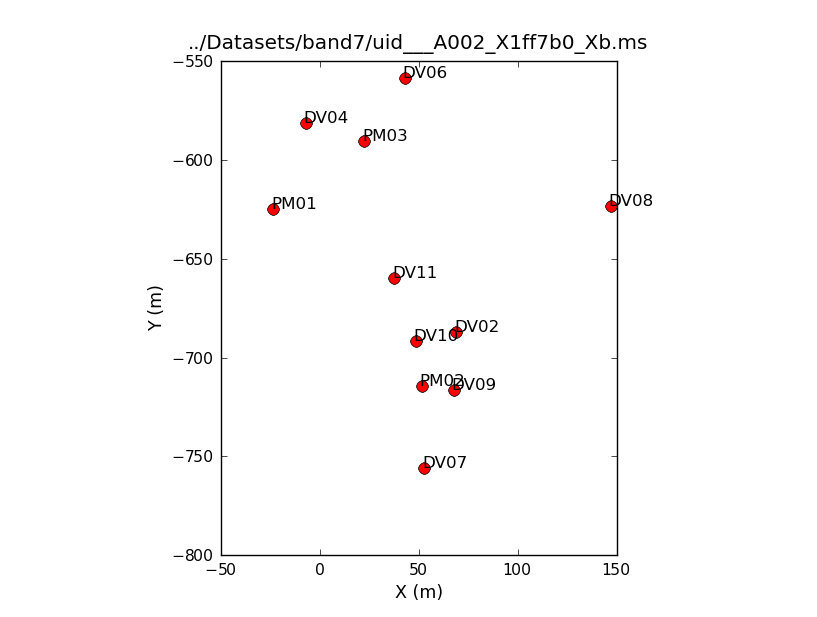
# In CASA
basename_all=["uid___A002_X1ff7b0_Xb","uid___A002_X207fe4_X3a","uid___A002_X207fe4_X3b9",
     "uid___A002_X2181fb_X49","uid___A002_X1ff7b0_X1c8","uid___A002_X207fe4_X1f7",
     "uid___A002_X207fe4_X4d7","uid___A002_X215db8_X18","uid___A002_X215db8_X1d5",
     "uid___A002_X215db8_X392"]

for asdm in basename_all:
    print "Antenna configuration for : "+asdm
    plotants(vis=asdm+'.ms', figfile=asdm+'.plotants.png')
    dummy_string = raw_input("Hit <Enter> to see the antenna configuration for the next data set.")
This will loop through all 10 data sets, show you the antenna position for each, and save that as a file named, e.g., "uid___A002_X1ff7b0_Xb.plotants.png" for the first data set. The "raw_input" command asks CASA to wait for your input before proceeding. If you would prefer to just browse the .png files after the fact you can remove this. Notice that the antenna setup changes, but only slightly, over the course of the 10 data sets.
How to Deal With 10 Measurement Sets
It should already be clear from the initial inspection that dealing with 10 data sets at the same time can be a bit problematic. This is especially tricky in our case because the Antennae data contain two distinct sets of observations: the Northern and Southern Mosaics. The source name changes between these two scripts and there are different numbers of fields in the mosaic.
As a general rule one would reduce each individual observation separately or at the very least only group data observed in a uniform way and very close in time.
Unfortunately, a CASA Guide stepping through the reduction for each of 10 data sets would quickly become unwieldy. Therefore we will use a few tricks to reduce the Antennae data in a kind of batch mode. You have already seen the first trick: we can define a python list holding the names of each data set and then loop over this list to execute the same command on each data set. For example:
# In CASA
basename_all=["uid___A002_X1ff7b0_Xb","uid___A002_X207fe4_X3a","uid___A002_X207fe4_X3b9",
     "uid___A002_X2181fb_X49","uid___A002_X1ff7b0_X1c8","uid___A002_X207fe4_X1f7",
     "uid___A002_X207fe4_X4d7","uid___A002_X215db8_X18","uid___A002_X215db8_X1d5",
     "uid___A002_X215db8_X392"]

for asdm in basename_all:
    print asdm
You only need to define your list of MS files once per CASA session. Then "basename_all" will be a variable in the casapy shell. You can check if it exists by typing "print basename_all". In the interests of allowing you to easily exit and restart CASA and pick this guide up at any point we will redefine "basename_all" in each section of the guide. Feel free to skip this step if you've already defined it in your session.
This page will step you through the reduction of the whole Antennae Band 7 SV data set using these 'for' loops. We will not be able to show every diagnostic plot but we give an example of each and the syntax to generate the rest. Also please be aware that even on a very fast machine this whole process can take a while, we are simply dealing with a lot of data.
One potential "gotcha" is that the source name changes between the two data sets. Therefore at several points we will break apart our loop to iterate separately over the Northern and Southern Mosaics, where the source can be referred unambiguously. Another subtle point is that 3c279 appears with two distinct field IDs in the Southern Mosaic, but only one in the Northern Mosaic. We will largely avoid this by referring to the source by its name but if you tried to use field ID numbers and mingled the two data sets this could cause confusion.
A Priori Flagging
Even before we look in detail, we know that there are some data that we wish to exclude. We will start by flagging "shadowed" data where one antenna blocks the line of sight of another. We will also flag scans that were used to carry out pointing and atmospheric calibration, identified by their scan intent. Finally, we'll flag the autocorrelation data (the correlation of the signal from an antenna with itself) as we are only interested in cross-correlation data to make an interferometric image.
Start by defining our list of MS files:
# In CASA
basename_all=["uid___A002_X1ff7b0_Xb","uid___A002_X207fe4_X3a","uid___A002_X207fe4_X3b9",
     "uid___A002_X2181fb_X49","uid___A002_X1ff7b0_X1c8","uid___A002_X207fe4_X1f7",
     "uid___A002_X207fe4_X4d7","uid___A002_X215db8_X18","uid___A002_X215db8_X1d5",
     "uid___A002_X215db8_X392"]
You may want to reset the flagging if you have tried this step before and are starting over though this is not necessary on your first time through. Do so using flagdata:
# In CASA
for asdm in basename_all:
    print "Reseting flags for "+asdm
    flagdata(vis=asdm+'.ms',mode='manualflag', unflag=T, flagbackup=F)
Then flag shadowed data using the command flagdata:
# In CASA
for asdm in basename_all:
    print "Flagging shadowed data for "+asdm
    flagdata(vis=asdm+'.ms',mode = 'shadow', diameter=12.0, flagbackup = F)
In the flagdata task we choose:
- vis = asdm+'.ms' : each measurement set
- mode = 'shadow',diameter=12.0: flag shadowed data, taking into account that antennas are 12m diameter
- flagbackup = F: Do not automatically back up the flag files. We will save all of the a priori flags together using flagmanager at the end of this subsection and save some space and time.
The relevant calibration information has already been extracted from the pointing and atmospheric scans and we will not need them below. Now flag the pointing scans using flagdata in 'manualflag' mode and selecting on 'intent':
# In CASA
for asdm in basename_all:
    print "Flagging calibration scans for "+asdm
    flagdata(vis=asdm+'.ms', mode='manualflag', intent='*POINTING*', flagbackup = F)
Note that because the atmospheric calibration scans contain only TDM spectral windows, they will be removed automatically when we separate out the FDM data below.
Now flag the autocorrelation data:
# In CASA
for asdm in basename_all:
    print "Flagging autocorrelation data for "+asdm
    flagdata(vis=asdm+'.ms',autocorr=True,flagbackup=F)
Finally store the current flags information using flagmanager:
# In CASA
for asdm in basename_all:
    print "Backing up 'a priori' flags for "+asdm
    flagmanager(vis = asdm+'.ms', mode = 'save', versionname = 'Apriori')
Where versionname is just the name we assign to the current flagging state in the data. We can now roll back the flags to match the current version, called 'Apriori', whenever we want. There is no reason to do this now, but the syntax would be:
# In CASA
for asdm in basename_all:
    print "Resorting up 'a priori' flags for "+asdm
    flagmanager(vis = asdm+'.ms', mode = 'restore', versionname = 'Apriori')
It would have been possible to set flagdata to flagbackup=T so that it stores the flags at each of the flagging step automatically, but this way it is a bit more efficient with regard to time and disk space. More important, lumping all the a priori flagging together gives us a natural point to roll back to if we get in trouble.
The flagmanager task will also allow you to view the saved flagging versions,
including those created by running flagdata with flagbackup=T.

For example try

flagmanager(vis='uid___A002_X2181fb_X49.ms', mode='list')

The output in the logger should list the Apriori flagging that we have applied.
It will also indicate versions associated with any flagdata command where you
did not set flagbackup=F. Other tasks, for example applycal, will also create
flag version tables.
Examine and Apply Tsys, WVR, and Antenna Position Calibration Tables Then Split
The Antennae_Band7_UnCalibratedMSandTablesForReduction directory includes system temperature (Tsys), water vapor radiometer (WVR), and antenna position calibration tables, which appear as files with extensions '.tsys.cal.fdm', '.wvr.cal', and '.antpos'. The WVR and Tsys tables have been built from the spw 0 (WVR) and spw 5 & 7 (Tsys) data. We provide these to you because CASA does not generate them at the moment, a situation that will change soon. The Tsys calibration gives a first-order correction for the atmospheric opacity as a function of time and frequency and associates weights with each visibility that persists through imaging. The WVR calibration uses observations of the wings of the 183 GHz atmospheric water line to correct for phase variations as a function of time. The antenna position table reflects refinements in the measured positions of the antennas from those stored in the data.
We inspect the Tsys tables for the spectral window spw=1 with the task plotcal. We want to check that Tsys data have reasonable values and identify any unexpected features as a function of either time or frequency. To get an idea of sensible Tsys under average atmospheric observations consult the ALMA sensitivity calculator, accessible from http://www.almascience.org .
We start by plotting the Tsys for all the antennas and polarizations (XX and YY) as a function of time for each. Here and throughout we focus on spw 1, which contains CO(3-2):
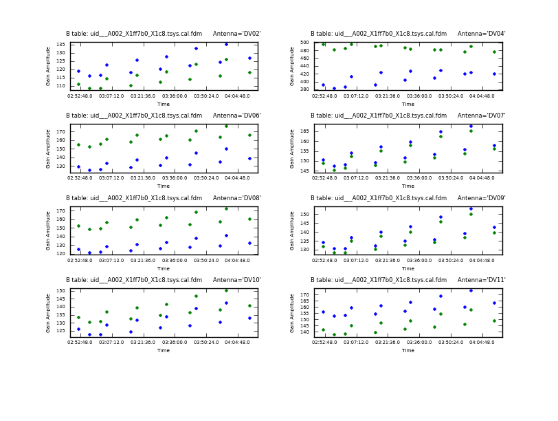
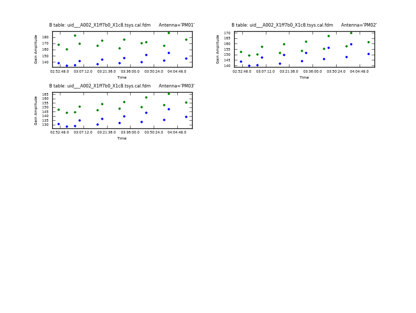
#In CASA
basename_all=["uid___A002_X1ff7b0_Xb","uid___A002_X207fe4_X3a","uid___A002_X207fe4_X3b9",
     "uid___A002_X2181fb_X49","uid___A002_X1ff7b0_X1c8","uid___A002_X207fe4_X1f7",
     "uid___A002_X207fe4_X4d7","uid___A002_X215db8_X18","uid___A002_X215db8_X1d5",
     "uid___A002_X215db8_X392"]


for asdm in basename_all:
    print "Plotting Tsys vs. time for "+asdm
    plotcal(caltable=asdm+'.tsys.cal.fdm',
	    xaxis="time",yaxis="amp",
	    spw='1:1200~1200',plotsymbol=".", subplot=421,
	    antenna='0~7',
	    iteration='antenna', figfile=asdm+'.tsys_vs_time.page1.png',
	    fontsize=6.0)
    #dummy_string = raw_input("First eight antennas for "+asdm+" . Hit <Enter> to continue.")
    plotcal(caltable=asdm+'.tsys.cal.fdm',
	    xaxis="time",yaxis="amp",
	    antenna='8~15',
	    spw='1:1200~1200',plotsymbol=".", subplot=421,
	    iteration='antenna', figfile=asdm+'.tsys_vs_time.page2.png',
	    fontsize=6.0)
    #dummy_string = raw_input("Remaining antennas for "+asdm+" . Hit <Enter> to continue.")
This sequence loops over all of our files and plots Tsys as a function of time for channel 1200 in spectral window 1. In the call to plotcal:
- subplot=421 parameter sets up a 4 x 2 panel grid.
- iteration tells plotcal to make a separate plot for each antenna.
- spw '1:1200~1200' selects spw '1' channel 1200-1200. This allows us to cleanly separate time variations from frequency variations.
Because 8 panels is not enough to show all antennas on one page, there are two plotcal calls: one for the first 8 antennas (antenna=0~7) and one for any remaining antennas (antenna=8~15). The fontsize needs to be set to a small value or the text overlaps.
The 'raw_input' commands will wait for you to hit Enter before issuing the next plot command. In the example above these are commented out (the leading "#" means that CASA will ignore them). If you would like to interactively cycle through the plots, uncomment them by removing the "#". Otherwise, the figfile parameter directs the output to .png files for later inspection. The easiest way to look at the 20 plots produced here is to simply inspect the .png files using your favorite viewer.
The Tsys values in Figure 2 look reliable, with typical values ~150 K except for some large values of Tsys at ~300 and 400 K for DV04. We will flag the data for that antenna later.
We will also want to look at Tsys as a function of frequency. The following commands step through how you would do this, but do not execute this command blindly! (just in case, we have included a "break" that you will need to remove before running or the "for" loop will simply cancel). The commands are similar to the Tsys vs. time plotcal but will take much longer to run because instead of tracking a single channel we now plot the data for all 3840 channels in spw 1. Future enhancements to CASA will make it possible to plot these data more efficiently (e.g., by stepping across channels) but for now it takes a long time to generate these plots. We have included them in the directory "tsys_plots/" in the distribution you downloaded so that you will not need to generate them yourself. If you really want to run this command, remove the "break" and run the commands:
#In CASA

for asdm in basename_all:
    break
    print "Plotting Tsys vs. frequency for "+asdm
    plotcal(caltable=asdm+'.tsys.cal.fdm',
	    xaxis="freq",yaxis="amp",
	    spw='1', plotsymbol=".", subplot=421,
	    iteration='antenna', figfile=asdm+'.tsys_vs_freq.page1.png',
	    antenna='0~7', fontsize=6.0)
    #dummy_string = raw_input("Inspecting Tsys table for "+asdm+" . Hit <Enter> to continue.")
    plotcal(caltable=asdm+'.tsys.cal.fdm',
	    xaxis="freq",yaxis="amp",
	    spw='1', plotsymbol=".", subplot=421,
	    iteration='antenna', figfile=asdm+'.tsys_vs_freq.page2.png',
	    antenna='8~15', fontsize=6.0)
    #dummy_string = raw_input("Inspecting Tsys table for "+asdm+" . Hit <Enter> to continue.")
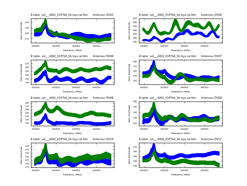
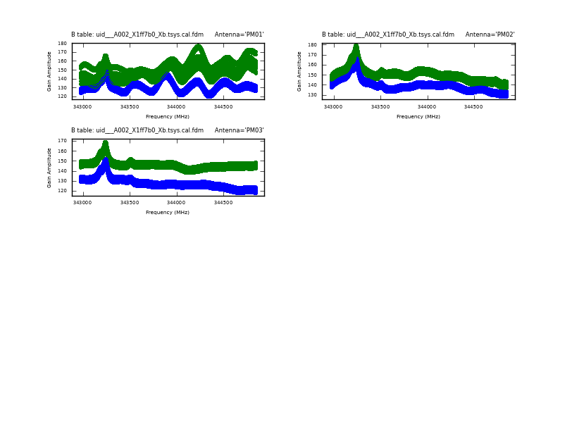
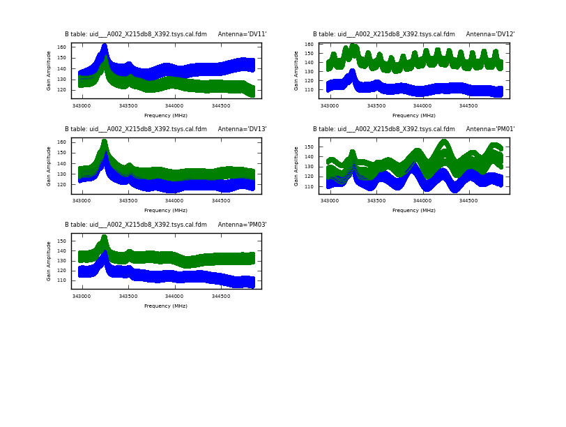
Now have a look at the Tsys vs. frequency plots or see Figure 3 for an example on the first data set. You can see the effect of a close pair of atmospheric ozone absorption lines at about 343.2 GHz that makes Tsys larger near that frequency in all antennas. Applying the Tsys calibration tables will minimize the contribution of these atmospheric lines. Again DV04 stands out with its very high Tsys. Although not present in the first data sets, Antenna DV12 exhibits periodic spikes in Tsys vs. frequency for one polarization (see Figure 3c for an example from a later data set). It may or may not be possible to calibrate that behavior out. We will make a note to look carefully at DV12 further on in the calibration process.
We are now ready to apply the Tsys and the WVR calibration tables to the data with applycal, which reads the specified gain calibration tables, applies them to the (raw) data column, and writes the calibrated results into the corrected column. Again, we loop through all the datasets. It is important to only apply Tsys and WVR corrections obtained close in time to the data being corrected, so in addition to looping over data sets we define the list of unique source names and loop over these. Then by setting gainfield and field to the same value we ensure that Tsys and WVR calibrations are only applied to the source for which they are measured. Because the source has a different name in the Northern Mosaic and the Southern Mosaic, we will carry out two loops. We will only correct spw 1, our science window, because we will drop the other data in a moment.
# In CASA

# A new list of file names that contain only data from the Northern Mosaic
basename_north=["uid___A002_X1ff7b0_Xb","uid___A002_X207fe4_X3a","uid___A002_X207fe4_X3b9","uid___A002_X2181fb_X49"]
field_names_north = ['Titan','3c279','NGC*']

for asdm in basename_north:
    print "Apply Tsys, WVR, and Antenna Position calibrations to "+asdm
    for field in field_names_north:
        applycal(vis=asdm+".ms", spw='1',
            field=field, gainfield=["",field,field],
            interp='nearest',
            gaintable=[asdm+".antpos",asdm+".tsys.cal.fdm",asdm+'.wvr.cal'],
            flagbackup=F)

# A new list of file names that contain only data from the Southern Mosaic
basename_south=["uid___A002_X1ff7b0_X1c8","uid___A002_X207fe4_X1f7","uid___A002_X207fe4_X4d7",
                           "uid___A002_X215db8_X18","uid___A002_X215db8_X1d5","uid___A002_X215db8_X392"]
field_names_south = ['Titan','3c279','Ant*']

for asdm in basename_south:
    print "Apply Tsys, WVR, and Antenna Position calibrations to "+asdm
    for field in field_names_south:
        applycal(vis=asdm+".ms", spw='1',
            field=field, gainfield=["",field,field],
            interp='nearest',
            gaintable=[asdm+".antpos",asdm+".tsys.cal.fdm",asdm+'.wvr.cal'],
            flagbackup=F)
where:
- field: the field to which we will apply the calibration,
- gainfield: the field from which we wish to take the calibration table
- interp = 'nearest' : apply the nearest solution from the calibration table rather than interpolating.
As you browse through the whole data set, you will probably note some problems along the same lines as the DV04 issue we saw above. We'll apply these as additional data flagging in just a moment. First, with the Tsys and WVR calibrations applied successfully and the a priori flagging taken care of we will now split out the corrected data. We will keep only the corrected data, specified via datacolumn, and only spectral window 1, which contains the FDM (high spectral resolution) observations of the CO(3-2) line. Setting keepflags=F tells split not to carry over any fully flagged rows from the original data set to the new MS. We give the new MS files the extension ".wvrtsys.ms" to indicate that they have been corrected for WVR and Tsys effects. Because split will not overwrite existing files, we remove any previous versions of the new MS before beginning.
# In CASA
for asdm in basename_all:
    os.system('rm -rf '+asdm+'.wvrtsys.ms')
    print "Splitting out corrected data for "+asdm
    split(vis=asdm+'.ms', outputvis=asdm+'.wvrtsys.ms',
        datacolumn='corrected', spw='1', keepflags=F)
Be patient, split may take awhile. The WVR and Tsys-corrected data now sit in the DATA column of the new measurement sets, which have only one spectral window (now labeled spectral window 0 though it was spectral window 1 in the original data). You may wish to run listobs to illustrate the changes:
# In CASA
for asdm in basename_all:
    os.system('rm '+asdm+'.wvrtsys.listobs.txt')
    listobs(vis=asdm+'.wvrtsys.ms', listfile=asdm+'.wvrtsys.listobs.txt', verbose=True)
Note the new spectral window information:
2011-08-05 01:07:08 INFO listobs	Spectral Windows:  (1 unique spectral windows and 1 unique polarization setups)
2011-08-05 01:07:08 INFO listobs	  SpwID  #Chans Frame Ch1(MHz)    ChanWid(kHz)TotBW(kHz)  Ref(MHz)    Corrs
2011-08-05 01:07:08 INFO listobs	  0        3840 TOPO  344845.586  488.28125   1875000     344908.33   XX  YY
Inspect Data
We are not quite done with the original ".ms" data sets yet. Before going further it will be useful to use plotms to show the effects of applying the calibration. In the process we'll take a quick look at each antenna and search for pathologies in the data.
For this basic inspection, we want to compare the phase and amplitude as a function of frequency and time in the DATA and CORRECTED columns of each measurement set. The CORRECTED column has had the Tsys and WVR calibrations applied and so we expect lower phase scatter and flatter amplitude response as a function of time and frequency. We are looking for antenna-based issues, so cycling through a set of baselines that includes each antenna once will be a good start. We'll focus these plots on the phase+bandpass calibrator, 3c279, and on baselines that include antenna DV11, which we will make our reference antenna in just a bit.
Each CASA Measurement Set has up to three "columns" of data: DATA, CORRECTED, and MODEL (though it is possible
for a MS to hold only a DATA column if it has not been processed at all).

A column entry exists for each data point (baseline, frequency, time).

The DATA column holds the current raw data, though using split as we just did we can change the definition of
"raw" data.

The CORRECTED column holds the result of applying one or more calibration tables (e.g., via applycal) to the
DATA column and so represents a corrected version of the DATA column.

The MODEL column holds an external estimate of what the visibilities should be for that data point. We will
set this using the task setjy, which includes a model of Titan, and during imaging.

To get an intuitive feel for the columns you may wish to explore using plotms (which can plot different data
columns, as seen below) or the browsetable task.
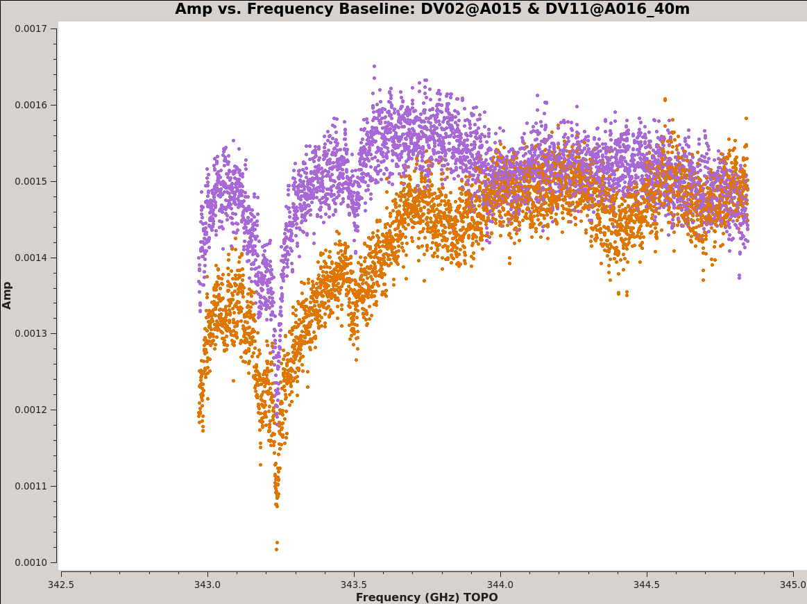
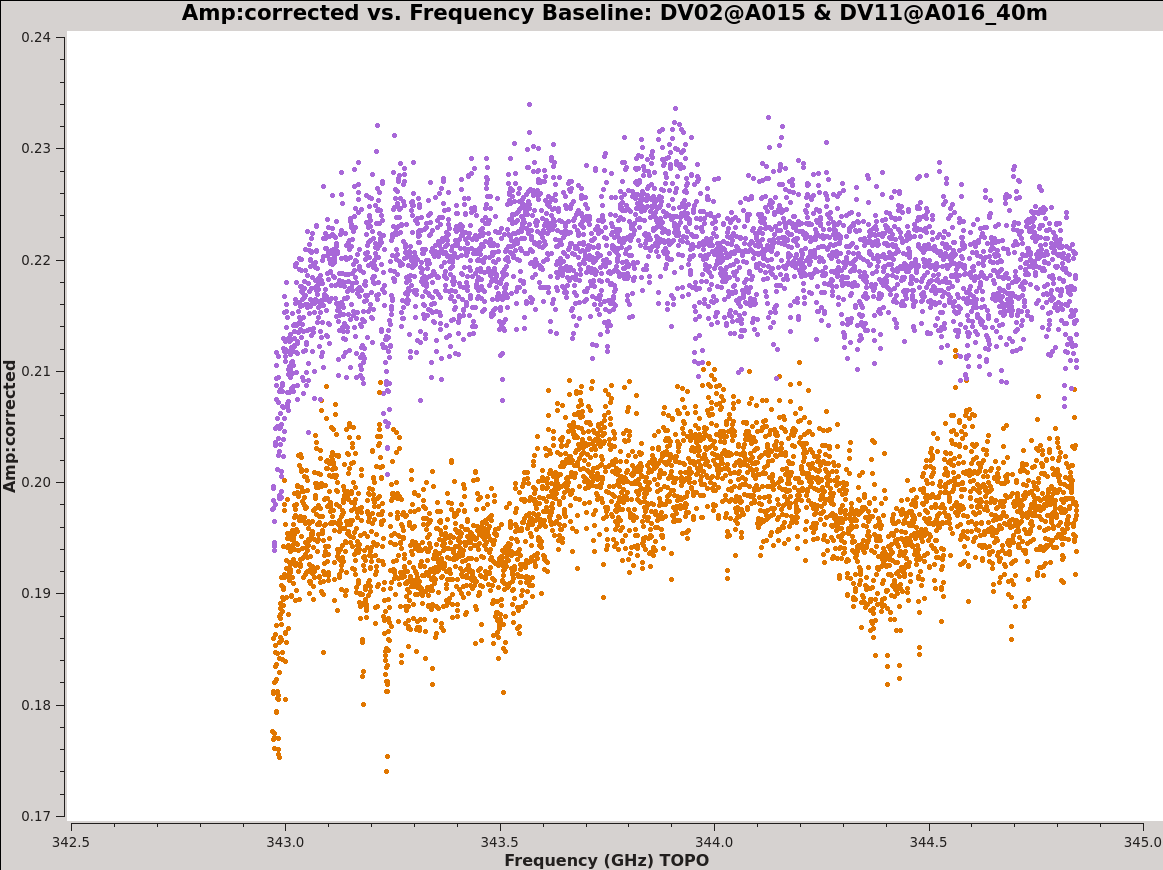
First, we plot amplitude as a function of frequency for 3c279. We start by plotting the DATA column, set color to indicate the two correlations (i.e., the XX and YY polarizations), and ask plotms to iterate over baseline. By setting antenna to 'DV11&*' we select only baselines that include DV11. We ask plotms to average all data over a very long timescale, avgtime = 1e8 seconds ~ 3 years or much longer than the time spanned by the whole data set. By setting avgscan = True we allow plotms to average across scan boundaries. The result is a plot of average amplitude per channel vs. frequency.
# In CASA
basename_all=["uid___A002_X1ff7b0_Xb","uid___A002_X207fe4_X3a","uid___A002_X207fe4_X3b9",
     "uid___A002_X2181fb_X49","uid___A002_X1ff7b0_X1c8","uid___A002_X207fe4_X1f7",
     "uid___A002_X207fe4_X4d7","uid___A002_X215db8_X18","uid___A002_X215db8_X1d5",
     "uid___A002_X215db8_X392"]

asdm=basename_all[0]

plotms(vis=asdm+'.ms',
       field='3c279',
       xaxis='frequency', yaxis='amp',
       selectdata=T, spw='1',
       avgtime='1e8',avgscan=T,
       coloraxis='corr',
       iteraxis='baseline',
       antenna='DV11&*',
       ydatacolumn='data')
Notice the green arrows along the bottom of the plotms window. We asked plotms to iterate over baseline. As you click the arrows, the plot will rotate from baseline to baseline, always with DV11 so that each antenna shows up once. To see the effect of the calibration, go to the "Axes" tab along the left of the plotms window and pull down the Data Column menu under the Y Axis. Set this from DATA to CORRECTED and you should see the effects of the calibration. You may need to ensure that the "Force Reload" box is checked before clicking "Plot" (both buttons lie at the bottom of the panel). For the most part things get better (flatter), but as we noted before DV04 is problematic.
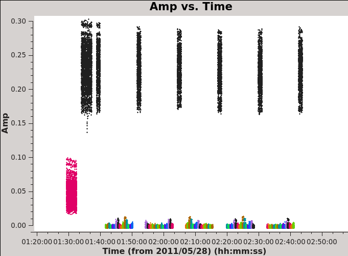
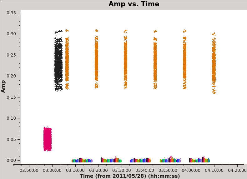
You can now make analogous calls to examine the phase vs. frequency, amplitude vs. time, and phase vs. time.
# In CASA

plotms(vis=asdm+'.ms',
       field='3c279',
       xaxis='frequency', yaxis='phase',
       selectdata=T, spw='1',
       avgtime='1e8',avgscan=T,
       coloraxis='corr',
       iteraxis='baseline',
       antenna='DV11&*',
       ydatacolumn='data')

plotms(vis=asdm+'.ms',
       field='3c279',
       xaxis='time', yaxis='amp',
       selectdata=T, spw='1:1200~1300',
       avgchannel='1000',avgscan=F,
       coloraxis='corr',
       iteraxis='baseline',
       antenna='DV11&*',
       ydatacolumn='data')

plotms(vis=asdm+'.ms',
       field='3c279',
       xaxis='time', yaxis='phase',
       selectdata=T, spw='1:1200~1300',
       avgchannel='1000',avgscan=F,
       coloraxis='corr',
       iteraxis='baseline',
       antenna='DV11&*',
       ydatacolumn='data')
Where:
- spw is set to cover only channels 1200~1300 for the time plots in order to isolate time dependent variations from frequency-dependent behavior. Those 101 channels represent only a small part of the total spw 1 bandpass.
- avgchannel set to a large number causes the plots of phase and amplitude vs. time to average data at all frequencies into a single point for each measurement.
- coloraxis corr sets the colors to correspond to the two polarizations of the data.
In each case, you will want to examine each baseline, alternating between the DATA and CORRECTED columns.
This is a lot of data inspection and that's only for one of 10 data sets! You can iterate across the data by hand, updating "asdm" to refer to each data set in order and cycling between baselines and DATA/CORRECTED. It is also possible to script CASA to show you the key plots in succession (see the next block down). However you approach the infrastructure, you are looking for:
- Improved scatter and lower variability in phase and amplitude vs. frequency and time. This indicates that the WVR and Tsys calibrations helped.
- Sudden jumps in phase or amplitude as a function of either time or frequency. These may indicate problems with the antenna during that observation.
- Large gradients, especially full wraps, in phase as a function of frequency. This may indicate a problem in the delays, the signal path length to the telescopes.
- Unusual magnitude, scatter, or patterns in any plot - though this may be better explored using plots that show all data together, which we'll make in a moment.
- Missing data. For example, if the phase calibrator drops out for a period of time we will not be able to calibrate and will need to flag the data.
As you look through, note individual potentially problematic antennas. If all antennas in a data set appear problematic it may be that your "reference" antenna, DV11 in the example above, is the source of the problem. In this case swap this reference antenna for another and see whether the problem is isolated to your original reference antenna.
A brief aside on structure:

This section (Data Inspection) and the next (Apply Flags) are closely linked. We will present them as two
separate steps. The idea here is that you look through your data, note problems, and then write commands to
flag problematic data. This mimics one approach to writing data reduction scripts for CASA, where you will
group all flagging together into one convenient place. Other CASA guides take a different approach, interleaving flagging and plotting. There is no "right" answer here. Find an approach to data inspection
that works for you.
If you do wish to semi-automate the plot generation, the following sequence will cycle between data and corrected plots for each data set in turn. Type "stop" at any input call to break out.
# In CASA

user_input = ""
for asdm in basename_all:
    # check if a stop has been requested
    if user_input == "stop":
        break
    # Extract antenna list for this data set.
    tb.open(asdm+'.ms/ANTENNA', nomodify=True)
    ants = tb.getcol('NAME')
    tb.close
    # Define the reference antenna to make baselines with
    ref_ant = 'DV11'
    # Loop over antennas
    for ant in ants:
        # Check if the user wants to stop
        if user_input == "stop":
            break
        # Skip correlation of reference antenna with itself (autocorrelations are flagged anyhow)
        if ant == ref_ant:
            continue
        # Define the baseline with the reference antenna for current antenna
        ant_str = ref_ant+'&'+ant
        print "Showing baseline "+ant_str+" for data set "+asdm
        print "Use this to inspect effect of applying wvrcal and Tsys calibrations."
        # Loop over phase and amplitude as axes
        for y_axis in ["amp", "phase"]:
            # Make 'before' plot for frequency x-axis
            print "... "+y_axis+" vs. frequency for DATA:"
            plotms(vis=asdm+'.ms', spw='1', field='3c279',
               antenna=ant_str, xaxis="frequency", yaxis=y_axis,
               avgtime="1e8", avgscan=T, coloraxis="corr",
               ydatacolumn="data")
            user_input = raw_input("Hit <ENTER> to see CORRECTED data [type 'stop'+<Enter> to break out].")
            if user_input == "stop":
                break
            # Make 'after' plot for frequency x-axis
            print "... "+y_axis+" vs. frequency for CORRECTED:"
            plotms(vis=asdm+'.ms', spw='1', field='3c279',
               antenna=ant_str, xaxis="frequency", yaxis=y_axis,
               avgtime="1e8", avgscan=T, coloraxis="corr",
               ydatacolumn="corrected")
            user_input = raw_input("Hit <ENTER> to proceed to next plot [type 'stop'+<Enter> to break out].")
            if user_input == "stop":
                break
            # Make 'before' plot for time x-axis
            print "... "+y_axis+" vs. time for DATA:"
            plotms(vis=asdm+'.ms', spw='1:1200~1300', field='3c279',
               antenna=ant_str, xaxis="time", yaxis=y_axis,
               avgchannel="1000", coloraxis="corr",
               ydatacolumn="data")
            user_input = raw_input("Hit <ENTER> to see CORRECTED data [type 'stop'+<Enter> to break out].")
            if user_input == "stop":
                break
            # Make 'after' plot for time y-axis
            print "... "+y_axis+" vs. time for CORRECTED:"
            plotms(vis=asdm+'.ms', spw='1:1200~1300', field='3c279',
               antenna=ant_str, xaxis="time", yaxis=y_axis,
               avgchannel="1000", coloraxis="corr",
               ydatacolumn="corrected")
            user_input = raw_input("Hit <ENTER> to proceed to next plot [type 'stop'+<Enter> to break out].")
            if user_input == "stop":
                break
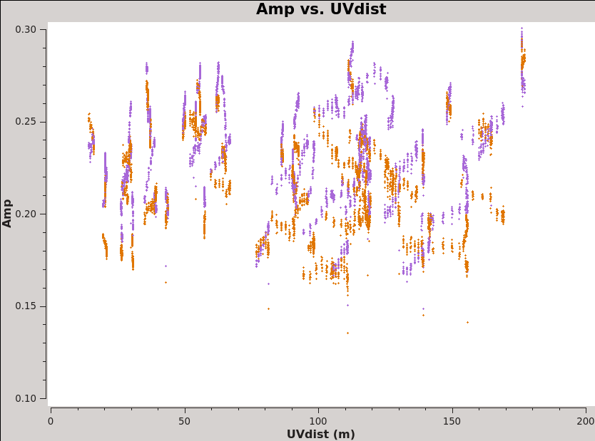
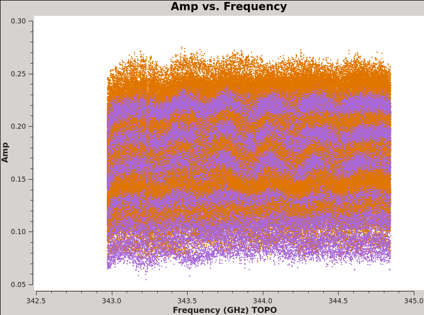
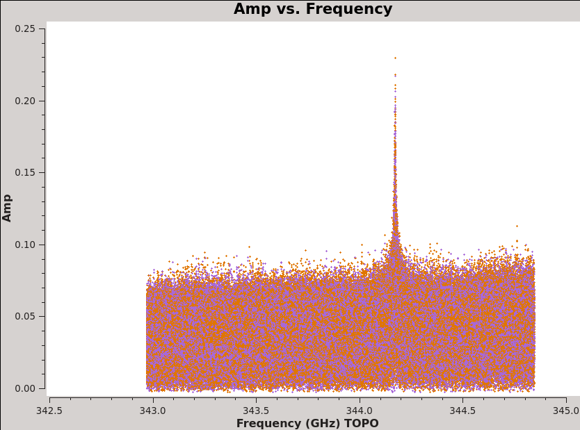
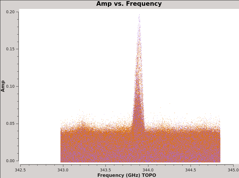
A detailed explanation of the procedure is a bit outside the scope of this guide (for more on python see http://www.python.org/ and for more on the CASA toolkit see http://casa.nrao.edu/), but the basic process is to loop over each data set, baseline with the reference antenna (here DV11), and y-axis of interest (phase or amplitude) then plot the effect of the calibration vs. frequency and time for each combination. Running this to step through the data will give you about 200 "before and after" plots from which you could note a subset of problematic cases to be followed up by hand. Many other strategies to inspect the data are also viable.
Next we will do a bit more inspection using plotms to look at whole data sets. This will help us identify missing data or look for egregious outliers.
First we plot amplitude versus time (see Figure 5), averaging over all channels (by setting avgchannel to the very large value 10,000). We colorize by field so that scans on Titan are red, the bandpass and phase calibrator 3c279 is black (and orange in the Southern Mosaic where it has two field IDs), and the Antennae mosaic appears as a range of colors (one per pointing).
# In CASA
for asdm in basename_all:
    plotms(vis=asdm+'.wvrtsys.ms',
            xaxis='time', yaxis='amp',
            avgchannel='10000',coloraxis='field')
    dummy_string = raw_input("Examining amplitude vs. time for "+asdm+" . Hit <Enter> to proceed.")
Here look for:
- Missing data. The source needs to be flanked by phase calibrator scans, if those are missing for any reason we need to flag the appropriate time range.
- Dramatic outliers. Does the source suddenly get very bright or the otherwise bright calibrator appear anomalously faint for a brief time? This likely indicates problematic data that should be identified and flagged. You can use the "select" (box with green plus along the bottom row in plotms) and "locate" (magnifying glass) buttons in plotms to isolate and identify problem data (it will print to the log).
- Smooth variation with time. A sudden jump may indicate a problem and often the safest approach is to flag data near a discontinuity.
Look through the amplitudes vs. time for each data set (remember that we've already examined the phases vs. time and amplitude vs. time for individual baselines above).
There are two other very useful "averaging" plots worth making. First, we plot amplitude as a function of u-v distance (projected antenna separation). Discontinuities and spikes in this plot are often from non-astrophysical sources. In the phase analog to the plot, the effects of atmospheric decorrelation can be assessed from increased scatter at longer u-v distances. While using the moon Titan as our flux calibrator, we may want to watch for flaring amplitudes at short u-v distances. These may indicate that Saturn is contaminating our beam. For a perfect, bright point source, we expect flat amplitudes as a function of u-v distance at the source amplitudes. Figure 6 shows an example of this plot, generated via:
# In CASA
for asdm in basename_all:
    plotms(vis=asdm+'.wvrtsys.ms',
        field='3c279',
        xaxis='uvdist', yaxis='amp',
        avgchannel='10000',coloraxis='corr')
    dummy_string = raw_input("Examining amplitude vs. time for 3c279 for "+asdm+" . Hit <Enter> to proceed.")
    plotms(vis=asdm+'.wvrtsys.ms',
        field='Titan',
        xaxis='uvdist', yaxis='amp',
        avgchannel='10000',coloraxis='corr')
    dummy_string = raw_input("Examining amplitude vs. time for Titan for "+asdm+" . Hit <Enter> to proceed.")
It can also be useful to examine the average amplitude as a function of frequency for each target. This allows one to check for lingering atmospheric effects, unexpected line emission or absorption in the calibrators, or decreased sensitivity due to "roll-off" of the telescope sensitivity at the band edges. These plots are created by the sequence of commands below, where we have broken up the script to loop separately over the Northern and Southern Mosaics to reflect the different source names.
# In CASA

basename_north=["uid___A002_X1ff7b0_Xb","uid___A002_X207fe4_X3a","uid___A002_X207fe4_X3b9","uid___A002_X2181fb_X49"]

field_names = ["3c279","Titan","NGC*"]

for asdm in basename_north:
    for field in field_names:
        plotms(vis=asdm+'.wvrtsys.ms',
            field=field,
            xaxis='frequency', yaxis='amp',
            avgtime='1e8',avgscan=T, coloraxis='corr')
        dummy_string = raw_input("Examining amplitude vs. frequency for "+field+" in "+asdm+" . Hit <Enter> to proceed.")

basename_south=["uid___A002_X1ff7b0_X1c8","uid___A002_X207fe4_X1f7","uid___A002_X207fe4_X4d7",
                           "uid___A002_X215db8_X18","uid___A002_X215db8_X1d5","uid___A002_X215db8_X392"]

field_names = ["3c279","Titan","Ant*"]

for asdm in basename_south:
    for field in field_names:
        plotms(vis=asdm+'.wvrtsys.ms',
            field=field,
            xaxis='frequency', yaxis='amp',
            avgtime='1e8',avgscan=T, coloraxis='corr')
        dummy_string = raw_input("Examining amplitude vs. frequency for "+field+" in "+asdm+" . Hit <Enter> to proceed.")
For this command notice that we can see the CO(3-2) line in the Antennae even before calibration (see Figure 7) and that Titan also shows evidence of a strong line (also Figure 7)! This will need to be flagged before we can use Titan to calibrate the flux scale of our data.
This suite of plots (along with the earlier inspection of the Tsys tables) gives us the tools we need to identify problematic data through the data sets. We use this to generate a set of inspection-driven flagdata commands for each data set. We apply these before the bandpass and gain calibration.
Apply Flagging
Based on this inspection and the other plots we have made, we now flag problematic portions of the data. We break up the flags by reason for flagging in order to illustrate the process. As you reduce your own data it may be more efficient to group flags by data set and make use of the flagcmd command. Except for the "post-calibration" flagging, the inspection plots that we just looked through have already revealed all of the problems that we flag. We structure the guide so that the flagging is grouped in one place.
As before, we may wish to reset our flags before beginning (particularly if one iterates this process) via:
# In CASA

basename_all=["uid___A002_X1ff7b0_Xb","uid___A002_X207fe4_X3a","uid___A002_X207fe4_X3b9",
     "uid___A002_X2181fb_X49","uid___A002_X1ff7b0_X1c8","uid___A002_X207fe4_X1f7",
     "uid___A002_X207fe4_X4d7","uid___A002_X215db8_X18","uid___A002_X215db8_X1d5",
     "uid___A002_X215db8_X392"]

for asdm in basename_all:
    flagdata(vis = asdm+'.wvrtsys.ms',mode='manualflag', unflag= T, flagbackup = F)
Remember that we dropped the flagged data when splitting out after the WVR and Tsys calibration, so this should not undo your "A Priori" flagging of shadowed data, autocorrelations, etc.. In any case this unflagging step is not necessary during the first iteration.
- Edge Channels
ALMA's sensitivity decreases near the edge of the baseband and it is often useful to check for a 'roll-off' in sensitivity near the edge of the band. This will appear as a downturn in amplitude as a function of channel near the edge of the window in the uncalibrated data, as a flaring due to increased noise at the spw edges in the calibrated data. It will also be visible in the amplitude part of the bandpass calibration table. Because our FDM spw does not cover the full baseband, we do not see a strong roll off in our data (see Figure 8a), where there is only a mild hint of a roll-off at the high end) but we do flag a (very) few channels at the high and low-frequency edge of the data set to be safe.
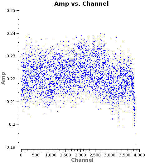
# In CASA

for asdm in basename_all:
    flagdata(vis = asdm+'.wvrtsys.ms',spw = '0:0~7,0:3831~3839', flagbackup = F)
- Problematic Tsys measurements
Above we noted issues with the Tsys measurements for both DV04 and DV12. We flag the affected data. Each of these issues should be visible in the Tsys plots you made above (e.g., see Figure 3).
# In CASA

asdm="uid___A002_X1ff7b0_Xb"
flagdata(vis=asdm+'.wvrtsys.ms', mode='manualflag',antenna='DV04', flagbackup=F)

asdm="uid___A002_X207fe4_X3a"
flagdata(vis=asdm+'.wvrtsys.ms',antenna='DV12',correlation='YY', flagbackup=F)

asdm="uid___A002_X207fe4_X3b9"
flagdata(vis=asdm+'.wvrtsys.ms',antenna='DV12',correlation='YY', flagbackup=F)

asdm="uid___A002_X2181fb_X49"
flagdata(vis=asdm+'.wvrtsys.ms',antenna='DV12',correlation='YY', flagbackup=F)

asdm="uid___A002_X1ff7b0_X1c8"
flagdata(vis=asdm+'.wvrtsys.ms',antenna='DV04',flagbackup=F)

asdm="uid___A002_X207fe4_X1f7"
flagdata(vis=asdm+'.wvrtsys.ms',antenna='DV12',correlation='YY', flagbackup=F)

asdm="uid___A002_X207fe4_X4d7"
flagdata(vis=asdm+'.wvrtsys.ms',antenna='DV12',correlation='YY', flagbackup=F)

asdm="uid___A002_X215db8_X18"
flagdata(vis=asdm+'.wvrtsys.ms',antenna='DV12',correlation='YY', flagbackup=F)

asdm="uid___A002_X215db8_X1d5"
flagdata(vis=asdm+'.wvrtsys.ms',antenna='DV12',correlation='YY', flagbackup=F)

asdm="uid___A002_X215db8_X392"
flagdata(vis=asdm+'.wvrtsys.ms',antenna='DV12',correlation='YY', flagbackup=F)
- Unreliable Short-Spacing Measurements on Titan
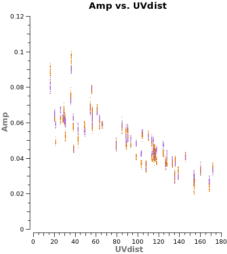
Saturn may contaminate the short u-v spacings from Titan. In any case these often show significant scatter (Figure 8b), so we flag them. There are still enough baselines to determine a good amplitude calibration for each antenna.
# In CASA

asdm="uid___A002_X1ff7b0_Xb"
flagdata(vis=asdm+'.wvrtsys.ms', mode='manualflag', field='Titan', uvrange='0~50', flagbackup = F)

asdm="uid___A002_X207fe4_X3a"
flagdata(vis=asdm+'.wvrtsys.ms', mode='manualflag', field='Titan', uvrange='0~40', flagbackup = F)

asdm="uid___A002_X207fe4_X3b9"
flagdata(vis=asdm+'.wvrtsys.ms', mode='manualflag', field='Titan', uvrange='0~50', flagbackup = F)

asdm="uid___A002_X2181fb_X49"
flagdata(vis=asdm+'.wvrtsys.ms', mode='manualflag', field='Titan', uvrange='0~30', flagbackup = F)

asdm="uid___A002_X1ff7b0_X1c8"
flagdata(vis=asdm+'.wvrtsys.ms', mode='manualflag', field='Titan', uvrange='0~50', flagbackup = F)

asdm="uid___A002_X207fe4_X1f7"
flagdata(vis=asdm+'.wvrtsys.ms', mode='manualflag', field='Titan', uvrange='0~30', flagbackup = F)

asdm="uid___A002_X207fe4_X4d7"
flagdata(vis=asdm+'.wvrtsys.ms', mode='manualflag', field='Titan', uvrange='0~30', flagbackup = F)
- Delay Issues
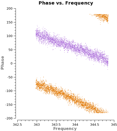
DV13 and a few other antennas show signatures of an imperfect delay calibration. This is most easily identified via strong "wrapping" of phase as a function of frequency. Such effects can be calibrated out with mild delay issues largely accounted for by the bandpass solution. The phase wrapping in DV13 seems weak enough that we will trust the calibrations to remove it. For a more extreme example see the CASA guide describing the calibration of NGC3256Band3.
- Missing Phase Calibrator Observations
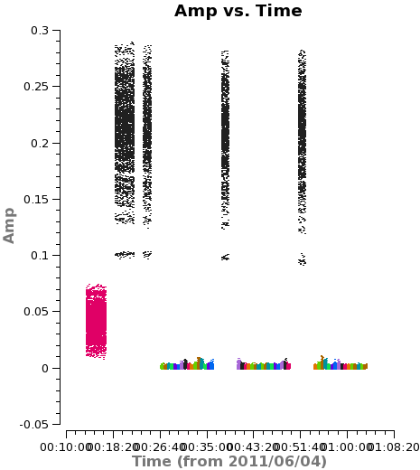
As a general rule, we want to be sure that observations of the phase calibrator (3c279) bracket each source observation. Two of the data sets do not include a final phase calibrator observation (see Figure 10) and for those two cases we flag the affected source observations.
# In CASA

asdm="uid___A002_X207fe4_X3b9"
flagdata(vis=asdm+'.wvrtsys.ms',mode='manualflag',timerange='00:53:47~01:08:00',flagbackup = F)

asdm="uid___A002_X215db8_X18"
flagdata(vis=asdm+'.wvrtsys.ms',mode='manualflag',antenna='DV10',timerange='19:46:20~20:34:40',flagbackup=F)
- Unexpected Scatter or Discontinuity in the Data
For several antennas we find sudden jumps in the phase of the phase calibrator as a function of time, these are visible in the plots of uncalibrated phase vs. time for single baselines above and we show an example in Figure 11. It will not be possible to effectively interpolate the phase between measurements when we see these discontinuities. The safest approach is to flag the source data across these jumps. We do so here (though note that the last two flaggings are borderline cases).
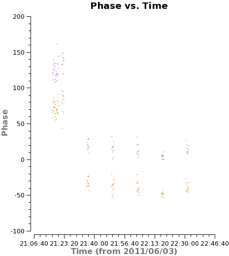
# In CASA

asdm="uid___A002_X207fe4_X3a"
flagdata(vis=asdm+'.wvrtsys.ms',mode='manualflag',antenna='DV09', timerange='21:24:09~21:35:35', flagbackup = F)

asdm="uid___A002_X207fe4_X1f7"
flagdata(vis=asdm+'.wvrtsys.ms',mode='manualflag',antenna='DV09',timerange='23:30:52~24:10:00',flagbackup=F)
flagdata(vis=asdm+'.wvrtsys.ms',mode='manualflag',antenna='PM01',timerange='23:16:50~24:10:00',flagbackup=F)
flagdata(vis=asdm+'.wvrtsys.ms',mode='manualflag',antenna='PM03',timerange='23:16:50~24:10:00',flagbackup=F)
- Outliers Visible After Calibration
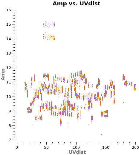
Often issues with the data may become evident after calibration (i.e., after the next few steps that we apply). These data can appear as outliers in diagnostic plots for the calibrated data or even show up in the imaging stages. Once these are identified, best practice is to apply this new flagging then redo the calibration (if the issue is very minor, then re-calibrating may not be necessary).
# In CASA
asdm="uid___A002_X207fe4_X3a"
flagdata(vis=asdm+'.wvrtsys.ms',timerange='21:18:00~21:22:15', flagbackup=F)

asdm="uid___A002_X2181fb_X49"
flagdata(vis=asdm+'.wvrtsys.ms',antenna='DV01&DV04', flagbackup=F)
Now that we've applied our flagging, back up the flags as version "User" using flagmanager:
# In CASA

for asdm in basename_all:
    flagmanager(vis=asdm+'.wvrtsys.ms',mode='save',versionname ='User')
Applying this flagging will remove the most egregious pathologies from the data. We are now ready to calibrate the data.
Bandpass Calibration
We begin by calibrating the phase and amplitude response of each antenna as a function of frequency, called "bandpass calibration." We have already seen that the data contain smooth but systematic variations in both phase and amplitude as a function of frequency. We can see this again in a more compact form by plotting phase as a function of frequency for all baselines associated with each antenna (Fig. 13).
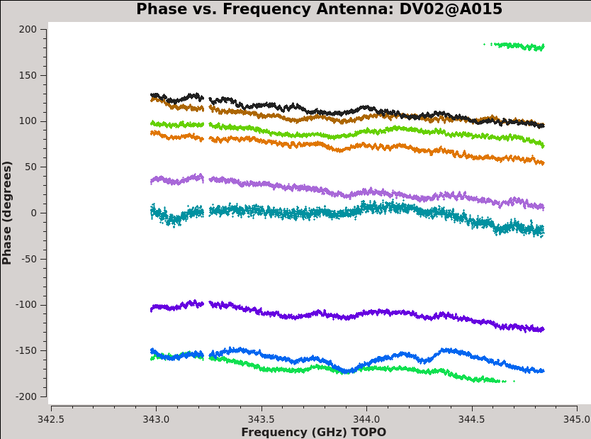
# In CASA
basename_all=["uid___A002_X1ff7b0_Xb","uid___A002_X207fe4_X3a","uid___A002_X207fe4_X3b9",
     "uid___A002_X2181fb_X49","uid___A002_X1ff7b0_X1c8","uid___A002_X207fe4_X1f7",
     "uid___A002_X207fe4_X4d7","uid___A002_X215db8_X18","uid___A002_X215db8_X1d5",
     "uid___A002_X215db8_X392"]

for asdm in basename_all:
    plotms(vis= asdm+'.wvrtsys.ms',
            xaxis='freq', yaxis='phase',
            selectdata=True, field='3c279', correlation='XX',
            avgtime='1e8', avgscan=T, antenna='*&*',
            coloraxis='baseline', iteraxis='antenna')
    dummy_string = raw_input("Plotting phase vs. frequency for "+asdm+". Hit <Enter> for next data set or cycle through antennas.")
Each plot shows phase as a function of frequency for all baselines with one antenna for 3c279. We plot only the 'XX' correlation, colorizing by baseline. With iteraxis set to antenna the green arrows at the bottom of plotms will cycle through antennas. By using avgscan and a large avgtime we average all scans and integrations.
The phase (and amplitude) also varies as a function of time, as we saw before. Here are the similar plots for phase vs. time (see Figure 14).
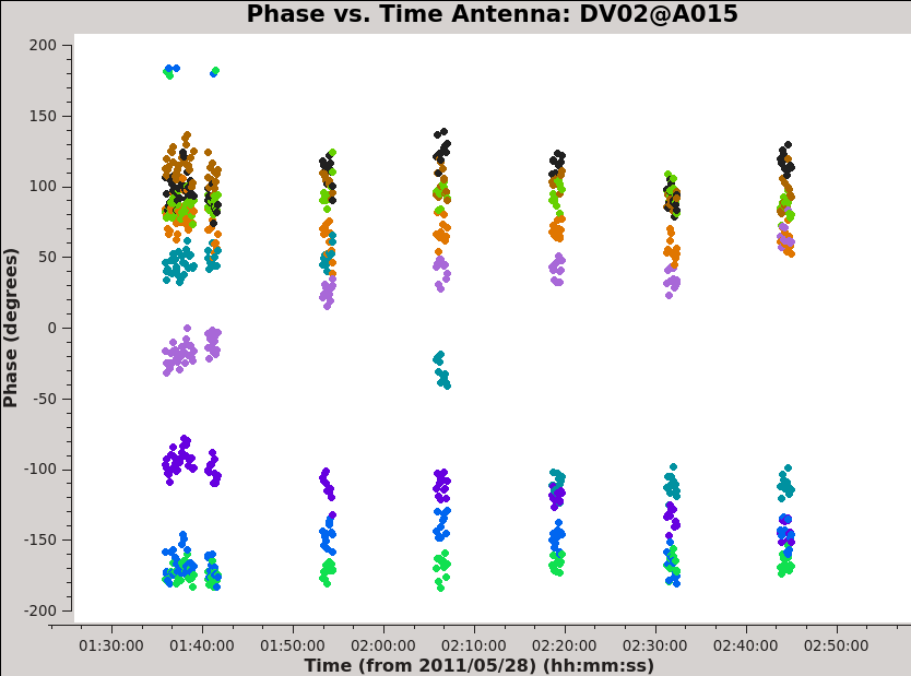
# In CASA
for asdm in basename_all:
    plotms(vis= asdm+'.wvrtsys.ms',
           xaxis='time', yaxis='phase',
           selectdata=True, field='3c279',
           spw='0:1200~1300', antenna='*&*',correlation='XX',
           avgchannel='1000',  avgscan=T,
           coloraxis='baseline', iteraxis='antenna')
    dummy_string = raw_input("Plotting phase vs. time for "+asdm+". Hit <Enter> for next data set or cycle through antennas.")
Figure 14 shows that the phase varies with time. We need to take this temporal variation into account when we solve for the frequency variations. Therefore we carry out the bandpass calibration in two steps. First, we use gaincal to solve for the variation of phase as a function of time for 3c279 on very short timescales. We set gaincal to derive a separate phase solution for each antenna every integration by setting solint to 'int'. We solve, averaging together only a small fraction of the total bandpass (channels 1100-1300) to avoid the effects of the phase vs. frequency behavior. We will then apply this solution to remove time-dependent behavior when we solve for the frequency response of the antennas with bandpass.
An integration is the smallest time quantum of observation in the data, usually a few seconds.
You can check the integration length for each scan in listobs.
#In CASA

for asdm in basename_all:
    print "Running a short solution interval phase calibration for "+asdm
    os.system('rm -rf '+asdm+'.bpphase.gcal')
    gaincal(vis = asdm+'.wvrtsys.ms',
               selectdata=T,field = '3c279',spw = '0:1100~1300',
               caltable = asdm+'.bpphase.gcal',
               solint = 'int',refant = 'DV11',calmode='p')
Now we use bandpass to solve for the frequency response of each antenna. To do this, we average all data in time by setting solint to 'inf' (that is, 'infinite'). We allow combination across scans and the different field IDs found for 3c279 by setting combine to "scan,field". We apply the phase vs. time calibration that we just derived on-the-fly using the parameter "gaintable".
for asdm in basename_all:
    print "Running a bandpass calibration for "+asdm
    os.system('rm -rf '+asdm+'.bandpass.bcal')
    bandpass(vis = asdm+'.wvrtsys.ms',
               field = '3c279',
               gaintable = asdm+'.bpphase.gcal',
               caltable = asdm+'.bandpass.bcal',
               bandtype='B',
               solint = 'inf',combine = 'scan,field', solnorm=T,refant = 'DV11',
               minblperant=3,minsnr=2,fillgaps=1)
in these calls:
- caltable specifies the output calibration table
- gaintable specifies any calibration tables to be applied "on the fly" to the data before solving.
- solint sets the time interval for which solutions are derived for each antenna.
- refant set the reference antenna, here DV11, which is defined to have zero correction by construction.
- calmode 'p' sets gaincal to calibrate the phase only, other options are 'a'mplitude or 'ap' - amplitude and phase.
- minblperant sets the minimum baselines required per antenna for a successful solution.
- minsnr sets the minimum signal-to-noise ratio required for a successful solution.
- bandtype here 'B' tells bandpass to solve for the phase and frequency response of each antenna in each channel, averaging data in time across the solution interval.
- fillgaps tells bandpass to interpolate across channel gaps 1 channel wide.
- solnorm tells bandpass to normalize the bandpass amplitude and phase corrections to have magnitude unity. The absolute scale of the calibration will come from our later gaincal solutions.
Do not worry about the message "Insufficient unflagged antennas" when running the bandpass task. This indicates that bandpass is failing on the flagged edge channels, which is expected.
It is now a good idea to plot both sets of solutions to look for irregularities, especially:
- discontinuities in the phase vs. time solution
- rapid wrapping of phase in either phase vs. time or bandpass solution
- large roll-off in the amplitude response near the band edge in the bandpass solution
- large scatter in any solution.
We loop through and using plotcal, again generating .png files of each calibration and splitting into two antenna groups for easier legibility. As the bandpass plots take a while you may want to go have a cup of coffee and inspect them using your favorite image viewer. Uncomment the raw_input line and switch the showgui parameter to True to see them in real time instead.
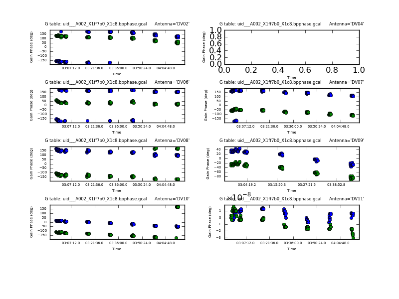
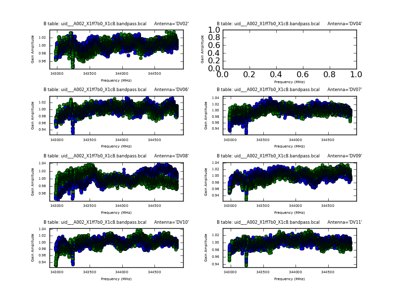
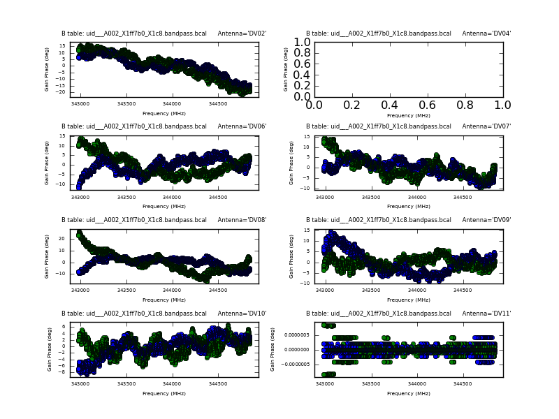
#In CASA

for asdm in basename_all:
    print "Plotting solutions for "+asdm
    plotcal(caltable = asdm+'.bpphase.gcal',
              xaxis = 'time', yaxis = 'phase', fontsize=6.0,
              iteration = 'antenna',
              showgui=False, subplot=421, figfile=asdm+'.bpphase.page1.png',
              antenna='0~7')
    # dummy_string = raw_input("Hit <Enter> to see next plot.")
    plotcal(caltable = asdm+'.bpphase.gcal',
              xaxis = 'time', yaxis = 'phase',
              iteration = 'antenna', fontsize=6.0,
              showgui=False, subplot=421, figfile=asdm+'.bpphase.page2.png',
              antenna='8~15')
    # dummy_string = raw_input("Hit <Enter> to see next plot.")
    plotcal(caltable = asdm+'.bandpass.bcal',
              xaxis = 'freq',yaxis = 'amp',
              antenna='0~7', iteration='antenna', fontsize=6.0,
              showgui=False, subplot=421, figfile=asdm+'.bcal_amp.page1.png')
    # dummy_string = raw_input("Hit <Enter> to see next plot.")
    plotcal(caltable = asdm+'.bandpass.bcal',
              xaxis = 'freq',yaxis = 'amp',
              antenna='8~15', iteration='antenna', fontsize=6.0,
              showgui=False, subplot=421, figfile=asdm+'.bcal_amp.page2.png')
    # dummy_string = raw_input("Hit <Enter> to see next plot.")
    plotcal(caltable = asdm+'.bandpass.bcal',
              xaxis = 'freq',yaxis = 'phase', iteration='antenna',
              antenna='0~7', subplot=421, figfile=asdm+'.bcal_phase.page1.png',
              showgui=False, fontsize=6.0)
    # dummy_string = raw_input("Hit <Enter> to see next plot.")
    plotcal(caltable = asdm+'.bandpass.bcal',
              xaxis = 'freq',yaxis = 'phase', iteration='antenna',
              antenna='8~15', subplot=421, figfile=asdm+'.bcal_phase.page2.png',
              showgui=False, fontsize=6.0)
    # dummy_string = raw_input("Hit <Enter> to see next plot.")
Gain (Phase and Amplitude) Calibration
The bandpass calibration will account for the phase and amplitude response of our antennas as a function of frequency. We now solve for the absolute flux scale of the data by referencing to Titan and then calibrate the phase and amplitude behavior of the antennas as a function of time.
Before using Titan to set the flux, there is an important systematic to account for. When we looked at the integrated spectra of our targets above, remember that Titan showed a whopping spectral line, in fact the same CO(3-2) line that we wish to observe in the Antennae. We will set the flux of Titan (and thus all of our data) by referencing to a model in casa that does not account for this line. Therefore we need to flag the part of the Titan observations contaminated by the line before we calibrate (you can see the affected channel range in Fig. 16). We run the following additional flagging step:
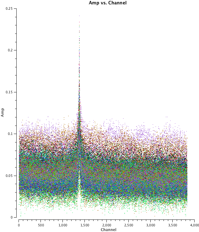
# in CASA
basename_all=["uid___A002_X1ff7b0_Xb","uid___A002_X207fe4_X3a","uid___A002_X207fe4_X3b9",
     "uid___A002_X2181fb_X49","uid___A002_X1ff7b0_X1c8","uid___A002_X207fe4_X1f7",
     "uid___A002_X207fe4_X4d7","uid___A002_X215db8_X18","uid___A002_X215db8_X1d5",
     "uid___A002_X215db8_X392"]

for asdm in basename_all:
    print "Flagging CO(3-2) in Titan for "+asdm
    flagdata(vis=asdm+'.wvrtsys.ms',flagbackup=F,
         field=['Titan'],
         spw=['0:1100~1700'])
    flagmanager(vis =asdm+'.wvrtsys.ms',mode = 'save',versionname = 'Calibration')
Next, we will use the setjy task to read the predicted complex visibilities for Titan into the MODEL column of each data set.
# in CASA
for asdm in basename_all:
    print "Reading model for Titan into "+asdm
    setjy(vis = asdm+'.wvrtsys.ms',field = 'Titan',
           standard = 'Butler-JPL-Horizons 2010')
setjy will output the flux of Titan to the CASA logger and it is worth recording this information. The flux of Titan at these frequencies is about 2.9 Jy. For example, for dataset uid___A002_X1ff7b0_Xb.wvrtsys.ms:
#2011-07-13 07:31:04 INFO setjy Titan spwid= 0 [I=2.847, Q=0, U=0, V=0] Jy
Next we'll run a short-solution interval gaincal to solve for phase variation on short timescales during observations of our two calibrators, with solint set to "int". By applying this on-the-fly, we can remove any decorrelation in the data due to phase scatter when we solve for the amplitude calibration. However, there is no benefit to using this short-timescale solution to calibrate the source because we only have information on the gain during calibrator visits (though see the Imaging portion of this guide). Instead we will solve for the gains to apply to the source using a longer solint in just a moment.
# in CASA

for asdm in basename_all:
    print "Carrying out short timescale phase solution for "+asdm
    os.system('rm -rf '+asdm+'.intphase.gcal')
    gaincal(vis=asdm+'.wvrtsys.ms',
                gaintable=asdm+'.bandpass.bcal',
                caltable=asdm+'.intphase.gcal',
                calmode='p',
                field='Titan,3c279',
                spw='0:40~3800',
                refant='DV11', solint='int',minsnr=2.0, minblperant=4)
Now we derive the longer timescale phase calibration table using solint set to "inf", but not allowing scan combination. This calibration has higher signal to noise due to combining more data, and for the purposes of correcting the source, it is just as precise as the short timescale solution.
# in CASA

for asdm in basename_all:
    print "Carrying out longer timescale phase solution for "+asdm
    os.system('rm -rf '+asdm+'.scanphase.gcal')
    gaincal(vis=asdm+'.wvrtsys.ms',
                gaintable=asdm+'.bandpass.bcal',
                caltable=asdm+'.scanphase.gcal',
                calmode='p',
                field='Titan,3c279',
                spw='0:40~3800',
                refant='DV11', solint='inf',minsnr=2.0,minblperant=4)
Now we apply the short-timescale phase solution and carry out a scan length (solint set to "inf") calibration of the data using calmode of 'a'.
# in CASA

for asdm in basename_all:
    print "Solving for longer (scan) interval amplitude solution for "+asdm
    os.system('rm -rf '+asdm+'.amp.cal')
    gaincal(vis = asdm+'.wvrtsys.ms',
               gaintable =[asdm+'.bandpass.bcal',asdm+'.intphase.gcal'],
               caltable = asdm+'.amp.cal',
               calmode='ap',
               field = 'Titan,3c279',
               spw='0:40~3800',
               refant = 'DV11',solint = 'inf', minblperant=4)
This "amp.cal" solution gives us the amplitude variations as a function of time, but they are not yet pinned to a realistic scale except in the case of Titan, where we have solved using the model input by setjy. We will set the flux of our secondary calibrator 3c279 with reference to Titan using fluxscale.
# in CASA

for asdm in basename_all:
    print "Scaling amplitude calibration to match Titan for "+asdm
    os.system('rm -rf '+asdm+'.flux.cal')
    fluxscale(vis = asdm+'.wvrtsys.ms',
                 caltable = asdm+'.amp.cal',
                 fluxtable = asdm+'.flux.cal',
                 reference = 'Titan',
                 transfer = '3c279')
This new correctly-scaled flux table ".flux.cal" replaces the previous ".amp.cal" table as the correct amplitude calibration table to apply to the data, i.e., the ".flux.cal" contains both the time variability of the amplitude solved for in ".amp.cal" and the correct flux scaling set with fluxscale.
Fluxscale will output the derived flux for 3c279 to the CASA logger. This information is worth noting. We find that the flux of 3c279 is 10.45 Jy, by averaging the fluxes obtained from the ten available datasets. This value agrees within 10% with the most recent 0.850 millimeter measurements from the SMA calibrator list [1] : (01 Jul 2011, SMA 9.75 ± 0.49).
Now we plot the final phase and amplitude calibration tables for each data set. A well-behaved calibration table will show smooth variations as a function of time. Sudden jumps or wild variations among the antenna amplitude gains should prompt further investigation and possibly additional flagging.
# in CASA

for asdm in basename_all:
    print "Plotting solutions for "+asdm
    plotcal(caltable = asdm+'.scanphase.gcal',
              xaxis = 'time', yaxis = 'phase',
              iteration = 'antenna', plotrange=[0,0,-180,180],
              showgui=False, subplot=421, figfile=asdm+'.scanphase.page1.png',
              antenna='0~7', fontsize=6.0)
    # dummy_string = raw_input("Hit <Enter> to see next plot.")
    plotcal(caltable = asdm+'.scanphase.gcal',
              xaxis = 'time', yaxis = 'phase',
              iteration = 'antenna', plotrange=[0,0,-180,180],
              showgui=False, subplot=421, figfile=asdm+'.scanphase.page2.png',
              antenna='8~15', fontsize=6.0)
    # dummy_string = raw_input("Hit <Enter> to see next plot.")
    plotcal(caltable = asdm+'.flux.cal',
              xaxis = 'time',yaxis = 'amp',
              plotrange = [0,0,0,0],
              antenna='0~7', iteration='antenna',
              showgui=False, subplot=421, figfile=asdm+'.flux.page1.png',
              fontsize=6.0)
    # dummy_string = raw_input("Hit <Enter> to see next plot.")
    plotcal(caltable = asdm+'.flux.cal',
              xaxis = 'time',yaxis = 'amp',
              plotrange = [0,0,0,0],
              antenna='8~15', iteration='antenna', fontsize=6.0,
              showgui=False, subplot=421, figfile=asdm+'.flux.page2.png')
    # dummy_string = raw_input("Hit <Enter> to see next plot.")
Apply the Calibrations and Inspect
Now we will use applycal to apply the bandpass, phase, and amplitude calibration tables that we generated in the previous sections to the data. We apply the solutions separately to the bandpass and secondary ("phase") calibrator 3c279, the flux calibrator Titan, and the target source. In most data sets, the bandpass and secondary calibrator will not be the same and this step would include one additional applycal.
#In CASA
basename_north=["uid___A002_X1ff7b0_Xb","uid___A002_X207fe4_X3a","uid___A002_X207fe4_X3b9","uid___A002_X2181fb_X49"]

for asdm in basename_north:
    print "Applying calibrations for "+asdm
    applycal(vis=asdm+'.wvrtsys.ms',field='3c279',
        gaintable=[asdm+'.bandpass.bcal',asdm+'.intphase.gcal',asdm+'.flux.cal'],
        interp=['nearest','nearest','nearest'],
        gainfield=['3c279','3c279','3c279'],flagbackup=F,calwt=T)
    applycal(vis=asdm+'.wvrtsys.ms',field='Titan',
        gaintable=[asdm+'.bandpass.bcal',asdm+'.intphase.gcal',asdm+'.flux.cal'],
        interp=['nearest','nearest','nearest'],
        gainfield=['3c279','Titan','Titan'],flagbackup=F,calwt=T)
    applycal(vis=asdm+'.wvrtsys.ms',field='NGC*',
        interp=['nearest','linear','linear'],
        gaintable=[asdm+'.bandpass.bcal',asdm+'.scanphase.gcal',asdm+'.flux.cal'],
        gainfield=['3c279','3c279','3c279'],flagbackup=F,calwt=T)

basename_south=["uid___A002_X1ff7b0_X1c8","uid___A002_X207fe4_X1f7","uid___A002_X207fe4_X4d7",
                           "uid___A002_X215db8_X18","uid___A002_X215db8_X1d5","uid___A002_X215db8_X392"]

for asdm in basename_south:
    print "Applying calibrations for "+asdm
    applycal(vis=asdm+'.wvrtsys.ms',field='3c279',
        gaintable=[asdm+'.bandpass.bcal',asdm+'.intphase.gcal',asdm+'.flux.cal'],
        interp=['nearest','nearest','nearest'],
        gainfield=['3c279','3c279','3c279'],flagbackup=F,calwt=T)
    applycal(vis=asdm+'.wvrtsys.ms',field='Titan',
        gaintable=[asdm+'.bandpass.bcal',asdm+'.intphase.gcal',asdm+'.flux.cal'],
        interp=['nearest','nearest','nearest'],
        gainfield=['3c279','Titan','Titan'],flagbackup=F,calwt=T)
    applycal(vis=asdm+'.wvrtsys.ms',field='Ant*',
        interp=['nearest','linear','linear'],
        gaintable=[asdm+'.bandpass.bcal',asdm+'.scanphase.gcal',asdm+'.flux.cal'],
        gainfield=['3c279','3c279','3c279'],flagbackup=F,calwt=T)
Here:
- vis and field specify the measurement set and field to calibrate.
- gaintable specifies the tables to apply to the data. There may be several tables applied all at once, here we apply the bandpass, phase, and flux calibrations.
- interp specifies the type of interpolation used to match calibration tables to the data. If there are several gaintables then interp may be either a single value (e.g., "linear" or "nearest") or a list of values with size equal to the list of gaintables. In the case where interp is a list, applycal will match each element to the corresponding gaintable (e.g., first gaintable with first interp parameter).
- gainfield specifies field from which to draw the calibration. As with interp, this can be a list of size matched to gaintable, so that the first element of gainfield will be the field used for the first table. For example, in the above commands the bandpass calibration (the first table) will always be applied from '3c279' (the first gainfield).
- calwt indicates that the weights, which were derived from the Tsys measurements, should also be calibrated. Note that calwt is True by default.
Once calibrations are applied, it is important to go back and inspect the calibrated data. New problematic antennas or baselines may be visible after calibration. Repeat the steps above, focusing on the CORRECTED data column. Bear in mind that for any point source calibrators we now expect to find phase scattering around zero and to find flat amplitudes as a function of u-v distance. Look for outliers and other signatures of problematic data. As a general rule, you will want to incorporate these data into your overall flagging script then rerun the whole calibration process, so that reduction is iterative. If the data only represent a minor problem, however, it may not be terribly harmful to flag them after the fact so that they do not interfere with imaging but trust that the calibrations are mostly unaffected.
As an example of this inspection, we cycle through the corrected amplitudes and phases of 3c279 as a function u-v distance, to check that the phases are close to zero and the amplitudes are constant.
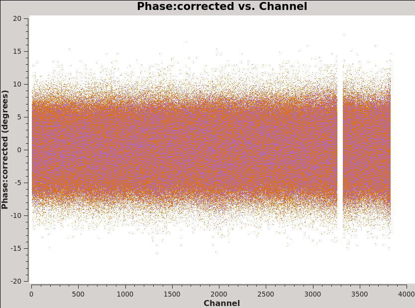
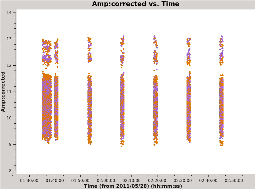
# In CASA

basename_all=["uid___A002_X1ff7b0_Xb","uid___A002_X207fe4_X3a","uid___A002_X207fe4_X3b9",
     "uid___A002_X2181fb_X49","uid___A002_X1ff7b0_X1c8","uid___A002_X207fe4_X1f7",
     "uid___A002_X207fe4_X4d7","uid___A002_X215db8_X18","uid___A002_X215db8_X1d5",
     "uid___A002_X215db8_X392"]

for asdm in basename_all:
    print "Examining calibrated data for "+asdm
    plotms(vis = asdm+'.wvrtsys.ms', xaxis='uvdist', yaxis='amp',
	ydatacolumn='corrected', field='3c279',
	averagedata=True, avgchannel='3840', avgtime='',
	avgscan=F, avgbaseline=F, coloraxis='corr')
    dummy_string = raw_input("Hit <Enter> for next plot.")
    plotms(vis = asdm+'.wvrtsys.ms', xaxis='time', yaxis='amp',
	ydatacolumn='corrected', field='3c279',
	averagedata=True, avgchannel='3840', avgtime='',
	avgscan=F, avgbaseline=F, coloraxis='corr')
    dummy_string = raw_input("Hit <Enter> for next plot.")
    plotms(vis = asdm+'.wvrtsys.ms', xaxis='uvdist', yaxis='phase',
	ydatacolumn='corrected', field='3c279',
	avgchannel='3840', avgscan=F, avgbaseline=F, coloraxis='corr')
    dummy_string = raw_input("Hit <Enter> for next plot.")
    plotms(vis = asdm+'.wvrtsys.ms', xaxis='time', yaxis='phase',
	ydatacolumn='corrected', field='3c279',
	avgchannel='3840', avgscan=F, avgbaseline=F, coloraxis='corr')
    dummy_string = raw_input("Hit <Enter> for next plot.")
In Fig. 17 and 18 we plot phase vs. channel and amp vs. time for 3c279 for the uid___A002_X1ff7b0_Xb dataset.
Finally we can use plotms to examine the corrected amplitude and phase of Antennae galaxies as a function of time and uv-distance (plots not shown):
# In CASA

for asdm in basename_north:
    print "Examining calibrated data for "+asdm
    plotms(vis = asdm+'.wvrtsys.ms', xaxis='uvdist', yaxis='amp',
	ydatacolumn='corrected', field='NGC*',
	averagedata=True, avgchannel='3840', avgtime='',
	avgscan=F, avgbaseline=F, coloraxis='corr')
    dummy_string = raw_input("Hit <Enter> for next plot.")
    plotms(vis = asdm+'.wvrtsys.ms', xaxis='time', yaxis='amp',
	ydatacolumn='corrected', field='NGC*',
	averagedata=True, avgchannel='3840', avgtime='',
	avgscan=F, avgbaseline=F, coloraxis='corr')
    dummy_string = raw_input("Hit <Enter> for next plot.")
    plotms(vis = asdm+'.wvrtsys.ms', xaxis='uvdist', yaxis='phase',
	ydatacolumn='corrected', field='NGC*',
	avgchannel='3840', avgscan=F, avgbaseline=F, coloraxis='corr')
    dummy_string = raw_input("Hit <Enter> for next plot.")
    plotms(vis = asdm+'.wvrtsys.ms', xaxis='time', yaxis='phase',
	ydatacolumn='corrected', field='NGC*',
	avgchannel='3840', avgscan=F, avgbaseline=F, coloraxis='corr')
    dummy_string = raw_input("Hit <Enter> for next plot.")

for asdm in basename_south:
    print "Examining calibrated data for "+asdm
    plotms(vis = asdm+'.wvrtsys.ms', xaxis='uvdist', yaxis='amp',
	ydatacolumn='corrected', field='Ant*',
	averagedata=True, avgchannel='3840', avgtime='',
	avgscan=F, avgbaseline=F, coloraxis='corr')
    dummy_string = raw_input("Hit <Enter> for next plot.")
    plotms(vis = asdm+'.wvrtsys.ms', xaxis='time', yaxis='amp',
	ydatacolumn='corrected', field='Ant*',
	averagedata=True, avgchannel='3840', avgtime='',
	avgscan=F, avgbaseline=F, coloraxis='corr')
    dummy_string = raw_input("Hit <Enter> for next plot.")
    plotms(vis = asdm+'.wvrtsys.ms', xaxis='uvdist', yaxis='phase',
	ydatacolumn='corrected', field='Ant*',
	avgchannel='3840', avgscan=F, avgbaseline=F, coloraxis='corr')
    dummy_string = raw_input("Hit <Enter> for next plot.")
    plotms(vis = asdm+'.wvrtsys.ms', xaxis='time', yaxis='phase',
	ydatacolumn='corrected', field='Ant*',
	avgchannel='3840', avgscan=F, avgbaseline=F, coloraxis='corr')
    dummy_string = raw_input("Hit <Enter> for next plot.")
Split and Concatenate Data for Northern and Southern Mosaics
The individual data sets are now calibrated. We can safely split out the calibrated data for our science target and drop the calibrators. As we do so, we will smooth the data in frequency, averaging together groups of 23 channels by setting width=23 in split. The new data will have a channel width corresponding to about ~10 km/s, very similar to the SMA data being verified. The factor of >20 drop in data volume will also make the imaging steps much more tractable.
#In CASA

basename_north=["uid___A002_X1ff7b0_Xb","uid___A002_X207fe4_X3a","uid___A002_X207fe4_X3b9","uid___A002_X2181fb_X49"]

basename_south=["uid___A002_X1ff7b0_X1c8","uid___A002_X207fe4_X1f7","uid___A002_X207fe4_X4d7",
                           "uid___A002_X215db8_X18","uid___A002_X215db8_X1d5","uid___A002_X215db8_X392"]

for asdm in basename_north:
    os.system('rm -rf '+asdm+'.cal.ms')
    split(vis = asdm+'.wvrtsys.ms',outputvis = asdm+'.cal.ms',
             field = 'NGC*',spw='0',width=23, keepflags=False)
    os.system('rm '+asdm+'.cal.listobs.txt')
    listobs(asdm+'.cal.ms',listfile=asdm+'.cal.listobs.txt')

for asdm in basename_south:
    os.system('rm -rf '+asdm+'.cal.ms')
    split(vis = asdm+'.wvrtsys.ms',outputvis = asdm+'.cal.ms',
             field = 'Ant*',spw='0',width=23, keepflags=False)
    os.system('rm '+asdm+'.cal.listobs.txt')
    listobs(asdm+'.cal.ms',listfile=asdm+'.cal.listobs.txt')
For convenience we concatenate all data for the Northern Mosaic into a single big MS and place all data for the Southern Mosaic into another file. To do this, we construct a list that holds the names of all the Southern Mosaic MS files and another that holds the name of all the Northern Mosaic MS files then feed these into the concat task.
Before we do this, we'll take a brief aside to remove Pointing information from the calibrated data. Normally, the pointing information would apply important corrections to be used while imaging the data. However, some aspects of this are still under development and the pointing information in these data interacts poorly with CASA. We will remove the pointing information using the CASA toolkit Table tool (tb). This kind of operation is dangerous and should not be a regular feature of your CASA reduction.
# In CASA

basename_all=["uid___A002_X1ff7b0_Xb","uid___A002_X207fe4_X3a","uid___A002_X207fe4_X3b9",
     "uid___A002_X2181fb_X49","uid___A002_X1ff7b0_X1c8","uid___A002_X207fe4_X1f7",
     "uid___A002_X207fe4_X4d7","uid___A002_X215db8_X18","uid___A002_X215db8_X1d5",
     "uid___A002_X215db8_X392"]

for asdm in basename_all:
    print "Manually removing pointing table from "+asdm+".cal.ms ... Please be careful!"
    tb.open(asdm+'.cal.ms/POINTING',nomodify=False)
    a = tb.rownumbers()
    tb.removerows(a)
    tb.close()
# In CASA

cal_south_vis = [vis+'.cal.ms' for vis in basename_south]
cal_north_vis = [vis+'.cal.ms' for vis in basename_north]

os.system('rm -rf Antennae_South.cal.ms')
concat(vis=cal_south_vis, concatvis='Antennae_South.cal.ms', timesort=T)

os.system('rm -rf Antennae_North.cal.ms')
concat(vis=cal_north_vis, concatvis='Antennae_North.cal.ms', timesort=T)
The syntax used to construct the 'cal_south_vis' variable loops over basename_south and makes a list after adding '.cal.ms' to each member. To see the list 'print cal_south_vis'.
Continue on to Imaging of the Science Target
Now you can continue on to the imaging guide.
Last checked on CASA Version 3.3.0.