Etime study: Difference between revisions
No edit summary |
No edit summary |
||
| (7 intermediate revisions by the same user not shown) | |||
| Line 1: | Line 1: | ||
A realistic simulation will have a short integration time (~3s-10s) to calculate visibilities at complete uv coverage and density. <font color="red">Real</font> observations with ALMA should not exceed ~10s integration (sample) times. | |||
However, corrupting with thermal noise is (currently - we're working on it) quite slow, and such a simulation can take hours to run. We suggest that you increase the integration time by up to an order of magnitude - if you have a long track with full ALMA, the uv coverage will still be quite realistic, and the simulation will run an order of magnitude faster. For early science simulations or snapshots with poorer uv coverage, the short integration time will be required (but for early science the speed won't be an issue since there are so many fewer baselines). | |||
Here is an example of the M51 simulation (8hr track) with 10, 15, 30, 120, and 240s integration times, and the correspondingly decreasing number of time samples in the Measurement Set: | Here is an example of the M51 simulation (8hr track) with 10, 15, 30, 120, and 240s integration times, and the correspondingly decreasing number of time samples in the Measurement Set: | ||
{| style="width: 100%; valign: top; background-color:#E0FFFF; border:1px solid #3366FF; " cellpadding=1 | {| style="width: 100%; valign: top; background-color:#E0FFFF; border:1px solid #3366FF; " cellpadding=1 | ||
| etime | |||
| uv | |||
| ch6 image | |||
|- | |- | ||
| | | 10s | ||
| (indistinguishable from 30s) | |||
| [[File:M51.10s.ch6.png|300px]] | |||
|- | |- | ||
| | | 15s | ||
| (indistinguishable from 30s) | |||
| [[File:M51.15s.ch6.png|300px]] | |||
|- | |||
| 30s | |||
| [[File:M51.30s.uv.png|300px]] | |||
| [[File:M51.30s.ch6.png|300px]] | |||
|- | |||
| 120s | |||
| [[File:M51.120s.uv.png|300px]] | |||
| [[File:M51.120s.ch6.png|300px]] | |||
|- | |||
| 240s | |||
| [[File:M51.240s.uv.png|300px]] | |||
| [[File:M51.240s.ch6.png|300px]] | |||
|- | |- | ||
|} | |} | ||
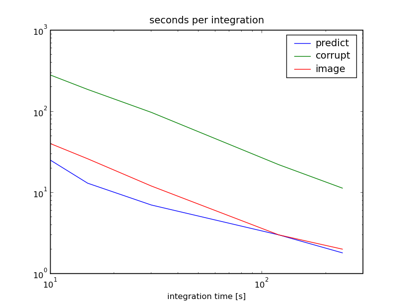
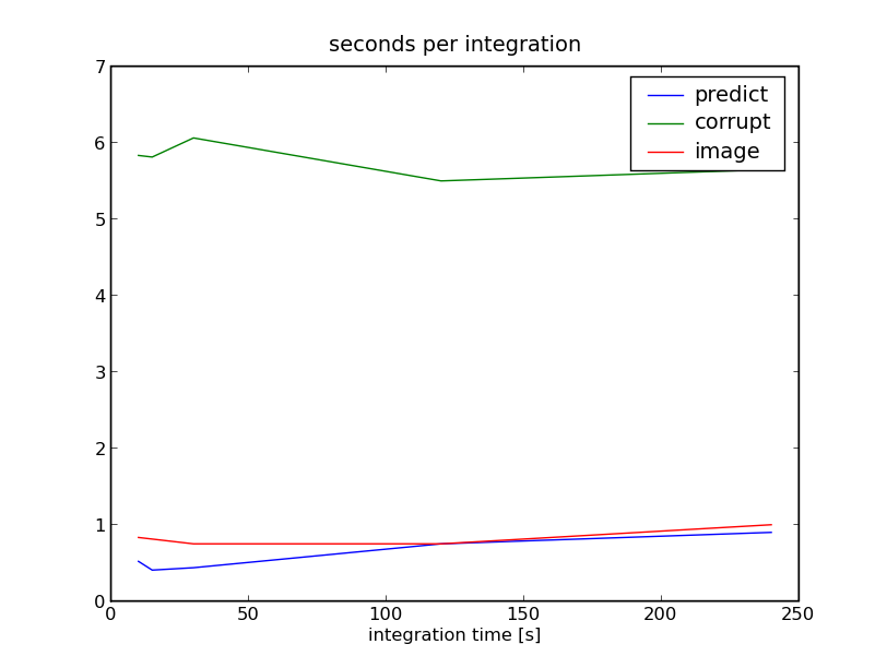
The uv coverage is slightly less filled at 240s integration, but the runtime is >20x faster: Plot of runtime as a function of integration time, and plot of runtime as a function of integration time divided by the number of samples (8hr/integration time). Each plot is split into the time required to predict visibilities, corrupt the data, and then re-image the corrupted visibilities: | |||
{| | |||
| [[File:M51.time.png|300px]] | |||
| [[File:M51.timeper.png|300px]] | |||
|- | |||
|} | |||
Naturally, what is of interest is if the images are quantitatively the same, and they are: This is the rms measured in several places: | |||
[[File:M51.rms.png|300px]] | |||
Latest revision as of 14:54, 9 June 2010
A realistic simulation will have a short integration time (~3s-10s) to calculate visibilities at complete uv coverage and density. Real observations with ALMA should not exceed ~10s integration (sample) times.
However, corrupting with thermal noise is (currently - we're working on it) quite slow, and such a simulation can take hours to run. We suggest that you increase the integration time by up to an order of magnitude - if you have a long track with full ALMA, the uv coverage will still be quite realistic, and the simulation will run an order of magnitude faster. For early science simulations or snapshots with poorer uv coverage, the short integration time will be required (but for early science the speed won't be an issue since there are so many fewer baselines).
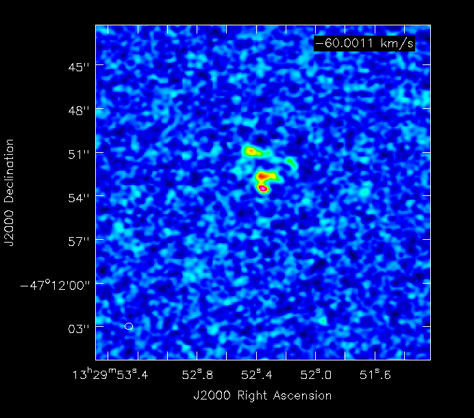
Here is an example of the M51 simulation (8hr track) with 10, 15, 30, 120, and 240s integration times, and the correspondingly decreasing number of time samples in the Measurement Set:
| etime | uv | ch6 image |
| 10s | (indistinguishable from 30s) | 
|
| 15s | (indistinguishable from 30s) | 
|
| 30s | 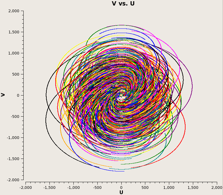
|

|
| 120s | 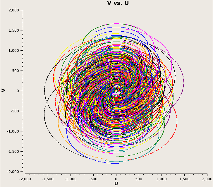
|
|
| 240s | 
|

|
The uv coverage is slightly less filled at 240s integration, but the runtime is >20x faster: Plot of runtime as a function of integration time, and plot of runtime as a function of integration time divided by the number of samples (8hr/integration time). Each plot is split into the time required to predict visibilities, corrupt the data, and then re-image the corrupted visibilities:
|
|
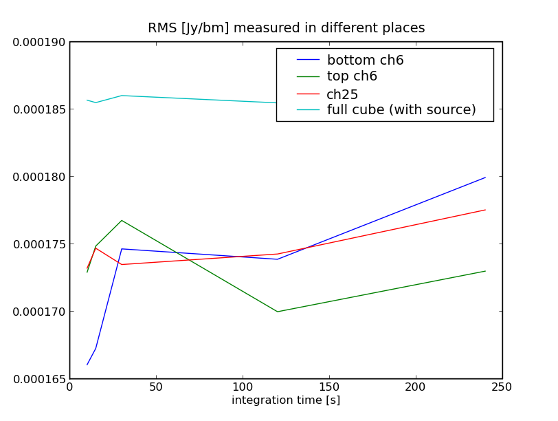
Naturally, what is of interest is if the images are quantitatively the same, and they are: This is the rms measured in several places:
