3C286 Band6Pol Imaging for CASA 6.6.1: Difference between revisions
mNo edit summary |
|||
| (127 intermediate revisions by the same user not shown) | |||
| Line 3: | Line 3: | ||
==Overview== | ==Overview== | ||
This portion of the '''[[3C286 Polarization]]''' CASA Guide will cover the imaging of the | This portion of the '''[[3C286 Polarization]]''' CASA Guide will cover the imaging of the total intensity and polarized emission. | ||
total | |||
This guide picks up where the '''[[3C286 Band6Pol Calibration | Calibration]]''' section left off: right after running the CASA task {{split_6.6.1}} to split off the science target from the rest of the measurement set following calibration. If you completed the Calibration section of the guide, then you can continue where you left off, with ''3c286_Band6.pol.cal.ms''. | This guide picks up where the '''[[3C286 Band6Pol Calibration | Calibration]]''' section left off: right after running the CASA task {{split_6.6.1}} to split off the science target from the rest of the measurement set following calibration. If you completed the Calibration section of the guide, then you can continue where you left off, with ''3c286_Band6.pol.cal.ms''. | ||
| Line 12: | Line 11: | ||
Once the download has finished, unpack the file: | Once the download has finished, unpack the file: | ||
<source lang="bash"> | <source lang="bash"> | ||
# In a bash terminal outside CASA | |||
# In a terminal outside CASA | |||
tar -xvzf 3C286_Band6_CalibratedData.tgz | tar -xvzf 3C286_Band6_CalibratedData.tgz | ||
</source> | </source> | ||
<!-- cd 3C286_Band6_CalibratedData --> | |||
After that, you should have ''3c286_Band6.pol.cal.ms'' in your working directory. | After that, you should have ''3c286_Band6.pol.cal.ms'' in your working directory. | ||
{{CARTA_6.6.1}} | {{CARTA_6.6.1}} | ||
==Full polarization imaging of the target== | ==Full polarization imaging of the target== | ||
| Line 35: | Line 29: | ||
vis='3c286_Band6.pol.cal.ms' | vis='3c286_Band6.pol.cal.ms' | ||
</source> | </source> | ||
[[File:Target_uvplot_5.4.png|300px|thumb|right|'''Fig 1:''' Amplitude vs. uv-distance of 3c286. The source seems to be slightly resolved.]] | |||
Before starting the cleaning, it makes sense to check if the emission is resolved or not by plotting amplitude as a function of uv-distance. | Before starting the cleaning, it makes sense to check if the emission is resolved or not by plotting amplitude as a function of uv-distance. | ||
| Line 42: | Line 38: | ||
# In CASA | # In CASA | ||
plotms(vis, spw='', xaxis='uvwave', yaxis='amp', correlation='XX,YY', | plotms(vis, spw='', xaxis='uvwave', yaxis='amp', correlation='XX,YY', | ||
avgtime='1e8', avgchannel='1000', coloraxis='baseline' | avgtime='1e8', avgchannel='1000', coloraxis='baseline') | ||
</source> | </source> | ||
This plot also helps us defining the cellsize needed for the task clean. | This plot also helps us defining the cellsize needed for the task clean. | ||
From the plot we see that the longest baseline is 500 kilo wavelength. This means that the maximum resolution can be | * From the plot we see that the longest baseline is 500 kilo wavelength. This means that the maximum resolution can be approximately 1/500000*206265 arcsec = 0.4 arcsec. We will use a ''cellsize=0.1'', to oversample the beam sufficiently. | ||
approximately 1/500000*206265 arcsec = 0.4 arcsec. | * The FWHM of the primary beam of ALMA in Band 6 is about 25 arcsec, and we want to image out to at least that extent, so we will use ''imsize=250''. | ||
We will use a | * Since 3c286 is (nearly) a point source, we expect few clean components to be added to the model. To avoid over cleaning, set ''cycleniter'' to a small number like 10. | ||
[[File:3c286.StokesIQUV_interactive_tclean.png|300px|thumb|right|'''Fig 2:''' Check "All Polarizations" and then draw a tight mask around the source in the I plane.]] | |||
<source lang="python"> | <source lang="python"> | ||
# In CASA | # In CASA | ||
os.system('rm -rf 3c286.StokesIQUV*') | |||
os.system('rm -rf 3c286. | |||
tclean(vis, | tclean(vis, | ||
imagename = '3c286.StokesIQUV', | |||
cell = ['0.1arcsec'], | |||
imsize = [250,250], | |||
deconvolver = 'clarkstokes', | |||
stokes = 'IQUV', | |||
interactive = True, | |||
weighting = 'briggs', | |||
robust = 0.5, | |||
niter = 500, | |||
pbcor = True, | |||
cycleniter = 10) | |||
</source> | </source> | ||
Specifying | Specifying ''interactive=True'', the {{tclean_6.6.1}} task brings up a viewer to show the residual clean image, where clean masks can be defined. | ||
* Draw a tight mask around the central source, excluding the surrounding negative regions. See Figure 2. Carefully adjust the mask in each polarization plane as needed between each major cycle. | |||
When the residuals are noise-like, the cleaning process can be finished by clicking the red X symbol. | |||
Please note that the cleaning will not start without any active mask (to activate a mask you need to double click inside the region). | Please note that the cleaning will not start without any active mask (to activate a mask you need to double click inside the region). | ||
See [ | See [[First_Look_at_Imaging#First_Look_at_TCLEAN]] for further details on the interactive use of {{tclean_6.6.1}}. | ||
Finally, note that we delete any previous versions of the output images before proceeding with the clean command. This is important, because if images with the supplied root name already exist, CASA will clean those further instead of producing new output images. | Finally, note that we delete any previous versions of the output images before proceeding with the clean command. This is important, because if images with the supplied root name already exist, CASA will clean those further instead of producing new output images. | ||
After | After about the 5th major cycle (90 iterations, 410 remaining), the residuals are already noise-like, so you can stop the cleaning. | ||
To view your newly cleaned image, start CARTA. If using NRAO machines, you can open a new terminal tab, cd to the working directory, then type: | To view your newly cleaned image, start CARTA. If using NRAO machines, you can open a new terminal tab, cd to the working directory, then type: | ||
| Line 85: | Line 83: | ||
</source> | </source> | ||
Copy the output URL into a browser to view your CARTA session. Select and load < | Copy the output URL into a browser to view your CARTA session. Select and load:<br> ''3c286.StokesIQUV.image'' | ||
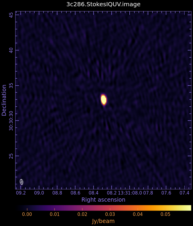
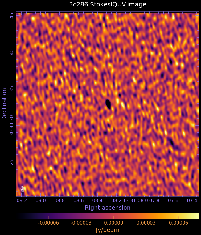
<gallery widths=250px heights=200px perrow=4 mode="packed" caption="Fig. 3: Full Polarization Image of 3c286. Scales are NOT matched."> | |||
File:3C286.StokesIQUV.image.I_6.6.1.png|Stokes I (total intensity) | |||
File:3C286.StokesIQUV.image.Q_6.6.1.png|Stokes Q (linear polarization) | |||
File:3C286.StokesIQUV.image.U_6.6.1.png|Stokes U (linear polarization) | |||
File:3C286.StokesIQUV.image.V_6.6.1.png|Stokes V (circular polarization) | |||
</gallery> | |||
We can check the restoring beam by opening the File Header tool and clicking the File Information tab:<br>0.76326" X 0.402745", 8.34021 deg | |||
Now draw a box in CARTA on the I plane away from the source and use the Statistics widget to determine the rms and max. Alternatively, use {{imstat_6.6.1}} as follows: | |||
<source lang="python"> | <source lang="python"> | ||
# In CASA | # In CASA | ||
calstat=imstat(imagename='3c286. | calstat = imstat(imagename='3c286.StokesIQUV.image', stokes='I', box='45,45,95,95') | ||
rms=(calstat['rms'][0]) | rms = (calstat['rms'][0]) | ||
calstat = imstat(imagename='3c286.StokesIQUV.image', stokes='I') | |||
peak = (calstat['max'][0]) | |||
print('>> rms in continuum image: '+str(rms)) | print('>> rms in continuum image: '+str(rms)) | ||
print('>> Peak in continuum image: '+str(peak)) | print('>> Peak in continuum image: '+str(peak)) | ||
print('>> Dynamic range in continuum image: '+str(peak/rms)) | print('>> Dynamic range in continuum image: '+str(peak/rms)) | ||
</source> | </source> | ||
<pre style="background-color: #fffacd; white-space: pre; overflow-x: auto;"> | |||
>> rms in continuum image: 0.001051827310962827 | |||
>> Peak in continuum image: 0.2975700795650482 | |||
>> Dynamic range in continuum image: 282.90773253706163 | |||
</pre> | |||
The rms of this image is ~1.05 mJy, the peak flux density is ~298 mJy, and the dynamic range (ratio of peak/rms) is ~283. | |||
== Self-calibration == | |||
The quality of the image can be improved by applying self-calibration to the uv data. See [[AntennaeBand7_Imaging]] for details on this technique. | |||
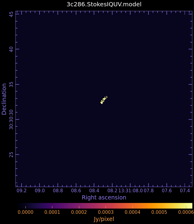
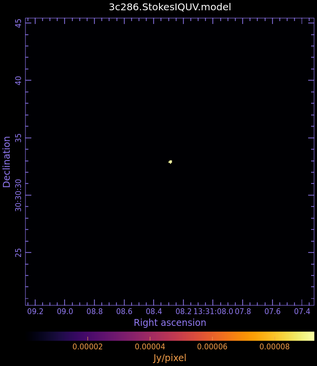
First, examine the model image we just created in CARTA:<br>''3c286.StokesIQUV.model'' | |||
<gallery widths=250px heights=200px perrow=4 mode="packed" caption="Fig. 4: Full Polarization Model Image of 3c286"> | |||
File:3C286.StokesIQUV.model.I_6.6.1.png|Stokes I | |||
File:3C286.StokesIQUV.model.Q_6.6.1.png|Stokes Q | |||
File:3C286.StokesIQUV.model.U_6.6.1.png|Stokes U | |||
File:3C286.StokesIQUV.model.V_6.6.1.png|Stokes V | |||
</gallery> | |||
For self-cal, it is generally better to do a shallow initial clean than a deep clean. If your model shows too much structure, you may want to redo the previous section with a shallower clean before proceeding. | |||
<div style="background-color: #E0FFFF; padding: 10px; font-family: 'Consolas', monospace;> | |||
For telescopes with linear feeds such as ALMA, I and Q are determined by parallel-hand correlations XX and YY, while U and V are determined by cross-hand correlations XY and YX. Therefore, calibrations in I also affect Q. To account for this, if there is emission in Q, then Q must have a reliable model before proceeding with the self-calibration of I. A low signal in Q may result in too poor of a model. For reference, see [https://science.nrao.edu/science/meetings/2018/16th-synthesis-imaging-workshop/talks/Schinzel_Polarization.pdf this 2018 SISS Lecture, slide 13]. | |||
</div> | |||
=== Prep === | |||
To proceed with self-calibration, first use {{tclean_6.6.1}} to read the model image and write model visibilities it into the MODEL column of the MS. | |||
'''The model image must be closed in CARTA before being read by tclean.''' | |||
<source lang="python"> | <source lang="python"> | ||
# In CASA | # In CASA | ||
tclean(vis, | |||
imagename = '3c286.StokesIQUV', | |||
cell = ['0.1arcsec'], | |||
imsize = [250,250], | |||
deconvolver = 'clarkstokes', | |||
stokes = 'IQUV', | |||
interactive = True, | |||
weighting = 'briggs', | |||
robust = 0.5, | |||
niter = 0, | |||
calcpsf = False, | |||
calcres = False, | |||
restoration = False, | |||
pbcor = True, | |||
savemodel = 'modelcolumn') | |||
</source> | </source> | ||
By default, savemodel = 'none', and the MS is opened in read-only mode. Ctrl+C can then be safely used to terminate tclean as needed. With savemodel = 'modelcolumn' (or 'virtual'), the MS will be written to, and using Ctrl+C may corrupt the MS. For the stand-alone step of reading an existing model image and writing model visibilities into the MS, choose niter = 0, calcpsf = False, calcres = False, restoration = False, and savemodel = 'modelcolumn'. | |||
Each round of self-calibration will follow the steps: | |||
# {{gaincal_6.6.1}}: create a self-calibration gain table | |||
# {{plotms_6.6.1}}: examine the table | |||
# {{applycal_6.6.1}}: apply the table | |||
# {{tclean_6.6.1}}: make a new image | |||
# {{imstat_6.6.1}}: determine image statistics | |||
Start with a long solution interval near the length of a target scan, and decrease with each round from there. | |||
=== | === Round 1 === | ||
[[Image:3c286_IQUV.G1p.png|500px|thumb|right|'''Fig 5:''' Phase-only self-calibration table with solint='300s'.]] | |||
Now create a self-calibration gain table with {{gaincal_6.6.1}}: | |||
<source lang="python"> | <source lang="python"> | ||
| Line 124: | Line 180: | ||
os.system('rm -rf 3c286_IQUV.G1p') | os.system('rm -rf 3c286_IQUV.G1p') | ||
gaincal(vis, | gaincal(vis, | ||
caltable='3c286_IQUV.G1p', | caltable = '3c286_IQUV.G1p', | ||
solint='300s', | solint = '300s', | ||
refantmode='strict', | refantmode = 'strict', | ||
refant='DV23',minblperant=4, | refant = 'DV23', | ||
calmode='p',minsnr=4) | minblperant = 4, | ||
calmode = 'p', | |||
minsnr = 4) | |||
</source> | </source> | ||
The critical parameters in this setup are | The critical parameters in this setup are ''solint''' and '''calmode''. | ||
We will force the reference antenna to remain constant with the | We will force the reference antenna to remain constant with the ''refantmode='strict'.'' | ||
We want to calculate phase solutions only so we use | We want to calculate phase solutions only so we use ''calmode=p'' and we start using ''solint=300s'', which averages in time close to the target scan length. | ||
It is usually best to start with a large solint and then go down to the integration time if the S/N of the data permits. | It is usually best to start with a large solint and then go down to the integration time if the S/N of the data permits. | ||
To check the quality of the solutions we obtained, we plot the gains for each antenna, as function of time: | To check the quality of the solutions we obtained, we plot the gains for each antenna, as function of time: | ||
| Line 141: | Line 198: | ||
<source lang="python"> | <source lang="python"> | ||
# In CASA | # In CASA | ||
plotms(vis='3c286_IQUV.G1p',xaxis='time',yaxis='phase',iteraxis='antenna', | plotms(vis='3c286_IQUV.G1p', xaxis='time', yaxis='phase', coloraxis='spw', iteraxis='antenna', gridrows=3, gridcols=2) | ||
</source> | </source> | ||
Now we apply those solutions to the uv data: | Now we apply those solutions to the uv data: | ||
| Line 149: | Line 205: | ||
<source lang="python"> | <source lang="python"> | ||
# In CASA | # In CASA | ||
applycal(vis, gaintable='3c286_IQUV.G1p') | |||
</source> | |||
<!-- | |||
Make a copy to match the self-cal image name we will create below. This is technically only necessary if you don't specify the mask name in {{tclean_6.6.1}}, in which case an existing mask in your working directory that matches the image name will be automatically applied. If you downloaded the calibrated data, you already have this mask file named ''3c286.StokesIQUV.mask''. | |||
To rename the file: | |||
<source lang="python"> | |||
# In CASA | |||
os.system('cp -r 3c286.StokesIQUV.mask 3c286.StokesIQUV.selfcal1.mask') | |||
</source> | </source> | ||
--> | |||
<!-- | |||
The mask you drew for the initial clean has been saved in your working directory as a file ''3c286.StokesIQUV.mask''. We will start with this same mask while cleaning our next image: | |||
--> | |||
Make a new image: | |||
<source lang="python"> | <source lang="python"> | ||
# In CASA | # In CASA | ||
os.system('rm -rf 3c286.StokesIQUV.selfcal1*') | |||
tclean(vis, | |||
imagename = '3c286.StokesIQUV.selfcal1', | |||
cell = ['0.1arcsec'], | |||
imsize = [250,250], | |||
deconvolver = 'clarkstokes', | |||
stokes = 'IQUV', | |||
interactive = True, | |||
weighting = 'briggs', | |||
robust = 0.5, | |||
pbcor = True, | |||
niter = 1000, | |||
cycleniter = 10, | |||
savemodel = 'modelcolumn') | |||
</source> | |||
Examine the image in CARTA (Fig 8) and determine new image statistics with {{imstat_6.6.1}}: | |||
calstat=imstat(imagename='3c286. | <source lang="python"> | ||
rms=(calstat['rms'][0]) | # In CASA | ||
calstat = imstat(imagename='3c286.StokesIQUV.selfcal1.image', stokes='I', box='45,45,95,95') | |||
rms = (calstat['rms'][0]) | |||
calstat = imstat(imagename='3c286.StokesIQUV.selfcal1.image', stokes='I') | |||
peak = (calstat['max'][0]) | |||
print('>> rms in continuum image: '+str(rms)) | print('>> rms in continuum image: '+str(rms)) | ||
print('>> Peak in continuum image: '+str(peak)) | print('>> Peak in continuum image: '+str(peak)) | ||
print('>> Dynamic range in continuum image: '+str(peak/rms)) | print('>> Dynamic range in continuum image: '+str(peak/rms)) | ||
</source> | |||
<pre style="background-color: #fffacd; white-space: pre; overflow-x: auto;"> | |||
>> rms in continuum image: 0.0002559800965899336 | |||
>> Peak in continuum image: 0.32107236981391907 | |||
>> Dynamic range in continuum image: 1254.2864624676654 | |||
</pre> | |||
The rms of this new image is ~0.256 mJy/beam, significantly lower than the value measured in the first image (1.05 mJy/beam). | |||
=== Round 2 === | |||
[[Image:3c286_IQUV.G2p.png|500px|thumb|right|'''Fig 6:''' Phase-only self-calibration table with solint='30s'.]] | |||
We run a second self-calibration, decreasing the solint to 30 sec, apply it to the data, and image it again: | |||
We run a second self-calibration, decreasing to 30 sec | |||
<source lang="python"> | <source lang="python"> | ||
| Line 193: | Line 271: | ||
os.system('rm -rf 3c286_IQUV.G2p') | os.system('rm -rf 3c286_IQUV.G2p') | ||
gaincal(vis, | gaincal(vis, | ||
caltable='3c286_IQUV.G2p', | caltable = '3c286_IQUV.G2p', | ||
solint='30s',refantmode='strict', | solint = '30s', | ||
refant='DV23',minblperant=4, | refantmode = 'strict', | ||
calmode='p',minsnr=4) | refant = 'DV23', | ||
minblperant = 4, | |||
calmode = 'p', | |||
minsnr = 4) | |||
</source> | |||
plotms(vis='3c286_IQUV.G2p',xaxis='time',yaxis='phase',iteraxis='antenna', | <source lang="python"> | ||
# In CASA | |||
plotms(vis='3c286_IQUV.G2p', xaxis='time', yaxis='phase', coloraxis='spw', iteraxis='antenna', gridrows=3, gridcols=2) | |||
</source> | |||
applycal(vis, | <source lang="python"> | ||
# In CASA | |||
applycal(vis, gaintable='3c286_IQUV.G2p') | |||
</source> | |||
os.system('rm -rf 3c286. | <source lang="python"> | ||
# In CASA | |||
os.system('rm -rf 3c286.StokesIQUV.selfcal2*') | |||
tclean(vis, | tclean(vis, | ||
imagename = '3c286.StokesIQUV.selfcal2', | |||
cell = ['0.1arcsec'], | |||
imsize = [250,250], | |||
deconvolver = 'clarkstokes', | |||
stokes = 'IQUV', | |||
interactive = True, | |||
weighting = 'briggs', | |||
robust = 0.5, | |||
pbcor = True, | |||
niter = 1000, | |||
cycleniter = 10, | |||
savemodel = 'modelcolumn') | |||
</source> | </source> | ||
<!-- | |||
You can notice when the first residual image appears that some residual central emission is evident. Continue the cleaning, by using the green continue button, until the residual image appears as much as possible noise like. | You can notice when the first residual image appears that some residual central emission is evident. Continue the cleaning, by using the green continue button, until the residual image appears as much as possible noise like. | ||
In this example we stop the clean after 2 cycles | In this example we stop the clean after 2 cycles. Examine the image in CARTA (Fig 8) and check the image statistics. | ||
--> | |||
<source lang="python"> | <source lang="python"> | ||
# In CASA | # In CASA | ||
calstat=imstat(imagename='3c286. | calstat = imstat(imagename='3c286.StokesIQUV.selfcal2.image', stokes='I', box='45,45,95,95') | ||
rms=(calstat['rms'][0]) | rms = (calstat['rms'][0]) | ||
calstat = imstat(imagename='3c286.StokesIQUV.selfcal2.image', stokes='I') | |||
peak = (calstat['max'][0]) | |||
print('>> rms in continuum image: '+str(rms)) | print('>> rms in continuum image: '+str(rms)) | ||
print('>> Peak in continuum image: '+str(peak)) | print('>> Peak in continuum image: '+str(peak)) | ||
print('>> Dynamic range in continuum image: '+str(peak/rms)) | print('>> Dynamic range in continuum image: '+str(peak/rms)) | ||
</source> | </source> | ||
<pre style="background-color: #fffacd; white-space: pre; overflow-x: auto;"> | |||
>> rms in continuum image: 0.0002521665039442129 | |||
>> Peak in continuum image: 0.3348853290081024 | |||
>> Dynamic range in continuum image: 1328.032564873047 | |||
</pre> | |||
The rms level in this new image is ~0.252 mJy/beam. This is only slightly less than than the previous round, so we will not reduce the solint further. | |||
=== Round 3 === | |||
solving for both amplitude and phase. | |||
[[Image:3c286_IQUV.Gap.png|500px|thumb|right|'''Fig 7:''' Amp and Phase self-calibration table with solint='30s'. Here we show amplitude.]] | |||
[[Image:3c286_IQUV_selfcal_comparison.png|400px|thumb|right|'''Fig 8:''' Stokes I image from before selfcal and after each round of selfcal for comparison. Raster scaling is matched.]] | |||
This level can be improved by a last run of self-calibration, this time solving for both amplitude and phase. | |||
<source lang="python"> | <source lang="python"> | ||
| Line 243: | Line 342: | ||
os.system('rm -rf 3c286_IQUV.Gap') | os.system('rm -rf 3c286_IQUV.Gap') | ||
gaincal(vis, | gaincal(vis, | ||
caltable='3c286_IQUV.Gap', | caltable = '3c286_IQUV.Gap', | ||
solint='30s', | gaintable = '3c286_IQUV.G2p', | ||
refant='DV23',minblperant=4 | solint = '30s', | ||
calmode='ap',minsnr=4) | refantmode = 'strict', | ||
refant = 'DV23', | |||
minblperant = 4, | |||
calmode = 'ap', | |||
minsnr = 4) | |||
</source> | |||
plotms(vis='3c286_IQUV.Gap',xaxis='time',yaxis=' | <source lang="python"> | ||
# In CASA | |||
plotms(vis='3c286_IQUV.Gap', xaxis='time', yaxis='phase', coloraxis='spw', iteraxis='antenna', gridrows=3, gridcols=2) | |||
plotms(vis='3c286_IQUV.Gap', xaxis='time', yaxis='amp', coloraxis='spw', iteraxis='antenna', gridrows=3, gridcols=2) | |||
</source> | |||
applycal(vis, | <source lang="python"> | ||
# In CASA | |||
applycal(vis, gaintable=['3c286_IQUV.G2p','3c286_IQUV.Gap']) | |||
</source> | |||
os.system('rm -rf 3c286. | <source lang="python"> | ||
# In CASA | |||
os.system('rm -rf 3c286.StokesIQUV.selfcal.ap*') | |||
tclean(vis, | tclean(vis, | ||
imagename = '3c286.StokesIQUV.selfcal.ap', | |||
cell = ['0.1arcsec'], | |||
imsize = [250,250], | |||
deconvolver = 'clarkstokes', | |||
stokes = 'IQUV', | |||
interactive = True, | |||
weighting = 'briggs', | |||
robust = 0.5, | |||
pbcor = True, | |||
niter = 1000, | |||
cycleniter = 10) | |||
</source> | </source> | ||
This time the first residual map shows a new bright extended component which was completely hidden by the noise in the previous images. We add a clean box around it and proceed with the clean. After 1000 cycles we stop and check the statistics | This time the first residual map shows a new bright extended component which was completely hidden by the noise in the previous images. We add a clean box around it and proceed with the clean. After 1000 cycles we stop. Examine the image in CARTA (Fig 8) and check the statistics: | ||
<source lang="python"> | <source lang="python"> | ||
# In CASA | # In CASA | ||
calstat=imstat(imagename='3c286. | calstat = imstat(imagename='3c286.StokesIQUV.selfcal.ap.image', stokes='I', box='45,45,95,95') | ||
rms=(calstat['rms'][0]) | rms = (calstat['rms'][0]) | ||
calstat = imstat(imagename='3c286.StokesIQUV.selfcal.ap.image', stokes='I') | |||
peak = (calstat['max'][0]) | |||
print('>> rms in continuum image: '+str(rms)) | print('>> rms in continuum image: '+str(rms)) | ||
print('>> Peak in continuum image: '+str(peak)) | print('>> Peak in continuum image: '+str(peak)) | ||
print('>> Dynamic range in continuum image: '+str(peak/rms)) | print('>> Dynamic range in continuum image: '+str(peak/rms)) | ||
</source> | </source> | ||
The rms is 0. | <pre style="background-color: #fffacd; white-space: pre; overflow-x: auto;"> | ||
>> rms in continuum image: 0.0001295028028448405 | |||
>> Peak in continuum image: 0.33380603790283203 | |||
>> Dynamic range in continuum image: 2577.597013886801 | |||
</pre> | |||
<!-- | |||
for calwt=False: | |||
>> rms in continuum image: 0.00013770987582083284 | |||
>> Peak in continuum image: 0.33382830023765564 | |||
>> Dynamic range in continuum image: 2424.1420468055776 | |||
--> | |||
The rms is 0.13 mJy, another significant decrease. We consider this result satisfying and stop the self-calibration. | |||
<!-- | |||
=== Summary === | |||
Below is a table to help summarize our process. D indicates data in the Data column, which doesn't change. M0, M1, and M2 are the incrementally improved models which are transformed into uv data and stored in the Model column. When calibration tables are applied to D, the result is saved in the Corrected column. | |||
{| class="wikitable" style="text-align:center;" | |||
| step | |||
! Data | |||
! Corrected | |||
! Model | |||
| description | |||
|- | |||
| No Selfcal | |||
| D | |||
| | |||
| | |||
| style="text-align:left;" | - make an initial image from D | |||
|- | |||
| Selfcal prep | |||
| D | |||
| | |||
| M0 | |||
| style="text-align:left;" | - save the initial model image M0 into the MS Model column | |||
|- | |||
| Round 1 | |||
| D | |||
| D*G1p | |||
| M1 | |||
| style="text-align:left;" | - solve for phase corrections G1p with long solint, using D and M0<br>- apply G1p and save result to Corrected<br>- create a new image from Corrected<br>- save new model image M1 to Model | |||
|- | |||
| Round 2 | |||
| D | |||
| D*G2p | |||
| M2 | |||
| style="text-align:left;" | - solve for phase corrections G2p with shorter solint, using D and M1<br>- apply G2p and save result to Corrected<br>- create a new image from Corrected<br>- save new model image M2 to Model | |||
|- | |||
| Round 3 | |||
| D | |||
| D*G2p*Gap | |||
| M2 | |||
| style="text-align:left;" | - solve for phase AND amp corrections Gap using D and M2 while applying G2p on-the-fly<br>- apply G2p AND Gap and save result to Corrected<br>- create a new image from Corrected | |||
|} | |||
<br clear='all'> | |||
--> | |||
== Stokes images == | |||
We can extract the Stokes Q, U, and V images from the | We can extract the Stokes I, Q, U, and V images from the self-calibrated image, using the task {{immath_6.6.1}}: | ||
<source lang="python"> | <source lang="python"> | ||
# In CASA | # In CASA | ||
os.system('rm -rf 3c286 | os.system('rm -rf 3c286.StokesI.image*') | ||
immath(imagename='3c286. | immath(imagename='3c286.StokesIQUV.selfcal.ap.image', outfile='3c286.StokesI.image', expr='IM0', stokes='I') | ||
os.system('rm -rf 3c286 | |||
immath(imagename='3c286. | os.system('rm -rf 3c286.StokesQ.image*') | ||
os.system('rm -rf 3c286 | immath(imagename='3c286.StokesIQUV.selfcal.ap.image', outfile='3c286.StokesQ.image', expr='IM0', stokes='Q') | ||
immath(imagename='3c286. | |||
os.system('rm -rf 3c286.StokesU.image*') | |||
immath(imagename='3c286.StokesIQUV.selfcal.ap.image', outfile='3c286.StokesU.image', expr='IM0', stokes='U') | |||
os.system('rm -rf 3c286.StokesV.image*') | |||
immath(imagename='3c286.StokesIQUV.selfcal.ap.image', outfile='3c286.StokesV.image', expr='IM0', stokes='V') | |||
</source> | </source> | ||
We measure the statistic in each | Now examine in CARTA and compare to Fig 3:<br> | ||
''3c286.StokesI.image''<br> | |||
''3c286.StokesQ.image''<br> | |||
''3c286.StokesU.image''<br> | |||
''3c286.StokesV.image'' | |||
[[Image:3c286.StokesI_Q_U_V.image.png|600px|thumb|center|'''Fig 9:''' Stokes images of 3c286 after selfcal, zoomed out and scaled to compare noise and residuals.]] | |||
[[Image:3c286.StokesI_Q_U_V.image._zoom.png|600px|thumb|center|'''Fig 10:''' The same images as above, zoomed in and scaled to show the differences in source brightness between polarizations.]] | |||
We measure the statistic in each image, using the task {{imstat_6.6.1}}: | |||
<source lang="python"> | <source lang="python"> | ||
# In CASA | # In CASA | ||
I_rms = (imstat(imagename='3c286.StokesI.image', box='45,45,95,95')['rms'][0]) | |||
I_peak = (imstat(imagename='3c286.StokesI.image')['max'][0]) | |||
Q_rms = (imstat(imagename='3c286.StokesQ.image', box='45,45,95,95')['rms'][0]) | |||
Q_peak = (imstat(imagename='3c286.StokesQ.image')['max'][0]) | |||
Q_rms=(imstat(imagename='3c286 | |||
Q_peak=(imstat(imagename='3c286 | |||
U_rms = (imstat(imagename='3c286.StokesU.image', box='45,45,95,95')['rms'][0]) | |||
U_peak = (imstat(imagename='3c286.StokesU.image')['max'][0]) | |||
V_rms = (imstat(imagename='3c286.StokesV.image', box='45,45,95,95')['rms'][0]) | |||
V_peak = (imstat(imagename='3c286.StokesV.image')['max'][0]) | |||
print('I_rms: '+str(I_rms)) | |||
print('I_peak: '+str(I_peak)) | |||
print('Q_rms: '+str(Q_rms)) | |||
print('Q_peak: '+str(Q_peak)) | |||
print('U_rms: '+str(U_rms)) | |||
print('U_peak: '+str(U_peak)) | |||
print('V_rms: '+str(V_rms)) | |||
print('V_peak: '+str(V_peak)) | |||
</source> | </source> | ||
The results of the measurements for the I,Q,U,V images are reported in the table below. For details on the accuracy of polarization measurements, especially Stokes V (circular) see the [https://almascience.nrao.edu/documents-and-tools/cycle11/alma-technical-handbook#section.8.7 Technical Handbook Section 8.7]. | |||
<!-- | |||
The results obtained from the V image are not reported in the table, since at this time the quality and accuracy of the circular polarization data are still undergoing verification. Results from the V image are therefore not recommended for scientific purposes. | |||
--> | |||
{| class="wikitable" style="text-align:center;" | |||
{| class="wikitable" | |||
| | | | ||
| I | |||
| Q | |||
| | | U | ||
| V | |||
|- | |- | ||
| rms | | rms (mJy/beam) | ||
| | | 0.13 | ||
| 0.02 | |||
| 0.04 | |||
| 0.02 | |||
|- | |- | ||
| | | peak (mJy/beam) | ||
| 334 | |||
| | | 11 | ||
| | | 54 | ||
| 0.1 | |||
|- | |- | ||
| | | dynamic range | ||
| | | 2569 | ||
| | | 550 | ||
| | | 1350 | ||
| 5 | |||
|} | |} | ||
| Line 355: | Line 544: | ||
Because the Q and U images both describe the amount of linear polarization, it is more common to work with a linear polarization intensity image, <math>P = \sqrt{Q^2 +U^2}</math>. We can also calculate the polarization position angle <math>\chi = 0.5 arctan U/Q</math>. | Because the Q and U images both describe the amount of linear polarization, it is more common to work with a linear polarization intensity image, <math>P = \sqrt{Q^2 +U^2}</math>. We can also calculate the polarization position angle <math>\chi = 0.5 arctan U/Q</math>. | ||
<div style="background-color: #E0FFFF; padding: 10px; font-family: 'Consolas', monospace;> | |||
In CARTA, linear polarization intensity (Plinear,POLI) and polarization position angle (Pangle,POLA) images are computed on-the-fly and can be viewed by simply toggling through the different polarization planes. This section describes how to create and save these image files in the traditional way. | |||
</div> | |||
The relevant task is {{immath_6.6.1}}; for specific examples of polarization image processing see | The relevant task is {{immath_6.6.1}}; for specific examples of polarization image processing see | ||
[ | [https://casadocs.readthedocs.io/en/v6.6.1/notebooks/image_analysis.html#Math-Operations-/-Statistics Polarization Manipulation in the CASA Docs]. | ||
To form the linear polarization image, we combine the Q and U images using the mode='poli' option of {{immath_6.6.1}}. | To form the linear polarization image, we combine the Q and U images using the mode='poli' option of {{immath_6.6.1}}. | ||
<source lang="python"> | <source lang="python"> | ||
# In CASA | # In CASA | ||
os.system('rm -rf | os.system('rm -rf 3c286.POLI.image') | ||
immath(outfile=' | immath(outfile = '3c286.POLI.image', | ||
mode='poli', | mode = 'poli', | ||
imagename=['3c286 | imagename = ['3c286.StokesQ.image','3c286.StokesU.image'], | ||
sigma='0.0Jy/beam') | sigma = '0.0Jy/beam') | ||
</source> | </source> | ||
<source lang="python"> | <source lang="python"> | ||
# In CASA | # In CASA | ||
calstat=imstat(imagename=' | calstat = imstat(imagename='3c286.POLI.image', box='45,45,95,95') | ||
rms=(calstat['rms'][0]) | rms = (calstat['rms'][0]) | ||
print(rms) | print(rms) | ||
</source> | </source> | ||
The measured rms is 0. | |||
The measured rms is 0.04 mJy/beam. | |||
To form the polarization position angle image we combine again the Q and U images using the mode='pola' option of {{immath_6.6.1}}. The Q and U images can be listed in either order. | To form the polarization position angle image we combine again the Q and U images using the mode='pola' option of {{immath_6.6.1}}. The Q and U images can be listed in either order. | ||
| Line 383: | Line 577: | ||
<source lang="python"> | <source lang="python"> | ||
# In CASA | # In CASA | ||
os.system('rm -rf | os.system('rm -rf 3c286.POLA.image') | ||
immath(outfile=' | immath(outfile = '3c286.POLA.image', | ||
mode='pola', | mode = 'pola', | ||
imagename=['3c286 | imagename = ['3c286.StokesQ.image','3c286.StokesU.image'], | ||
polithresh='0.2mJy/beam') | polithresh = '0.2mJy/beam') | ||
</source> | </source> | ||
If desired, | If desired, it is also possible to form the fractional linear polarization image, defined as P/I. | ||
<source lang="python"> | <source lang="python"> | ||
# In CASA | # In CASA | ||
os.system('rm -rf | os.system('rm -rf 3c286.RATIO.image') | ||
immath(outfile=' | immath(outfile = '3c286.RATIO.image', | ||
mode='evalexpr', | mode = 'evalexpr', | ||
imagename=['3c286 | imagename = ['3c286.StokesI.image','3c286.StokesQ.image','3c286.StokesU.image'], | ||
expr='sqrt((IM1^2+IM2^2)/IM0[IM0>5e-3]^2)') | expr = 'sqrt((IM1^2+IM2^2)/IM0[IM0>5e-3]^2)') | ||
</source> | </source> | ||
Since the total intensity image can (and hopefully does) approach zero in regions free of source emission, dividing by the total intensity can produce very high pixel values in these regions. We therefore wish to restrict our fractional polarization image to regions containing real emission, which we do by setting a threshold in the total intensity image, which in this case corresponds to five times the noise level in the Stokes I image. The computation of the polarized intensity is specified in the previous command by | |||
Since the total intensity image can (and hopefully does) approach zero in regions free of source emission, dividing by the total intensity can produce very high pixel values in these regions. We therefore wish to restrict our fractional polarization image to regions containing real emission, which we do by setting a threshold in the total intensity image, which in this case corresponds to five times the noise level in the Stokes I image. The computation of the polarized intensity is specified in the previous command by: | |||
expr='sqrt((IM1^2+IM2^2)/IM0[IM0>5e-3]^2)' | |||
with the expression in square brackets setting the threshold in IM0 (the total intensity image). Note that IM0, IM1 and IM2 correspond to the three files listed in the ''imagename'' array, '''in that order'''. In this case, the order in which the different images are specified is critical. | with the expression in square brackets setting the threshold in IM0 (the total intensity image). Note that IM0, IM1 and IM2 correspond to the three files listed in the ''imagename'' array, '''in that order'''. In this case, the order in which the different images are specified is critical. | ||
In order to have a dimensionless value for the ratio image, we now modify the keyword bunit in the header of the file: | In order to have a dimensionless value for the ratio image, we now modify the keyword bunit in the header of the file with {{imhead_6.6.1}}: | ||
<source lang="python"> | <source lang="python"> | ||
# In CASA | # In CASA | ||
imhead(' | imhead('3c286.RATIO.image', mode='put', hdkey='bunit', hdvalue='') | ||
</source> | </source> | ||
==Image visualization and analysis== | ==Image visualization and analysis== | ||
Now we can view | Now we can view the P (linearly polarized intensity, POLI) and <math>\chi</math> (polarization position angle, POLA) images in CARTA to see how the magnetic field is structured. | ||
<!-- It is instructive to display the I (total intensity) to show how the polarized emission relates to the total intensity. --> | |||
[[File:3c286.POLI.image_POLA_vector_overlay.png|300px|thumb|right|Linearly polarized intensity image of 3C286 with polarization position angle vectors overlayed.]] | |||
[[File: | |||
* Begin by loading the linear polarization image in CARTA: ''3c286.POLI.image'' | |||
* Next, append the polarization position angle image: ''3c286.POLA.image'' | |||
* Select the vector overlay icon from the top of the window. Set the Data Source as the POLA image, set the angular source as the current image, and set the intensity source to none, and click Apply. '''Images must have Spatial matching toggled on for vectors to display.''' | |||
<div style="background-color: #E0FFFF; padding: 10px; font-family: 'Consolas';> | |||
Aside: Lattice Expression Language (LEL) in CARTA | |||
If we had we NOT set the ''polithresh'' parameter when we created the position angle (<math>\chi</math>) image, the position angle would have been derived for all pixels within the full IQUV image cube. To avoid plotting vectors corresponding to the position angle of pure noise, we could use CARTA to select only the regions where the polarized intensity is brighter than some threshold value. To do this, we use a LEL expression. Go to File > Append Image, click Filter, and choose "Image arithmatic." For our chosen threshold of 0.2 mJy/beam (the 5-sigma level in the P image), paste into the box the following expression: | |||
'3c286.POLA.image'['3c286.POLI.image'>0.0002] | |||
You can now treat this expression the same as a the polarization angle image, and use it to apply vectors. This would load the vectors only for regions where P > 0.2 mJy/beam. | |||
</div> | |||
If the vectors appear too densely packed on the image, we can change the spacing of the vectors. Go to Vector overlay > Averaging width. We choose 4 pixels, since there are roughly 4 pixels across our restoring beam minor axis. | |||
We | |||
For the polarization angle vector it is also possible to add a rotation. | For the polarization angle vector it is also possible to add a rotation. | ||
The polarization position angle as calculated is the electric vector position angle (EVPA). If we are interested in the orientation of the magnetic field, then for an optically thin source the magnetic field orientation is perpendicular to the EVPA, so we must rotate the vectors by 90 degrees. | The polarization position angle as calculated is the electric vector position angle (EVPA). If we are interested in the orientation of the magnetic field, then for an optically thin source the magnetic field orientation is perpendicular to the EVPA, so we must rotate the vectors by 90 degrees. Got to Vector overlay > Styling > Rotation offset, and enter 90. We can also change the vector color. | ||
To get quantitative information from the images, we can either use the task {{imstat_6.6.1}} (we already used it above) or the task {{imfit_6.6.1}}. | |||
The task {{imstat_6.6.1}} returns the statistics in a Python dictionary, from which we can read what we need in a Python variable. In this example we extract the peak value: | |||
<source lang="python"> | <source lang="python"> | ||
# In CASA | # In CASA | ||
calstat=imstat(imagename=' | calstat = imstat(imagename='3c286.POLI.image') | ||
print(calstat) | print(calstat) | ||
calstat['max'][0] | calstat['max'][0] | ||
</source> | </source> | ||
The output saved in | The output saved in ''calstat'' is pasted below. | ||
<pre style="background-color: #fffacd;"> | <pre style="background-color: #fffacd;"> | ||
{'blc': array([0, 0, 0, 0]), | {'blc': array([0, 0, 0, 0]), | ||
'blcf': '13:31:09.255, +30.30.20.460, Plinear, 2.3301e+11Hz', | 'blcf': '13:31:09.255, +30.30.20.460, Plinear, 2.3301e+11Hz', | ||
'flux': array([0. | 'flux': array([0.12833282]), | ||
'max': array([0. | 'max': array([0.05496935]), | ||
'maxpos': array([125, 126, 0, 0]), | |||
'maxposf': '13:31:08.288, +30.30.33.060, Plinear, 2.3301e+11Hz', | 'maxposf': '13:31:08.288, +30.30.33.060, Plinear, 2.3301e+11Hz', | ||
'mean': array([ | 'mean': array([6.99246643e-05]), | ||
'medabsdevmed': array([1. | 'medabsdevmed': array([1.40127177e-05]), | ||
'median': array([ | 'median': array([3.52142561e-05]), | ||
'min': array([ | 'min': array([1.96251136e-07]), | ||
'minpos': array([ | 'minpos': array([123, 32, 0, 0]), | ||
'minposf': '13:31: | 'minposf': '13:31:08.304, +30.30.23.660, Plinear, 2.3301e+11Hz', | ||
'npts': array([62500.]), 'q1': array([2. | 'npts': array([62500.]), | ||
'rms': array([0. | 'q1': array([2.24013547e-05]), | ||
'sum': array([4. | 'q3': array([5.09585843e-05]), | ||
'quartile': array([2.85572296e-05]), | |||
'rms': array([0.00093658]), | |||
'sigma': array([0.00093397]), | |||
'sum': array([4.37029152]), | |||
'sumsq': array([0.05482401]), | |||
'trc': array([249, 249, 0, 0]), | 'trc': array([249, 249, 0, 0]), | ||
'trcf': '13:31:07.329, +30.30.45.360, Plinear, 2.3301e+11Hz'} | 'trcf': '13:31:07.329, +30.30.45.360, Plinear, 2.3301e+11Hz'} | ||
Out[]: 0.05496934801340103 | |||
</pre> | </pre> | ||
| Line 470: | Line 677: | ||
<source lang="python"> | <source lang="python"> | ||
# In CASA | # In CASA | ||
fit_res=imfit(imagename=' | fit_res = imfit(imagename='3c286.POLI.image') | ||
print(fit_res) | print(fit_res) | ||
</source> | </source> | ||
The output saved in | The output saved in ''fit_res'' is pasted below. | ||
{'converged': array([ True]), | <pre style="background-color: #fffacd;">{'converged': array([ True]), | ||
'deconvolved': {'component0': {'flux': {'error': array([ | 'deconvolved': {'component0': {'beam': {'beamarcsec': {'major': {'unit': 'arcsec', | ||
'value': 0.7589917778968811}, | |||
'minor': {'unit': 'arcsec', 'value': 0.3959781229496002}, | |||
'positionangle': {'unit': 'deg', 'value': 8.343505859375}}, | |||
'beampixels': 34.054356973426856, | |||
'beamster': 8.004282680355554e-12}, | |||
'flux': {'error': array([7.91894918e-05, 0.00000000e+00, 0.00000000e+00, 0.00000000e+00]), | |||
'polarisation': 'Stokes', | |||
'unit': 'Jy', | |||
'value': array([0.05750788, 0. , 0. , 0. ])}, | |||
'ispoint': False, | |||
'label': '', | |||
'peak': {'error': 0.0015593651933456223, | |||
'unit': 'Jy/beam', | |||
'value': 2.0717074748168383}, | |||
'shape': {'direction': {'error': {'latitude': {'unit': 'arcsec', | |||
'value': 0.0003337666955908351}, | |||
'longitude': {'unit': 'arcsec', 'value': 0.00010424369180659325}}, | |||
'm0': {'unit': 'rad', 'value': -2.743927667349131}, | |||
'm1': {'unit': 'rad', 'value': 0.5324855108720951}, | |||
'refer': 'J2000', | |||
'type': 'direction'}, | |||
'majoraxis': {'unit': 'arcsec', 'value': 0.11547921352943348}, | |||
'majoraxiserror': {'unit': 'arcsec', 'value': 0.005617909260870177}, | |||
'minoraxis': {'unit': 'arcsec', 'value': 0.07224425940406183}, | |||
'minoraxiserror': {'unit': 'arcsec', 'value': 0.0028273784015794556}, | |||
'positionangle': {'unit': 'deg', 'value': 172.82707014446243}, | |||
'positionangleerror': {'unit': 'deg', 'value': 4.4459626695655095}, | |||
'type': 'Gaussian'}, | |||
'spectrum': {'channel': 0, | |||
'frequency': {'m0': {'unit': 'GHz', 'value': 233.00995157526424}, | |||
'refer': 'LSRK', | |||
'type': 'frequency'}, | |||
'type': 'Constant'}, | |||
'sum': {'unit': 'Jy/beam', 'value': 1.0255171079188585}}, | |||
'nelements': 1}, | |||
'pixelsperarcsec': array([10., 10.]), | 'pixelsperarcsec': array([10., 10.]), | ||
'results': {'component0': {'beam': {'beamarcsec': {'major': {'unit': 'arcsec', | 'results': {'component0': {'beam': {'beamarcsec': {'major': {'unit': 'arcsec', | ||
'value': 0.7589917778968811}, | |||
'minor': {'unit': 'arcsec', 'value': 0.3959781229496002}, | |||
'positionangle': {'unit': 'deg', 'value': 8.343505859375}}, | |||
'beampixels': 34.054356973426856, | |||
'beamster': 8.004282680355554e-12}, | |||
'flux': {'error': array([7.91894918e-05, 0.00000000e+00, 0.00000000e+00, 0.00000000e+00]), | |||
'polarisation': 'Stokes', | |||
'unit': 'Jy', | |||
'value': array([0.05750788, 0. , 0. , 0. ])}, | |||
'ispoint': False, | |||
'label': '', | |||
'peak': {'error': 4.20449563905561e-05, | |||
'unit': 'Jy/beam', | |||
'value': 0.055859173209951776}, | |||
'pixelcoords': array([125.25985849, 125.6072942 ]), | |||
'shape': {'direction': {'error': {'latitude': {'unit': 'arcsec', | |||
'value': 0.0003337666955908351}, | |||
'longitude': {'unit': 'arcsec', 'value': 0.00010424369180659325}}, | |||
'm0': {'unit': 'rad', 'value': -2.743927667349131}, | |||
'm1': {'unit': 'rad', 'value': 0.5324855108720951}, | |||
'refer': 'J2000', | |||
'type': 'direction'}, | |||
'majoraxis': {'unit': 'arcsec', 'value': 0.767354810998606}, | |||
'majoraxiserror': {'unit': 'arcsec', 'value': 0.0007931887998109255}, | |||
'minoraxis': {'unit': 'arcsec', 'value': 0.40322260425386475}, | |||
'minoraxiserror': {'unit': 'arcsec', 'value': 0.00022100562304185948}, | |||
'positionangle': {'unit': 'deg', 'value': 8.062284889859622}, | |||
'positionangleerror': {'unit': 'deg', 'value': 0.03223873113385978}, | |||
'type': 'Gaussian'}, | |||
'spectrum': {'channel': 0, | |||
'frequency': {'m0': {'unit': 'GHz', 'value': 233.00995157526424}, | |||
'refer': 'LSRK', | |||
'type': 'frequency'}, | |||
'type': 'Constant'}, | |||
'sum': {'unit': 'Jy/beam', 'value': 1.0255171079188585}}, | |||
'nelements': 1}} | |||
</pre> | </pre> | ||
To extract the flux and its error, we can read them from CASA in Python variables: | To extract the flux and its error, we can read them from CASA in Python variables: | ||
<source lang="python"> | <source lang="python"> | ||
# In CASA | # In CASA | ||
fluxPI=fit_res['results']['component0']['flux']['value'][0] | fluxPI = fit_res['results']['component0']['flux']['value'][0] | ||
errorPI=fit_res['results']['component0']['flux']['error'][0] | errorPI = fit_res['results']['component0']['flux']['error'][0] | ||
</source> | </source> | ||
The flux measured in the fitted gaussian is | The flux measured in the fitted gaussian is 57.5 mJy with an error of 0.079 mJy. | ||
We now use this method to estimate the fluxes in all the Stokes images: | We now use this method to estimate the fluxes in all the Stokes images: | ||
| Line 551: | Line 776: | ||
# First we run imfit | # First we run imfit | ||
resI=imfit(imagename = '3c286 | resI = imfit(imagename='3c286.StokesI.image', box='110,110,145,145') | ||
resQ=imfit(imagename = '3c286 | resQ = imfit(imagename='3c286.StokesQ.image', box='110,110,145,145') | ||
resU=imfit(imagename = '3c286 | resU = imfit(imagename='3c286.StokesU.image', box='110,110,145,145') | ||
resV=imfit(imagename = '3c286 | resV = imfit(imagename='3c286.StokesV.image', box='110,110,145,145') | ||
# and then we extract the flux and error values for each Stokes | # and then we extract the flux and error values for each Stokes | ||
fluxI=resI['results']['component0']['flux']['value'][0] | fluxI = resI['results']['component0']['flux']['value'][0] | ||
errorI=resI['results']['component0']['flux']['error'][0] | errorI = resI['results']['component0']['flux']['error'][0] | ||
fluxQ=resQ['results']['component0']['flux']['value'][1] | fluxQ = resQ['results']['component0']['flux']['value'][1] | ||
errorQ=resQ['results']['component0']['flux']['error'][1] | errorQ = resQ['results']['component0']['flux']['error'][1] | ||
fluxU=resU['results']['component0']['flux']['value'][2] | fluxU = resU['results']['component0']['flux']['value'][2] | ||
errorU=resU['results']['component0']['flux']['error'][2 | errorU = resU['results']['component0']['flux']['error'][2] | ||
fluxV = resV['results']['component0']['flux']['value'][3] | |||
errorV = resV['results']['component0']['flux']['error'][3] | |||
</source> | </source> | ||
| Line 589: | Line 813: | ||
polAngle = 0.5 * math.degrees( math.atan2(fluxU,fluxQ) ) | polAngle = 0.5 * math.degrees( math.atan2(fluxU,fluxQ) ) | ||
errPA = 0.5 * math.degrees( math.sqrt( (fluxQ*errorU)**2 + (fluxU*errorQ)**2 ) / fluxPI**2 ) | errPA = 0.5 * math.degrees( math.sqrt( (fluxQ*errorU)**2 + (fluxU*errorQ)**2 ) / fluxPI**2 ) | ||
</source> | </source> | ||
| Line 595: | Line 818: | ||
<center> | <center> | ||
{| class="wikitable" | {| class="wikitable" style="text-align:center;" | ||
| | |||
| | | Flux | ||
| | | err | ||
|- | |||
| I (mJy) | |||
| 351 | |||
| 0.71 | |||
|- | |- | ||
| | | Q (mJy) | ||
| | | 11.9 | ||
| 0.045 | |||
|- | |- | ||
| | | U (mJy) | ||
| | | 56.2 | ||
| 0.13 | |||
|- | |- | ||
| | | V (mJy) | ||
| | | -0.49 | ||
| | | -0.043 | ||
|- | |- | ||
| Pol int (mJy) | |||
| | | 57.5 | ||
| 0.124 | |||
|- | |- | ||
! | ! P (%) | ||
! | ! 16.4 | ||
! | ! 0.049 | ||
|- | |- | ||
! | ! χ (deg) | ||
! | ! 39.05 | ||
! | ! 0.025 | ||
|} | |} | ||
</center> | </center> | ||
| Line 633: | Line 857: | ||
Note that '''the uncertainties quoted above are purely statistical.''' The systematic errors will be larger, and include (but are not limited to) any net bias in the position angle of the linear feeds in the antennas, the details of different observations (at what parallactic angles, etc.), and other data quality variations (including source structure). We conservatively estimate the position angle uncertainty to be '''± 2º'''. | Note that '''the uncertainties quoted above are purely statistical.''' The systematic errors will be larger, and include (but are not limited to) any net bias in the position angle of the linear feeds in the antennas, the details of different observations (at what parallactic angles, etc.), and other data quality variations (including source structure). We conservatively estimate the position angle uncertainty to be '''± 2º'''. | ||
Finally, we compare with previous results from IRAM and CARMA: [http://adsabs.harvard.edu/abs/2012A%26A...541A.111A Agudo et al. (2012)] presented the results of single-dish millimeter measurements of 3c286 with the IRAM 30m Telescope. Their observations at 1 mm (229 GHz) and 3 mm (86 GHz) produced the following results: | |||
<center> | |||
{| class="wikitable" | {| class="wikitable" | ||
|- | |- | ||
| Line 651: | Line 874: | ||
|style="text-align:center;"|37.3 ± 0.8 | |style="text-align:center;"|37.3 ± 0.8 | ||
|} | |} | ||
</center> | |||
[http://arxiv.org/abs/1506.04771 Hull & Plambeck 2015 (JAI)] and | CARMA Memo 64 and [http://arxiv.org/abs/1506.04771 Hull & Plambeck 2015 (JAI)] and report interferometric polarization data of 3c286 taken with CARMA at 1 mm (225 GHz). Their results are as follows: | ||
<center> | |||
{| class="wikitable" | {| class="wikitable" | ||
|- | |- | ||
| Line 661: | Line 887: | ||
|style="text-align:center;"|'''39.2 ± 1.0''' | |style="text-align:center;"|'''39.2 ± 1.0''' | ||
|} | |} | ||
</center> | |||
==Export images in fits format== | ==Export images in fits format== | ||
To get all images in fits format you need to use the task {{exportfits_6.6.1}}. | To get all images in fits format you need to use the task {{exportfits_6.6.1}}. '''Close all images in CARTA before this.''' | ||
You can add the parameters imagename (the input image) and fitsimage (the name of the output image) one by one or you can | You can add the parameters imagename (the input image) and fitsimage (the name of the output image) one by one or you can | ||
Latest revision as of 21:38, 12 November 2024
Overview
This portion of the 3C286 Polarization CASA Guide will cover the imaging of the total intensity and polarized emission.
This guide picks up where the Calibration section left off: right after running the CASA task split to split off the science target from the rest of the measurement set following calibration. If you completed the Calibration section of the guide, then you can continue where you left off, with 3c286_Band6.pol.cal.ms.
If you did not complete the Calibration portion of the guide, then you can instead download the file 3C286_Band6_CalibratedData.tgz (the calibrated uv data) from Obtaining the Data.
Once the download has finished, unpack the file:
# In a bash terminal outside CASA
tar -xvzf 3C286_Band6_CalibratedData.tgz
After that, you should have 3c286_Band6.pol.cal.ms in your working directory.
This guide features CARTA, the “Cube Analysis and Rendering Tool for Astronomy,” which is the new NRAO visualization tool for images and cubes. The CASA viewer (imview) has not been maintained for a few years and will be removed from future versions of CASA. We strongly recommend using CARTA, as it provides a much more efficient, stable, and feature rich user experience. A comparison of the CASA viewer and CARTA, as well as instructions on how to use CARTA at NRAO, is provided in the CARTA section of the CASA docs.
Full polarization imaging of the target
We will start by making a continuum full Stokes image of 3C286 using tclean. We first define the dataset we will use in all the following steps:
# In CASA
vis='3c286_Band6.pol.cal.ms'
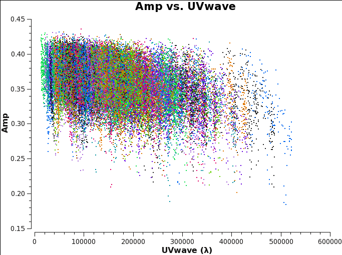
Before starting the cleaning, it makes sense to check if the emission is resolved or not by plotting amplitude as a function of uv-distance. The higher amplitudes at shorter uv-distances suggest that the source is slightly resolved.
# In CASA
plotms(vis, spw='', xaxis='uvwave', yaxis='amp', correlation='XX,YY',
       avgtime='1e8', avgchannel='1000', coloraxis='baseline')
This plot also helps us defining the cellsize needed for the task clean.
- From the plot we see that the longest baseline is 500 kilo wavelength. This means that the maximum resolution can be approximately 1/500000*206265 arcsec = 0.4 arcsec. We will use a cellsize=0.1, to oversample the beam sufficiently.
- The FWHM of the primary beam of ALMA in Band 6 is about 25 arcsec, and we want to image out to at least that extent, so we will use imsize=250.
- Since 3c286 is (nearly) a point source, we expect few clean components to be added to the model. To avoid over cleaning, set cycleniter to a small number like 10.
# In CASA
os.system('rm -rf 3c286.StokesIQUV*')
tclean(vis,
       imagename = '3c286.StokesIQUV',
       cell = ['0.1arcsec'],
       imsize = [250,250],
       deconvolver = 'clarkstokes',
       stokes = 'IQUV',
       interactive = True,
       weighting = 'briggs',
       robust = 0.5,
       niter = 500,
       pbcor = True,
       cycleniter = 10)
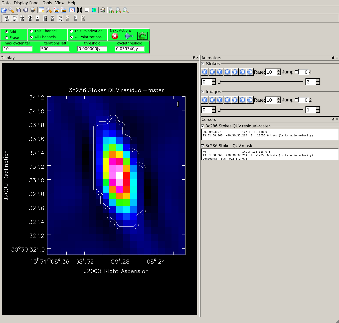
Specifying interactive=True, the tclean task brings up a viewer to show the residual clean image, where clean masks can be defined.
- Draw a tight mask around the central source, excluding the surrounding negative regions. See Figure 2. Carefully adjust the mask in each polarization plane as needed between each major cycle.
When the residuals are noise-like, the cleaning process can be finished by clicking the red X symbol. Please note that the cleaning will not start without any active mask (to activate a mask you need to double click inside the region). See First_Look_at_Imaging#First_Look_at_TCLEAN for further details on the interactive use of tclean.
Finally, note that we delete any previous versions of the output images before proceeding with the clean command. This is important, because if images with the supplied root name already exist, CASA will clean those further instead of producing new output images.
After about the 5th major cycle (90 iterations, 410 remaining), the residuals are already noise-like, so you can stop the cleaning. To view your newly cleaned image, start CARTA. If using NRAO machines, you can open a new terminal tab, cd to the working directory, then type:
# in terminal
carta --no_browser
Copy the output URL into a browser to view your CARTA session. Select and load:
3c286.StokesIQUV.image
- Fig. 3: Full Polarization Image of 3c286. Scales are NOT matched.
-
Stokes I (total intensity)
-
Stokes Q (linear polarization)
-
Stokes U (linear polarization)
-
Stokes V (circular polarization)
We can check the restoring beam by opening the File Header tool and clicking the File Information tab:
0.76326" X 0.402745", 8.34021 deg
Now draw a box in CARTA on the I plane away from the source and use the Statistics widget to determine the rms and max. Alternatively, use imstat as follows:
# In CASA
calstat = imstat(imagename='3c286.StokesIQUV.image', stokes='I', box='45,45,95,95')
rms = (calstat['rms'][0])
calstat = imstat(imagename='3c286.StokesIQUV.image', stokes='I')
peak = (calstat['max'][0])
print('>> rms in continuum image: '+str(rms))
print('>> Peak in continuum image: '+str(peak))
print('>> Dynamic range in continuum image: '+str(peak/rms))
>> rms in continuum image: 0.001051827310962827
>> Peak in continuum image: 0.2975700795650482
>> Dynamic range in continuum image: 282.90773253706163
The rms of this image is ~1.05 mJy, the peak flux density is ~298 mJy, and the dynamic range (ratio of peak/rms) is ~283.
Self-calibration
The quality of the image can be improved by applying self-calibration to the uv data. See AntennaeBand7_Imaging for details on this technique.
First, examine the model image we just created in CARTA:
3c286.StokesIQUV.model
- Fig. 4: Full Polarization Model Image of 3c286
-
Stokes I
-
Stokes Q
-
Stokes U
-
Stokes V
For self-cal, it is generally better to do a shallow initial clean than a deep clean. If your model shows too much structure, you may want to redo the previous section with a shallower clean before proceeding.
For telescopes with linear feeds such as ALMA, I and Q are determined by parallel-hand correlations XX and YY, while U and V are determined by cross-hand correlations XY and YX. Therefore, calibrations in I also affect Q. To account for this, if there is emission in Q, then Q must have a reliable model before proceeding with the self-calibration of I. A low signal in Q may result in too poor of a model. For reference, see this 2018 SISS Lecture, slide 13.
Prep
To proceed with self-calibration, first use tclean to read the model image and write model visibilities it into the MODEL column of the MS.
The model image must be closed in CARTA before being read by tclean.
# In CASA
tclean(vis,
       imagename = '3c286.StokesIQUV',
       cell = ['0.1arcsec'],
       imsize = [250,250],
       deconvolver = 'clarkstokes',
       stokes = 'IQUV',
       interactive = True,
       weighting = 'briggs',
       robust = 0.5,
       niter = 0,
       calcpsf = False,
       calcres = False,
       restoration = False,
       pbcor = True,
       savemodel = 'modelcolumn')
By default, savemodel = 'none', and the MS is opened in read-only mode. Ctrl+C can then be safely used to terminate tclean as needed. With savemodel = 'modelcolumn' (or 'virtual'), the MS will be written to, and using Ctrl+C may corrupt the MS. For the stand-alone step of reading an existing model image and writing model visibilities into the MS, choose niter = 0, calcpsf = False, calcres = False, restoration = False, and savemodel = 'modelcolumn'.
Each round of self-calibration will follow the steps:
- gaincal: create a self-calibration gain table
- plotms: examine the table
- applycal: apply the table
- tclean: make a new image
- imstat: determine image statistics
Start with a long solution interval near the length of a target scan, and decrease with each round from there.
Round 1
Now create a self-calibration gain table with gaincal:
# In CASA
os.system('rm -rf 3c286_IQUV.G1p')
gaincal(vis,
        caltable = '3c286_IQUV.G1p',
        solint = '300s',
        refantmode = 'strict',
        refant = 'DV23',
        minblperant = 4,
        calmode = 'p',
        minsnr = 4)
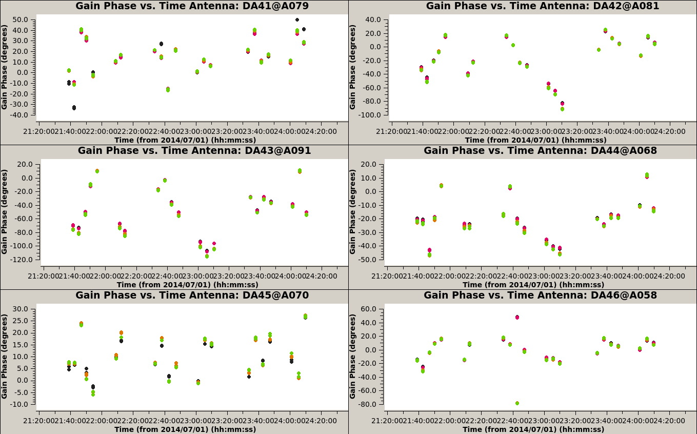
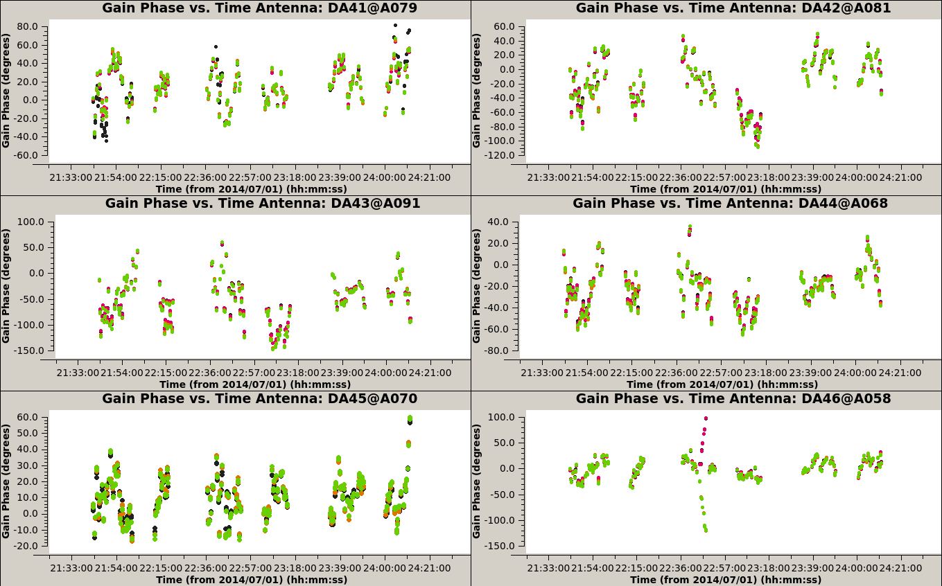
The critical parameters in this setup are solint and calmode. We will force the reference antenna to remain constant with the refantmode='strict'. We want to calculate phase solutions only so we use calmode=p and we start using solint=300s, which averages in time close to the target scan length. It is usually best to start with a large solint and then go down to the integration time if the S/N of the data permits.
To check the quality of the solutions we obtained, we plot the gains for each antenna, as function of time:
# In CASA
plotms(vis='3c286_IQUV.G1p', xaxis='time', yaxis='phase', coloraxis='spw', iteraxis='antenna', gridrows=3, gridcols=2)
Now we apply those solutions to the uv data:
# In CASA
applycal(vis, gaintable='3c286_IQUV.G1p')
Make a new image:
# In CASA
os.system('rm -rf 3c286.StokesIQUV.selfcal1*')
tclean(vis,
       imagename = '3c286.StokesIQUV.selfcal1',
       cell = ['0.1arcsec'],
       imsize = [250,250],
       deconvolver = 'clarkstokes',
       stokes = 'IQUV',
       interactive = True,
       weighting = 'briggs',
       robust = 0.5,
       pbcor = True,
       niter = 1000,
       cycleniter = 10,
       savemodel = 'modelcolumn')
Examine the image in CARTA (Fig 8) and determine new image statistics with imstat:
# In CASA
calstat = imstat(imagename='3c286.StokesIQUV.selfcal1.image', stokes='I', box='45,45,95,95')
rms = (calstat['rms'][0])
calstat = imstat(imagename='3c286.StokesIQUV.selfcal1.image', stokes='I')
peak = (calstat['max'][0])
print('>> rms in continuum image: '+str(rms))
print('>> Peak in continuum image: '+str(peak))
print('>> Dynamic range in continuum image: '+str(peak/rms))
>> rms in continuum image: 0.0002559800965899336
>> Peak in continuum image: 0.32107236981391907
>> Dynamic range in continuum image: 1254.2864624676654
The rms of this new image is ~0.256 mJy/beam, significantly lower than the value measured in the first image (1.05 mJy/beam).
Round 2
We run a second self-calibration, decreasing the solint to 30 sec, apply it to the data, and image it again:
# In CASA
os.system('rm -rf 3c286_IQUV.G2p')
gaincal(vis,
        caltable = '3c286_IQUV.G2p',
        solint = '30s',
        refantmode = 'strict',
        refant = 'DV23',
        minblperant = 4,
        calmode = 'p',
        minsnr = 4)
# In CASA
plotms(vis='3c286_IQUV.G2p', xaxis='time', yaxis='phase', coloraxis='spw', iteraxis='antenna', gridrows=3, gridcols=2)
# In CASA
applycal(vis, gaintable='3c286_IQUV.G2p')
# In CASA
os.system('rm -rf 3c286.StokesIQUV.selfcal2*')
tclean(vis,
       imagename = '3c286.StokesIQUV.selfcal2',
       cell = ['0.1arcsec'],
       imsize = [250,250],
       deconvolver = 'clarkstokes',
       stokes = 'IQUV',
       interactive = True,
       weighting = 'briggs',
       robust = 0.5,
       pbcor = True,
       niter = 1000,
       cycleniter = 10,
       savemodel = 'modelcolumn')
# In CASA
calstat = imstat(imagename='3c286.StokesIQUV.selfcal2.image', stokes='I', box='45,45,95,95')
rms = (calstat['rms'][0])
calstat = imstat(imagename='3c286.StokesIQUV.selfcal2.image', stokes='I')
peak = (calstat['max'][0])
print('>> rms in continuum image: '+str(rms))
print('>> Peak in continuum image: '+str(peak))
print('>> Dynamic range in continuum image: '+str(peak/rms))
>> rms in continuum image: 0.0002521665039442129
>> Peak in continuum image: 0.3348853290081024
>> Dynamic range in continuum image: 1328.032564873047
The rms level in this new image is ~0.252 mJy/beam. This is only slightly less than than the previous round, so we will not reduce the solint further.
Round 3
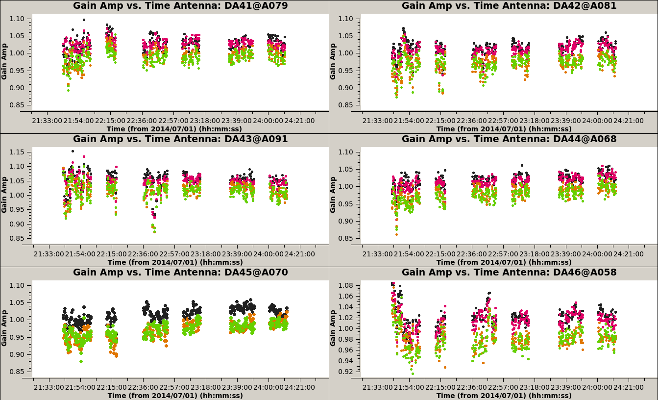
This level can be improved by a last run of self-calibration, this time solving for both amplitude and phase.
# In CASA
os.system('rm -rf 3c286_IQUV.Gap')
gaincal(vis,
        caltable = '3c286_IQUV.Gap',
        gaintable = '3c286_IQUV.G2p',
        solint = '30s',
        refantmode = 'strict',
        refant = 'DV23',
        minblperant = 4,
        calmode = 'ap',
        minsnr = 4)
# In CASA
plotms(vis='3c286_IQUV.Gap', xaxis='time', yaxis='phase', coloraxis='spw', iteraxis='antenna', gridrows=3, gridcols=2)
plotms(vis='3c286_IQUV.Gap', xaxis='time', yaxis='amp', coloraxis='spw', iteraxis='antenna', gridrows=3, gridcols=2)
# In CASA
applycal(vis, gaintable=['3c286_IQUV.G2p','3c286_IQUV.Gap'])
# In CASA
os.system('rm -rf 3c286.StokesIQUV.selfcal.ap*')
tclean(vis,
       imagename = '3c286.StokesIQUV.selfcal.ap',
       cell = ['0.1arcsec'],
       imsize = [250,250],
       deconvolver = 'clarkstokes',
       stokes = 'IQUV',
       interactive = True,
       weighting = 'briggs',
       robust = 0.5,
       pbcor = True,
       niter = 1000,
       cycleniter = 10)
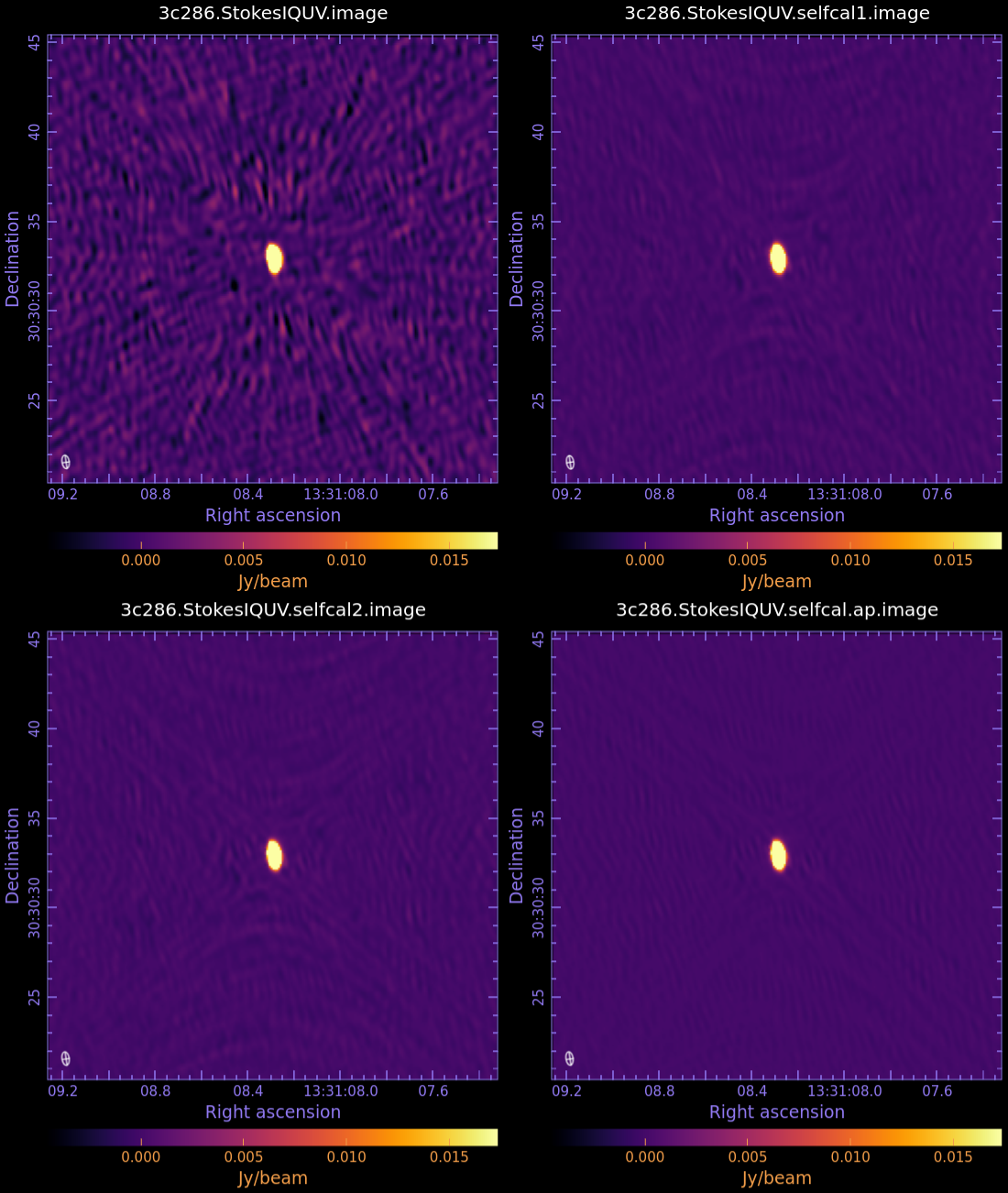
This time the first residual map shows a new bright extended component which was completely hidden by the noise in the previous images. We add a clean box around it and proceed with the clean. After 1000 cycles we stop. Examine the image in CARTA (Fig 8) and check the statistics:
# In CASA
calstat = imstat(imagename='3c286.StokesIQUV.selfcal.ap.image', stokes='I', box='45,45,95,95')
rms = (calstat['rms'][0])
calstat = imstat(imagename='3c286.StokesIQUV.selfcal.ap.image', stokes='I')
peak = (calstat['max'][0])
print('>> rms in continuum image: '+str(rms))
print('>> Peak in continuum image: '+str(peak))
print('>> Dynamic range in continuum image: '+str(peak/rms))
>> rms in continuum image: 0.0001295028028448405
>> Peak in continuum image: 0.33380603790283203
>> Dynamic range in continuum image: 2577.597013886801
The rms is 0.13 mJy, another significant decrease. We consider this result satisfying and stop the self-calibration.
Stokes images
We can extract the Stokes I, Q, U, and V images from the self-calibrated image, using the task immath:
# In CASA
os.system('rm -rf 3c286.StokesI.image*')
immath(imagename='3c286.StokesIQUV.selfcal.ap.image', outfile='3c286.StokesI.image', expr='IM0', stokes='I')

os.system('rm -rf 3c286.StokesQ.image*')
immath(imagename='3c286.StokesIQUV.selfcal.ap.image', outfile='3c286.StokesQ.image', expr='IM0', stokes='Q')

os.system('rm -rf 3c286.StokesU.image*')
immath(imagename='3c286.StokesIQUV.selfcal.ap.image', outfile='3c286.StokesU.image', expr='IM0', stokes='U')

os.system('rm -rf 3c286.StokesV.image*')
immath(imagename='3c286.StokesIQUV.selfcal.ap.image', outfile='3c286.StokesV.image', expr='IM0', stokes='V')
Now examine in CARTA and compare to Fig 3:
3c286.StokesI.image
3c286.StokesQ.image
3c286.StokesU.image
3c286.StokesV.image


We measure the statistic in each image, using the task imstat:
# In CASA
I_rms  = (imstat(imagename='3c286.StokesI.image', box='45,45,95,95')['rms'][0])
I_peak = (imstat(imagename='3c286.StokesI.image')['max'][0])

Q_rms  = (imstat(imagename='3c286.StokesQ.image', box='45,45,95,95')['rms'][0])
Q_peak = (imstat(imagename='3c286.StokesQ.image')['max'][0])

U_rms  = (imstat(imagename='3c286.StokesU.image', box='45,45,95,95')['rms'][0])
U_peak = (imstat(imagename='3c286.StokesU.image')['max'][0])

V_rms  = (imstat(imagename='3c286.StokesV.image', box='45,45,95,95')['rms'][0])
V_peak = (imstat(imagename='3c286.StokesV.image')['max'][0])

print('I_rms:  '+str(I_rms))
print('I_peak: '+str(I_peak))
print('Q_rms:  '+str(Q_rms))
print('Q_peak: '+str(Q_peak))
print('U_rms:  '+str(U_rms))
print('U_peak: '+str(U_peak))
print('V_rms:  '+str(V_rms))
print('V_peak: '+str(V_peak))
The results of the measurements for the I,Q,U,V images are reported in the table below. For details on the accuracy of polarization measurements, especially Stokes V (circular) see the Technical Handbook Section 8.7.
| I | Q | U | V | |
| rms (mJy/beam) | 0.13 | 0.02 | 0.04 | 0.02 |
| peak (mJy/beam) | 334 | 11 | 54 | 0.1 |
| dynamic range | 2569 | 550 | 1350 | 5 |
Constructing Polarization Intensity and Angle Images
We have now produced the images for all the four Stokes parameters: I, Q, U, and V. Stokes Q and U describe the linear polarization and V describes the circular polarization. Specifically, Q describes the amount of linear polarization aligned with a given axis, and U describes the amount of linear polarization at a 45 deg angle to that axis. The V parameter describes the amount of circular polarization, with the sign (positive or negative) describing the sense of the circular polarization (right- or left-hand circularly polarized).
In general, few celestial sources are expected to show circular polarization, with the notable exception of masers. Terrestrial and satellite sources are often highly circularly polarized. The V image is therefore often worth forming because any V emission could be indicative of unflagged RFI within the data (or problems with the calibration!).
Because the Q and U images both describe the amount of linear polarization, it is more common to work with a linear polarization intensity image, [math]\displaystyle{ P = \sqrt{Q^2 +U^2} }[/math]. We can also calculate the polarization position angle [math]\displaystyle{ \chi = 0.5 arctan U/Q }[/math].
In CARTA, linear polarization intensity (Plinear,POLI) and polarization position angle (Pangle,POLA) images are computed on-the-fly and can be viewed by simply toggling through the different polarization planes. This section describes how to create and save these image files in the traditional way.
The relevant task is immath; for specific examples of polarization image processing see Polarization Manipulation in the CASA Docs.
To form the linear polarization image, we combine the Q and U images using the mode='poli' option of immath.
# In CASA
os.system('rm -rf 3c286.POLI.image')
immath(outfile = '3c286.POLI.image',
       mode = 'poli',
       imagename = ['3c286.StokesQ.image','3c286.StokesU.image'],
       sigma = '0.0Jy/beam')
# In CASA
calstat = imstat(imagename='3c286.POLI.image', box='45,45,95,95')
rms = (calstat['rms'][0])
print(rms)
The measured rms is 0.04 mJy/beam.
To form the polarization position angle image we combine again the Q and U images using the mode='pola' option of immath. The Q and U images can be listed in either order. To avoid displaying the position angle of noise, we can use the polithresh parameter to set a threshold intensity of the linear polarization above which we wish to calculate the polarization angle. An appropriate level here might be the 5σ level of the polarization image, about 0.2 mJy/beam.
# In CASA
os.system('rm -rf 3c286.POLA.image')
immath(outfile = '3c286.POLA.image',
       mode = 'pola',
       imagename = ['3c286.StokesQ.image','3c286.StokesU.image'],
       polithresh = '0.2mJy/beam')
If desired, it is also possible to form the fractional linear polarization image, defined as P/I.
# In CASA
os.system('rm -rf 3c286.RATIO.image')
immath(outfile = '3c286.RATIO.image',
       mode = 'evalexpr',
       imagename = ['3c286.StokesI.image','3c286.StokesQ.image','3c286.StokesU.image'],
       expr = 'sqrt((IM1^2+IM2^2)/IM0[IM0>5e-3]^2)')
Since the total intensity image can (and hopefully does) approach zero in regions free of source emission, dividing by the total intensity can produce very high pixel values in these regions. We therefore wish to restrict our fractional polarization image to regions containing real emission, which we do by setting a threshold in the total intensity image, which in this case corresponds to five times the noise level in the Stokes I image. The computation of the polarized intensity is specified in the previous command by:
expr='sqrt((IM1^2+IM2^2)/IM0[IM0>5e-3]^2)'
with the expression in square brackets setting the threshold in IM0 (the total intensity image). Note that IM0, IM1 and IM2 correspond to the three files listed in the imagename array, in that order. In this case, the order in which the different images are specified is critical.
In order to have a dimensionless value for the ratio image, we now modify the keyword bunit in the header of the file with imhead:
# In CASA
imhead('3c286.RATIO.image', mode='put', hdkey='bunit', hdvalue='')
Image visualization and analysis
Now we can view the P (linearly polarized intensity, POLI) and [math]\displaystyle{ \chi }[/math] (polarization position angle, POLA) images in CARTA to see how the magnetic field is structured.
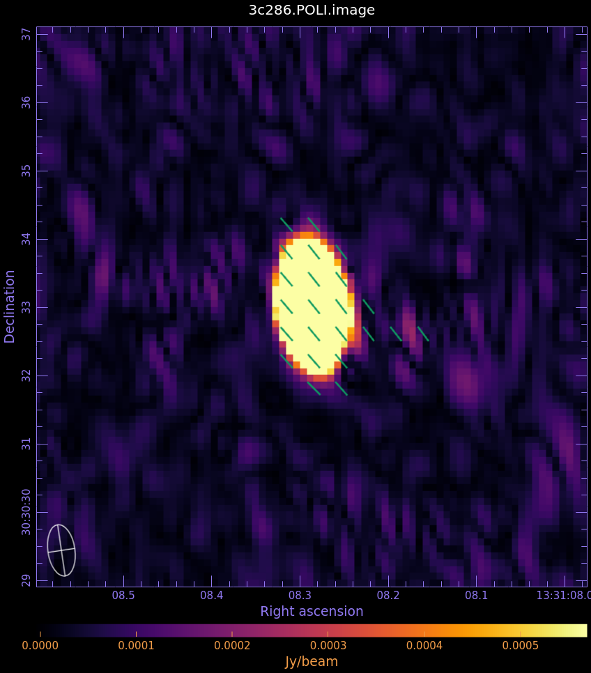
- Begin by loading the linear polarization image in CARTA: 3c286.POLI.image
- Next, append the polarization position angle image: 3c286.POLA.image
- Select the vector overlay icon from the top of the window. Set the Data Source as the POLA image, set the angular source as the current image, and set the intensity source to none, and click Apply. Images must have Spatial matching toggled on for vectors to display.
Aside: Lattice Expression Language (LEL) in CARTA
If we had we NOT set the polithresh parameter when we created the position angle ([math]\displaystyle{ \chi }[/math]) image, the position angle would have been derived for all pixels within the full IQUV image cube. To avoid plotting vectors corresponding to the position angle of pure noise, we could use CARTA to select only the regions where the polarized intensity is brighter than some threshold value. To do this, we use a LEL expression. Go to File > Append Image, click Filter, and choose "Image arithmatic." For our chosen threshold of 0.2 mJy/beam (the 5-sigma level in the P image), paste into the box the following expression:
'3c286.POLA.image'['3c286.POLI.image'>0.0002]
You can now treat this expression the same as a the polarization angle image, and use it to apply vectors. This would load the vectors only for regions where P > 0.2 mJy/beam.
If the vectors appear too densely packed on the image, we can change the spacing of the vectors. Go to Vector overlay > Averaging width. We choose 4 pixels, since there are roughly 4 pixels across our restoring beam minor axis.
For the polarization angle vector it is also possible to add a rotation. The polarization position angle as calculated is the electric vector position angle (EVPA). If we are interested in the orientation of the magnetic field, then for an optically thin source the magnetic field orientation is perpendicular to the EVPA, so we must rotate the vectors by 90 degrees. Got to Vector overlay > Styling > Rotation offset, and enter 90. We can also change the vector color.
To get quantitative information from the images, we can either use the task imstat (we already used it above) or the task imfit. The task imstat returns the statistics in a Python dictionary, from which we can read what we need in a Python variable. In this example we extract the peak value:
# In CASA
calstat = imstat(imagename='3c286.POLI.image')
print(calstat)
calstat['max'][0]
The output saved in calstat is pasted below.
{'blc': array([0, 0, 0, 0]),
 'blcf': '13:31:09.255, +30.30.20.460, Plinear, 2.3301e+11Hz',
 'flux': array([0.12833282]),
 'max': array([0.05496935]),
 'maxpos': array([125, 126,   0,   0]),
 'maxposf': '13:31:08.288, +30.30.33.060, Plinear, 2.3301e+11Hz',
 'mean': array([6.99246643e-05]),
 'medabsdevmed': array([1.40127177e-05]),
 'median': array([3.52142561e-05]),
 'min': array([1.96251136e-07]),
 'minpos': array([123,  32,   0,   0]),
 'minposf': '13:31:08.304, +30.30.23.660, Plinear, 2.3301e+11Hz',
 'npts': array([62500.]),
 'q1': array([2.24013547e-05]),
 'q3': array([5.09585843e-05]),
 'quartile': array([2.85572296e-05]),
 'rms': array([0.00093658]),
 'sigma': array([0.00093397]),
 'sum': array([4.37029152]),
 'sumsq': array([0.05482401]),
 'trc': array([249, 249,   0,   0]),
 'trcf': '13:31:07.329, +30.30.45.360, Plinear, 2.3301e+11Hz'}

Out[]: 0.05496934801340103
The task imfit finds one or more elliptical gaussian components on an image region.
# In CASA
fit_res = imfit(imagename='3c286.POLI.image')
print(fit_res)
The output saved in fit_res is pasted below.
{'converged': array([ True]),
 'deconvolved': {'component0': {'beam': {'beamarcsec': {'major': {'unit': 'arcsec',
      'value': 0.7589917778968811},
     'minor': {'unit': 'arcsec', 'value': 0.3959781229496002},
     'positionangle': {'unit': 'deg', 'value': 8.343505859375}},
    'beampixels': 34.054356973426856,
    'beamster': 8.004282680355554e-12},
   'flux': {'error': array([7.91894918e-05, 0.00000000e+00, 0.00000000e+00, 0.00000000e+00]),
    'polarisation': 'Stokes',
    'unit': 'Jy',
    'value': array([0.05750788, 0.        , 0.        , 0.        ])},
   'ispoint': False,
   'label': '',
   'peak': {'error': 0.0015593651933456223,
    'unit': 'Jy/beam',
    'value': 2.0717074748168383},
   'shape': {'direction': {'error': {'latitude': {'unit': 'arcsec',
       'value': 0.0003337666955908351},
      'longitude': {'unit': 'arcsec', 'value': 0.00010424369180659325}},
     'm0': {'unit': 'rad', 'value': -2.743927667349131},
     'm1': {'unit': 'rad', 'value': 0.5324855108720951},
     'refer': 'J2000',
     'type': 'direction'},
    'majoraxis': {'unit': 'arcsec', 'value': 0.11547921352943348},
    'majoraxiserror': {'unit': 'arcsec', 'value': 0.005617909260870177},
    'minoraxis': {'unit': 'arcsec', 'value': 0.07224425940406183},
    'minoraxiserror': {'unit': 'arcsec', 'value': 0.0028273784015794556},
    'positionangle': {'unit': 'deg', 'value': 172.82707014446243},
    'positionangleerror': {'unit': 'deg', 'value': 4.4459626695655095},
    'type': 'Gaussian'},
   'spectrum': {'channel': 0,
    'frequency': {'m0': {'unit': 'GHz', 'value': 233.00995157526424},
     'refer': 'LSRK',
     'type': 'frequency'},
    'type': 'Constant'},
   'sum': {'unit': 'Jy/beam', 'value': 1.0255171079188585}},
  'nelements': 1},
 'pixelsperarcsec': array([10., 10.]),
 'results': {'component0': {'beam': {'beamarcsec': {'major': {'unit': 'arcsec',
      'value': 0.7589917778968811},
     'minor': {'unit': 'arcsec', 'value': 0.3959781229496002},
     'positionangle': {'unit': 'deg', 'value': 8.343505859375}},
    'beampixels': 34.054356973426856,
    'beamster': 8.004282680355554e-12},
   'flux': {'error': array([7.91894918e-05, 0.00000000e+00, 0.00000000e+00, 0.00000000e+00]),
    'polarisation': 'Stokes',
    'unit': 'Jy',
    'value': array([0.05750788, 0.        , 0.        , 0.        ])},
   'ispoint': False,
   'label': '',
   'peak': {'error': 4.20449563905561e-05,
    'unit': 'Jy/beam',
    'value': 0.055859173209951776},
   'pixelcoords': array([125.25985849, 125.6072942 ]),
   'shape': {'direction': {'error': {'latitude': {'unit': 'arcsec',
       'value': 0.0003337666955908351},
      'longitude': {'unit': 'arcsec', 'value': 0.00010424369180659325}},
     'm0': {'unit': 'rad', 'value': -2.743927667349131},
     'm1': {'unit': 'rad', 'value': 0.5324855108720951},
     'refer': 'J2000',
     'type': 'direction'},
    'majoraxis': {'unit': 'arcsec', 'value': 0.767354810998606},
    'majoraxiserror': {'unit': 'arcsec', 'value': 0.0007931887998109255},
    'minoraxis': {'unit': 'arcsec', 'value': 0.40322260425386475},
    'minoraxiserror': {'unit': 'arcsec', 'value': 0.00022100562304185948},
    'positionangle': {'unit': 'deg', 'value': 8.062284889859622},
    'positionangleerror': {'unit': 'deg', 'value': 0.03223873113385978},
    'type': 'Gaussian'},
   'spectrum': {'channel': 0,
    'frequency': {'m0': {'unit': 'GHz', 'value': 233.00995157526424},
     'refer': 'LSRK',
     'type': 'frequency'},
    'type': 'Constant'},
   'sum': {'unit': 'Jy/beam', 'value': 1.0255171079188585}},
  'nelements': 1}}
To extract the flux and its error, we can read them from CASA in Python variables:
# In CASA
fluxPI  = fit_res['results']['component0']['flux']['value'][0]
errorPI = fit_res['results']['component0']['flux']['error'][0]
The flux measured in the fitted gaussian is 57.5 mJy with an error of 0.079 mJy.
We now use this method to estimate the fluxes in all the Stokes images:
# In CASA

# First we run imfit
resI = imfit(imagename='3c286.StokesI.image', box='110,110,145,145')
resQ = imfit(imagename='3c286.StokesQ.image', box='110,110,145,145')
resU = imfit(imagename='3c286.StokesU.image', box='110,110,145,145')
resV = imfit(imagename='3c286.StokesV.image', box='110,110,145,145')

# and then we extract the flux and error values for each Stokes

fluxI  = resI['results']['component0']['flux']['value'][0]
errorI = resI['results']['component0']['flux']['error'][0]

fluxQ  = resQ['results']['component0']['flux']['value'][1]
errorQ = resQ['results']['component0']['flux']['error'][1]

fluxU  = resU['results']['component0']['flux']['value'][2]
errorU = resU['results']['component0']['flux']['error'][2]

fluxV  = resV['results']['component0']['flux']['value'][3]
errorV = resV['results']['component0']['flux']['error'][3]
Now we use these values to compute polarization intensity, angle and ratio, and their errors:
# In CASA
import math

fluxPI  = math.sqrt( fluxQ**2 + fluxU**2 )
errorPI = math.sqrt( (fluxQ*errorQ)**2 + (fluxU*errorU)**2 ) / fluxPI

fluxPImjy = 1000*fluxPI
errPImjy  = 1000*errorPI

polRatio = fluxPI / fluxI
errPRat  = polRatio * math.sqrt( (errorPI/fluxPI)**2 + (errorI/fluxI)**2 )

polAngle = 0.5 * math.degrees( math.atan2(fluxU,fluxQ) )
errPA    = 0.5 * math.degrees( math.sqrt( (fluxQ*errorU)**2 + (fluxU*errorQ)**2 ) / fluxPI**2 )
The results are collected in the following table:
| Flux | err | |
| I (mJy) | 351 | 0.71 |
| Q (mJy) | 11.9 | 0.045 |
| U (mJy) | 56.2 | 0.13 |
| V (mJy) | -0.49 | -0.043 |
| Pol int (mJy) | 57.5 | 0.124 |
| P (%) | 16.4 | 0.049 |
|---|---|---|
| χ (deg) | 39.05 | 0.025 |
As you can see, the polarization intensity computed from the Q and U fluxes is the same as the one extracted from the polarization image (as it should be!).
Note that the uncertainties quoted above are purely statistical. The systematic errors will be larger, and include (but are not limited to) any net bias in the position angle of the linear feeds in the antennas, the details of different observations (at what parallactic angles, etc.), and other data quality variations (including source structure). We conservatively estimate the position angle uncertainty to be ± 2º.
Finally, we compare with previous results from IRAM and CARMA: Agudo et al. (2012) presented the results of single-dish millimeter measurements of 3c286 with the IRAM 30m Telescope. Their observations at 1 mm (229 GHz) and 3 mm (86 GHz) produced the following results:
| 1 mm | 3 mm | |
| P (%) | 14.4 ± 1.8 | 13.5 ± 0.3 |
| χ (deg) | 33.1 ± 5.7 | 37.3 ± 0.8 |
CARMA Memo 64 and Hull & Plambeck 2015 (JAI) and report interferometric polarization data of 3c286 taken with CARMA at 1 mm (225 GHz). Their results are as follows:
| 1 mm | |
| χ (deg) | 39.2 ± 1.0 |
Export images in fits format
To get all images in fits format you need to use the task exportfits. Close all images in CARTA before this.
You can add the parameters imagename (the input image) and fitsimage (the name of the output image) one by one or you can run a python cycle over all the images:
# In CASA
import glob

imagenames=glob.glob("*image")

for name in imagenames:
    exportfits(imagename=name, fitsimage=name+'.fits')
