VLBA Basic Spectral Line Tutorial DRAFT: Difference between revisions
No edit summary |
|||
| (36 intermediate revisions by the same user not shown) | |||
| Line 6: | Line 6: | ||
== Overview == | == Overview == | ||
This CASA Guide describes the procedure for calibrating a phase-referenced VLBA observation of methanol masers in W3OH. The data were taken specifically for this tutorial. The observation made use of the DDC observing personality, using dual polarization with one spectral | This CASA Guide describes the procedure for calibrating a phase-referenced VLBA observation of methanol masers in W3OH. The data were taken specifically for this tutorial. The observation made use of the DDC observing personality, using dual polarization with one spectral window in each polarization. The spectral window has a bandwidth of 32 MHz divided into 640 spectral channels centered at 6668 MHz for the methanol maser line. In addition, there is a "zoom" band file with very high spectral resolution centered on the maser line. The methanol maser line itself has a rest frequency of 6668.5192 MHz (e.g., [https://ui.adsabs.harvard.edu/abs/2004A%26A...428.1019M/abstract Muller, Menten & Mader 2004]). | ||
This tutorial will focus on calibrating the data and creating a continuum (Stokes I) image of the phase reference calibrator and image cubes of some of the stronger the masers in W3OH. | This tutorial will focus on calibrating the data and creating a continuum (Stokes I) image of the phase reference calibrator and image cubes of some of the stronger the masers in W3OH. | ||
| Line 21: | Line 21: | ||
If your observation involves any of the above, you should use [http://www.aips.nrao.edu/index.shtml AIPS] to calibrate your data. | If your observation involves any of the above, you should use [http://www.aips.nrao.edu/index.shtml AIPS] to calibrate your data. | ||
<b>A note on pre-DiFX data:</b> Starting with CASA 6.6.4, VLBA data correlated with the hardware correlator (prior to December 2009) can be imported into CASA Measurement Sets with [https://casadocs.readthedocs.io/en/v6.6. | <b>A note on pre-DiFX data:</b> Starting with CASA 6.6.4, VLBA data correlated with the hardware correlator (prior to December 2009) can be imported into CASA Measurement Sets with [https://casadocs.readthedocs.io/en/v6.6.5/api/tt/casatasks.data.importfitsidi.html importfitsidi]. However, users should take great care in using CASA to calibrate these data because the data weights may not be correct, especially for the oldest data and data with the Hanning taper applied. Warning messages will appear for data with the Hanning taper applied and some other known problems, but not every case has been tested. | ||
<b>A note on Earth Orientation Parameter corrections:</b> Starting with CASA 6.6.5 (Fall 2024), it | <b>A note on Earth Orientation Parameter corrections:</b> Starting with CASA 6.6.5 (Fall 2024), it is possible to correct the Earth Orientation Parameters (EOP) in a VLBA observation. Unlike with AIPS, CASA users will need to download the EOP file themselves. These files can be obtained from NASA using the following command: curl -u anonymous:<your-email-address> --ftp-ssl ftp://gdc.cddis.eosdis.nasa.gov/vlbi/gsfc/ancillary/solve_apriori/usno_finals.erp > /<path>/<to>/<file>/usno_finals.erp | ||
<b>A note on VLBA+Y1 observations:</b> It is currently possible to calibrate VLBA+Y1 (VLBA and single VLA antenna) in CASA. Any data taken after 2022 July 06 should work with minimal extra steps (namely, checking that the Y1 antenna diameter is correct). VLBA+Y1 data observed prior to 2022 July 06 may not include the system temperature and/or gain curve values need for calibration. For these data sets, refer to [https://library.nrao.edu/public/memos/vlba/sci/VLBAS_39.pdf VLBA Scientific Memo 39] for details on how to prepare the data for calibration in either CASA or AIPS. | <b>A note on VLBA+Y1 observations:</b> It is currently possible to calibrate VLBA+Y1 (VLBA and single VLA antenna) in CASA. Any data taken after 2022 July 06 should work with minimal extra steps (namely, checking that the Y1 antenna diameter is correct). VLBA+Y1 data observed prior to 2022 July 06 may not include the system temperature and/or gain curve values need for calibration. For these data sets, refer to [https://library.nrao.edu/public/memos/vlba/sci/VLBAS_39.pdf VLBA Scientific Memo 39] for details on how to prepare the data for calibration in either CASA or AIPS. | ||
<b><span style="color:#FF0000"> Mac OS 13 and OS 14 WARNING: </span></b>The CASA Viewer will not work on Mac OS 13, OS 14, or later. The [https://casadocs.readthedocs.io/en/v6. | <b><span style="color:#FF0000"> Mac OS 13 and OS 14 WARNING: </span></b>The CASA Viewer will not work on Mac OS 13, OS 14, or later. The [https://casadocs.readthedocs.io/en/v6.6.5/api/tt/casatasks.imaging.tclean.html tclean] task relies on the CASA Viewer for interactive cleaning. So, users with Mac OS 13, OS 14, or newer will not be able to make their images interactively in CASA. Because interactive cleaning is extremely important for creating image cubes from VLBA spectral line observations, users running Mac OS 13, OS 14, or later are strongly encouraged to use an alternate software package to create their images ([http://www.aips.nrao.edu/index.shtml AIPS]). Alternatively, Mac users can request access to Linux-based NRAO computing resources by submitting a [https://help.nrao.edu helpdesk] ticket (in the Department field, select "VLA/GBT/VLBA Archive and Data Retrieval" and request a guest account to calibrate and image VLBA data). | ||
== How to Use This CASA Guide == | == How to Use This CASA Guide == | ||
| Line 103: | Line 103: | ||
Before beginning our data reduction, we must start CASA. If you have not used CASA before, some helpful tips are available on the [[Getting Started in CASA]] page. Remember to start CASA in the directory containing the observation data. | Before beginning our data reduction, we must start CASA. If you have not used CASA before, some helpful tips are available on the [[Getting Started in CASA]] page. Remember to start CASA in the directory containing the observation data. | ||
Once you have CASA up and running, it is time to get the data into a format that CASA can use. Unlike VLA data, a VLBA observation is only available as a FITS-IDI file and cannot be downloaded as a CASA Measurement Set. So, the first step in calibrating a VLBA observation with CASA is to create a Measurement Set from the FITS-IDI file. To do this, we will use the task [https://casadocs.readthedocs.io/en/v6. | Once you have CASA up and running, it is time to get the data into a format that CASA can use. Unlike VLA data, a VLBA observation is only available as a FITS-IDI file and cannot be downloaded as a CASA Measurement Set. So, the first step in calibrating a VLBA observation with CASA is to create a Measurement Set from the FITS-IDI file. To do this, we will use the task [https://casadocs.readthedocs.io/en/v6.6.5/api/tt/casatasks.data.importfitsidi.html importfitsidi]: | ||
<source lang="python"> | <source lang="python"> | ||
| Line 110: | Line 110: | ||
</source> | </source> | ||
The ''scanreindexgap_s'' parameter is used to reconstruct scan boundaries in those cases where sources do not change between scans. In general, it is good to set ''scanreindexgap_s'' to some non-zero number to help CASA properly organize the scan list. The recommended value is 15 seconds, but smaller values may work as well (although you probably don't want to go much shorter than about 5 seconds). If you find that the resulting MS contains too few scans, run [https://casadocs.readthedocs.io/en/v6. | The ''scanreindexgap_s'' parameter is used to reconstruct scan boundaries in those cases where sources do not change between scans. In general, it is good to set ''scanreindexgap_s'' to some non-zero number to help CASA properly organize the scan list. The recommended value is 15 seconds, but smaller values may work as well (although you probably don't want to go much shorter than about 5 seconds). If you find that the resulting MS contains too few scans, run [https://casadocs.readthedocs.io/en/v6.6.5/api/tt/casatasks.data.importfitsidi.html importfitsidi] again with ''scanreindexgap_s'' set to a smaller number. If your MS has too many scans, especially multiple scans on the same source when you think it should just be one scan, run [https://casadocs.readthedocs.io/en/v6.6.5/api/tt/casatasks.data.importfitsidi.html importfitsidi] again with ''scanreindexgap_s'' set to a larger number. | ||
<b> NOTE: </b>You may see warnings in the CASA window like "Table not yet implemented" and "Keyword has wrong data type". This is normal behavior for VLBA data and due to the fact that CASA does not yet handle the pulse-cal tone data in the FTIS-IDI file. Just ignore them. However, do not ignore any SEVERE warnings, as these can indicate there are serious problems with the data. | <b> NOTE: </b>You may see warnings in the CASA window like "Table not yet implemented" and "Keyword has wrong data type". This is normal behavior for VLBA data and due to the fact that CASA does not yet handle the pulse-cal tone data in the FTIS-IDI file. Just ignore them. However, do not ignore any SEVERE warnings, as these can indicate there are serious problems with the data. | ||
| Line 120: | Line 120: | ||
=== The Observation Summary === | === The Observation Summary === | ||
It will be useful later to have the basic information about the observation. The task [https://casadocs.readthedocs.io/en/v6. | It will be useful later to have the basic information about the observation. The task [https://casadocs.readthedocs.io/en/v6.6.5/api/tt/casatasks.information.listobs.html listobs] will return a list of all the scans, the sources observed, which stations were used, and the frequency setup. It is possible to run [https://casadocs.readthedocs.io/en/v6.6.5/api/tt/casatasks.information.listobs.html listobs] in two ways: printing information in the CASA logger, or saving the information to a file. | ||
To simply display the information in the CASA logger: | To simply display the information in the CASA logger: | ||
| Line 128: | Line 128: | ||
</source> | </source> | ||
You should see the [https://casadocs.readthedocs.io/en/v6. | You should see the [https://casadocs.readthedocs.io/en/v6.6.5/api/tt/casatasks.information.listobs.html listobs] output in the CASA logger window: | ||
<pre style="background-color: #fffacd;"> | <pre style="background-color: #fffacd;"> | ||
| Line 302: | Line 302: | ||
</pre> | </pre> | ||
<b>NOTE:</b> You can also assign the [https://casadocs.readthedocs.io/en/v6. | <b>NOTE:</b> You can also assign the [https://casadocs.readthedocs.io/en/v6.6.5/api/tt/casatasks.information.listobs.html listobs] output to a python dictionary (e.g., "obs_dict") by typing "obs_dict = listobs(vis='tl016g.ms')". | ||
It is usually useful to have a copy of the [https://casadocs.readthedocs.io/en/v6. | It is usually useful to have a copy of the [https://casadocs.readthedocs.io/en/v6.6.5/api/tt/casatasks.information.listobs.html listobs] output in a file that you can refer to later. To save the [https://casadocs.readthedocs.io/en/v6.6.5/api/tt/casatasks.information.listobs.html listobs] output to a file named "tl016b_listobs.txt", run [https://casadocs.readthedocs.io/en/v6.6.5/api/tt/casatasks.information.listobs.html listobs] again with ''listfile='tl016g_listobs.txt'''. | ||
<source lang="python"> | <source lang="python"> | ||
#In CASA | #In CASA | ||
| Line 322: | Line 322: | ||
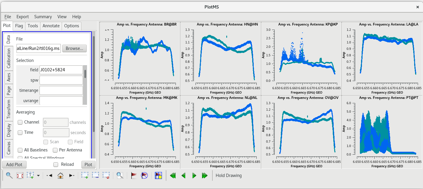
[[File:vlba_SpectralLine_W3OH_scan14_ampVfreq.png|300px|right|thumb|Figure 1: Plot of amplitude vs. frequency for scan 14 on W3OH. Data for each antenna is plotted separately. Notice the large spike near the center of the band on each antenna. Also, notice that Pie Town appears to suffer from major RFI problems.]] | [[File:vlba_SpectralLine_W3OH_scan14_ampVfreq.png|300px|right|thumb|Figure 1: Plot of amplitude vs. frequency for scan 14 on W3OH. Data for each antenna is plotted separately. Notice the large spike near the center of the band on each antenna. Also, notice that Pie Town appears to suffer from major RFI problems.]] | ||
Because this observation was looking for a strong maser line, one of the first things we should do is check that an emission line was detected from our target source. We will do this by using [https://casadocs.readthedocs.io/en/v6. | Because this observation was looking for a strong maser line, one of the first things we should do is check that an emission line was detected from our target source. We will do this by using [https://casadocs.readthedocs.io/en/v6.6.5/api/tt/casaplotms.plotms.html plotms] to plot amplitude vs frequency for the target source, W3OH. We will pick a single scan to plot because it will help plotms run faster. Looking at the tl016g_listobs.txt file we made above, we can see that W3OH was the target of scans 4, 6, 8, 10, 12, 14, etc. One of my favorite hockey players, Brendan Shanahan of the Detroit Red Wings, wore jersey number 14, so we'll use that scan. As an extra shortcut, we will plot all of the antennas simultaneously using the ''gridrows'' and ''gridcols'' parameters. | ||
<source lang="python"> | <source lang="python"> | ||
| Line 342: | Line 342: | ||
You should see that the RFI is present in each scan. This is bad news for us. Because the RFI is persistent and so close to the maser line, we will probably need to flag the Pie Town antenna. We were already missing Fort Davis and Saint Croix, so losing Pie Town will bring us down to only seven stations. | You should see that the RFI is present in each scan. This is bad news for us. Because the RFI is persistent and so close to the maser line, we will probably need to flag the Pie Town antenna. We were already missing Fort Davis and Saint Croix, so losing Pie Town will bring us down to only seven stations. | ||
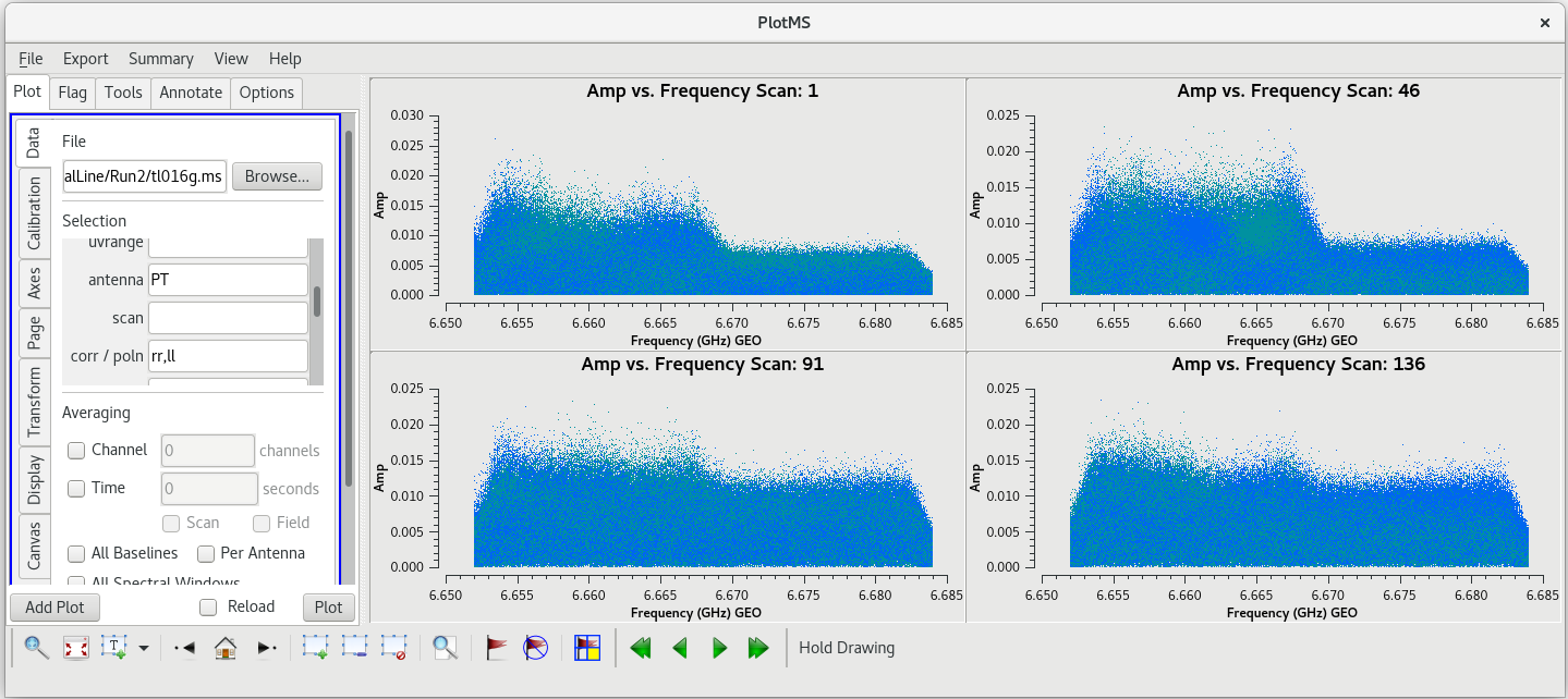
Before we lose all hope in Pie Town, let's see if the RFI is only on the autocorrelations or if it also impacts the cross correlations. To plot the cross correlations to Pie Town, we will use the ''antenna'' parameter in [https://casadocs.readthedocs.io/en/v6. | Before we lose all hope in Pie Town, let's see if the RFI is only on the autocorrelations or if it also impacts the cross correlations. To plot the cross correlations to Pie Town, we will use the ''antenna'' parameter in [https://casadocs.readthedocs.io/en/v6.6.5/api/tt/casaplotms.plotms.html plotms]. | ||
<source lang="python"> | <source lang="python"> | ||
| Line 349: | Line 349: | ||
</source> | </source> | ||
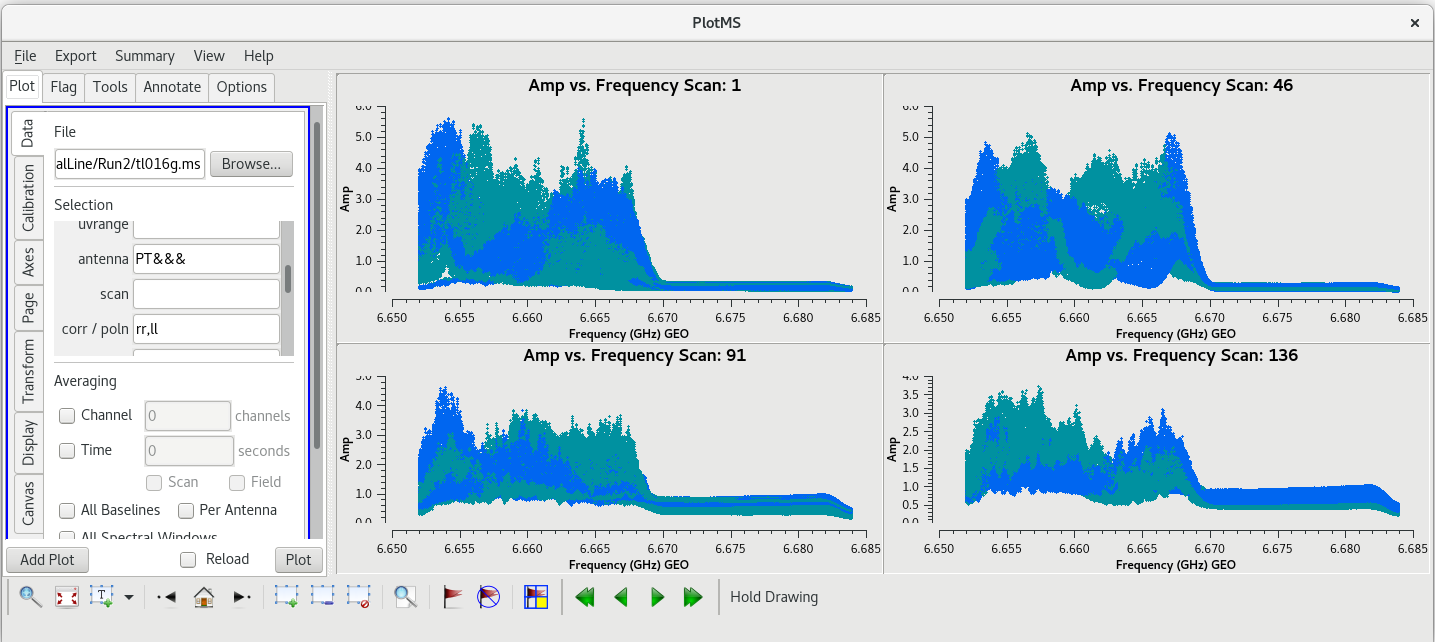
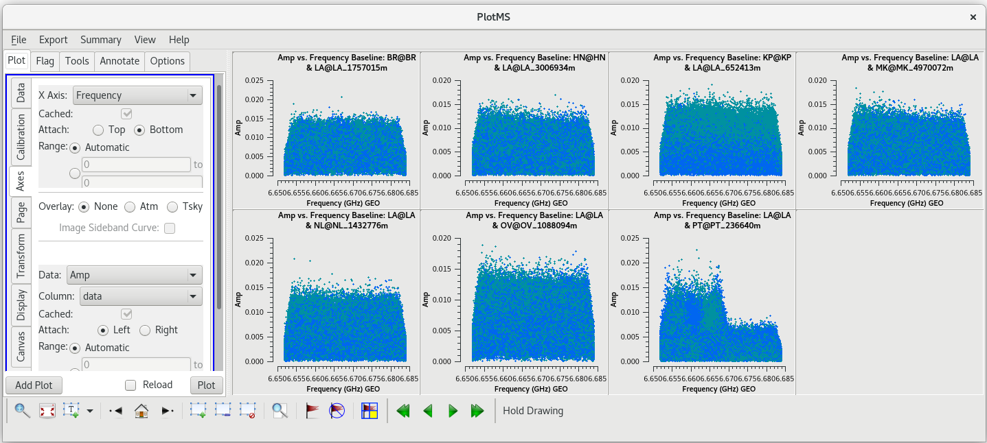
You can see that the RFI does indeed cause problems on the corss correlations, but not nearly as bad as on the autocorrelations. If you want to see just the PT autocorrelations, set ''antenna='PT&&&''' in the [https://casadocs.readthedocs.io/en/v6. | You can see that the RFI does indeed cause problems on the corss correlations, but not nearly as bad as on the autocorrelations. If you want to see just the PT autocorrelations, set ''antenna='PT&&&''' in the [https://casadocs.readthedocs.io/en/v6.6.5/api/tt/casaplotms.plotms.html plotms] GUI and click "Plot". | ||
{| | {| | ||
| Line 361: | Line 361: | ||
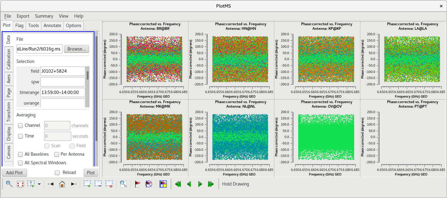
VLBA calibration makes use of a reference antenna: one antenna that all other antennas can be referenced to when generating solutions. Usually, you will want to use one of the more central stations: FD, KP, LA, or PT. For this observation, FD was missing (see the Observing Log), and we know PT had RFI issues. So, our choices are down to KP and LA. | VLBA calibration makes use of a reference antenna: one antenna that all other antennas can be referenced to when generating solutions. Usually, you will want to use one of the more central stations: FD, KP, LA, or PT. For this observation, FD was missing (see the Observing Log), and we know PT had RFI issues. So, our choices are down to KP and LA. | ||
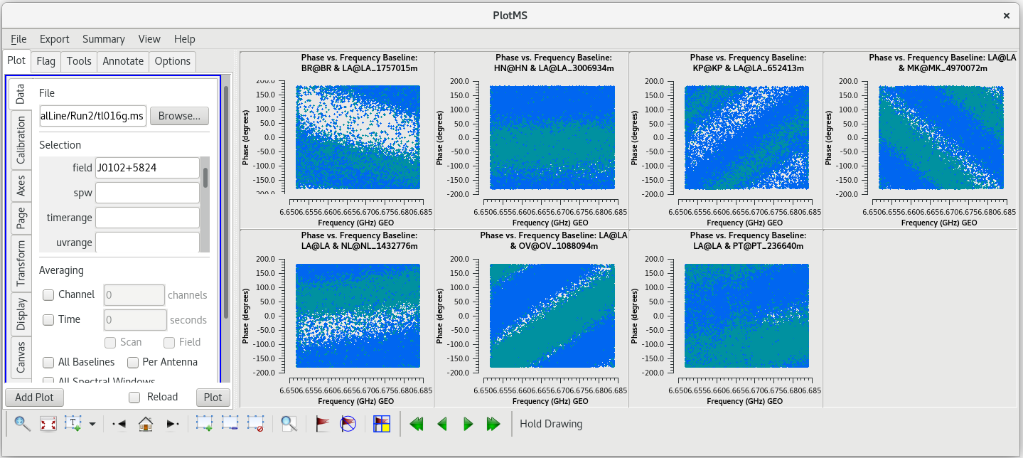
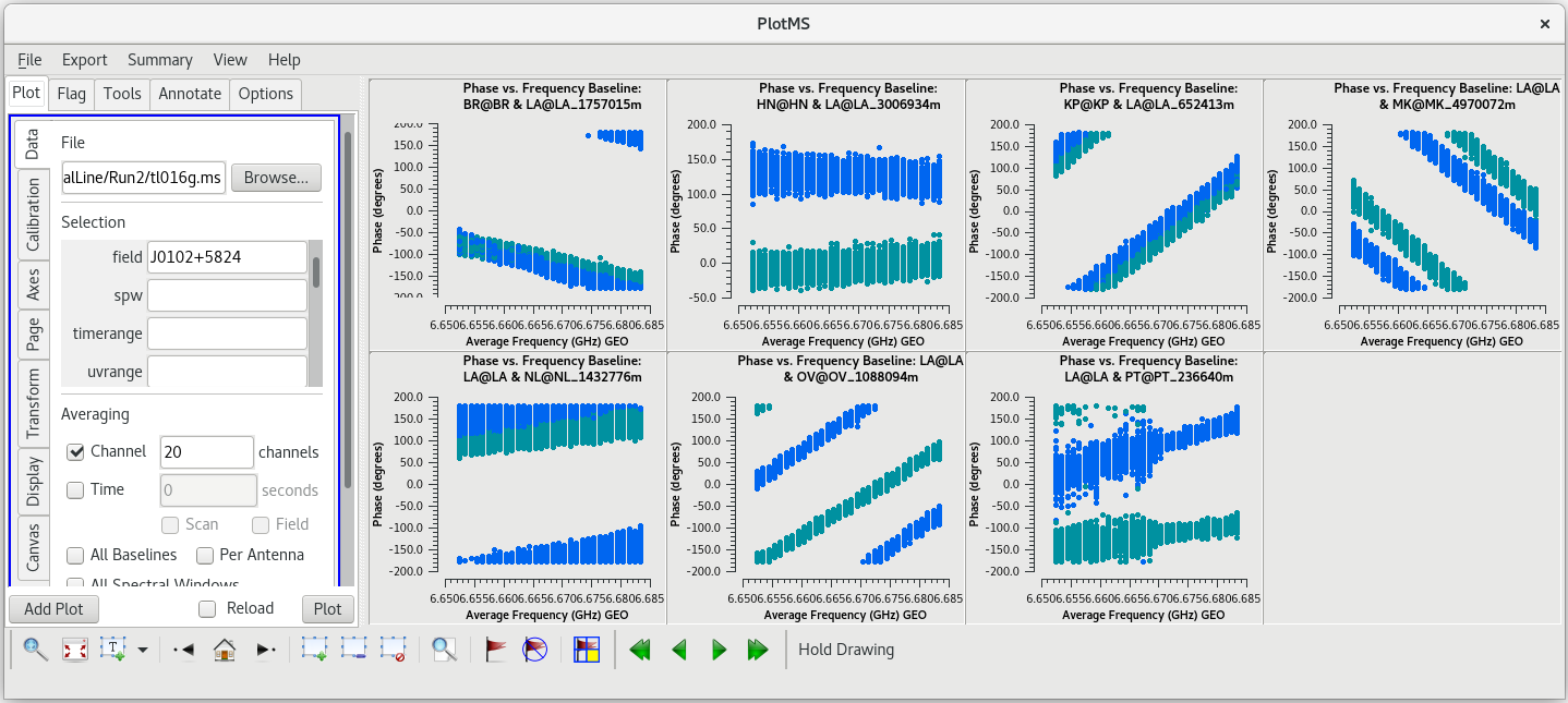
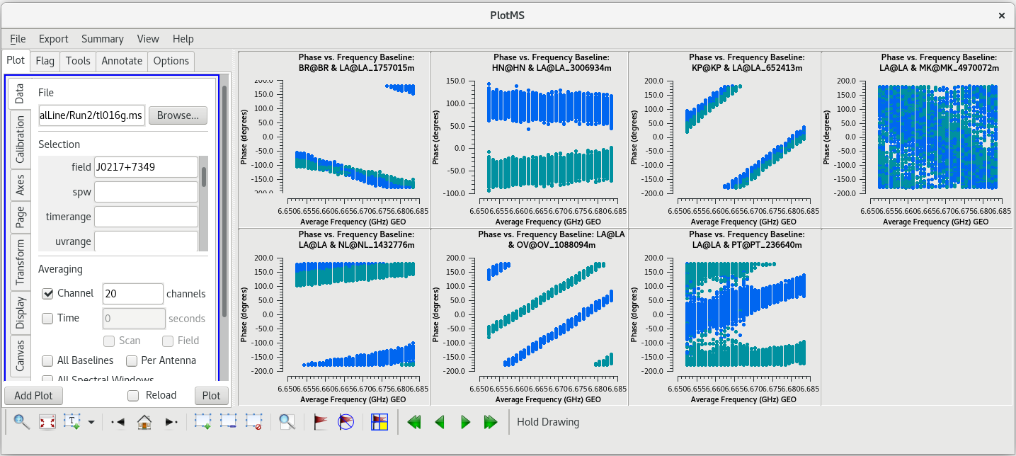
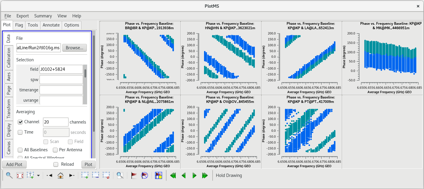
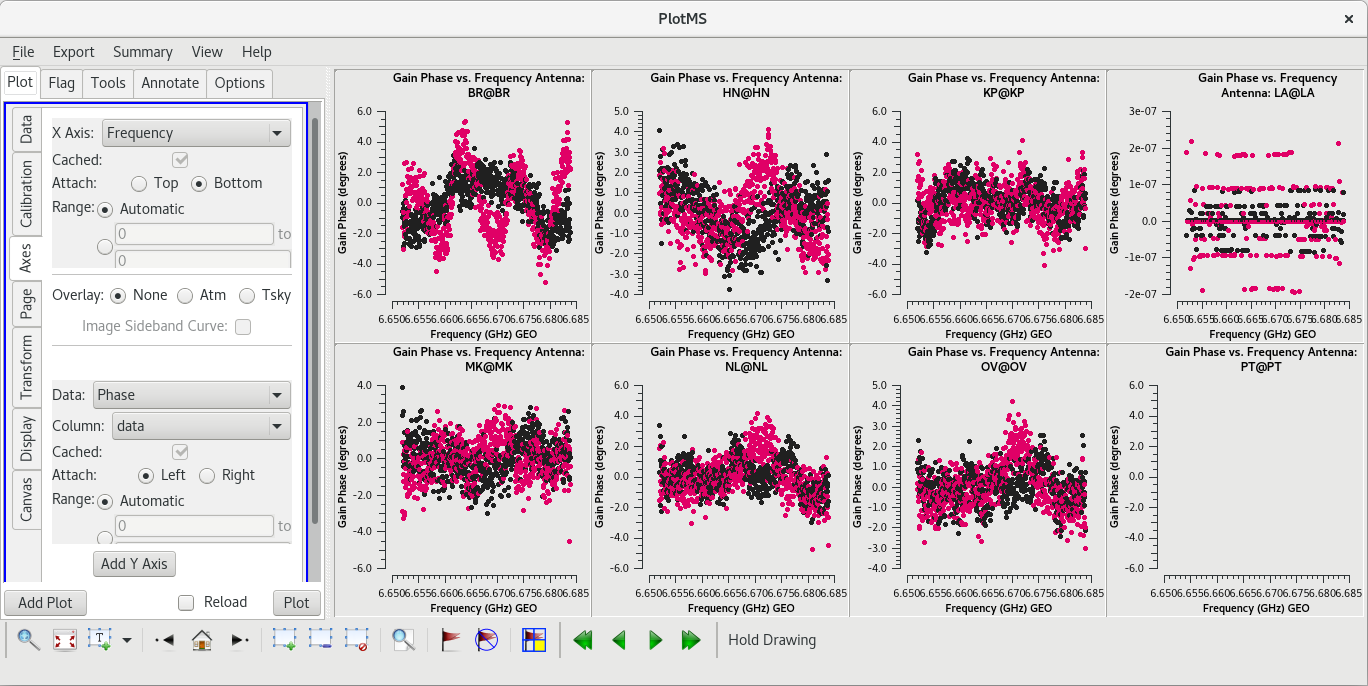
To determine which is the best to use as the reference antenna, use [https://casadocs.readthedocs.io/en/v6. | To determine which is the best to use as the reference antenna, use [https://casadocs.readthedocs.io/en/v6.6.5/api/tt/casaplotms.plotms.html plotms] to plot phase vs frequency for a single scan on a bright source (usually the fringe finder or bandpass calibrator). For this observation, use the second scan on J0102+5824, which is scan 46 from the [https://casadocs.readthedocs.io/en/v6.6.5/api/tt/casatasks.information.listobs.html listobs] output. We start with scan 46 because it is near the middle of our observation, so J0102+5824 should be at relatively high elevations at all stations during that scan. We will look at all the baselines to LA first. | ||
<source lang="python"> | <source lang="python"> | ||
| Line 427: | Line 427: | ||
In the VLBA Basic Phase-referencing tutorial, the first flagging step is to "quack" the date (flag the first and last few seconds of each scan). However, we did not notice any real problems at the begining or end of scan 46. So, we probably do not need to quack these data. | In the VLBA Basic Phase-referencing tutorial, the first flagging step is to "quack" the date (flag the first and last few seconds of each scan). However, we did not notice any real problems at the begining or end of scan 46. So, we probably do not need to quack these data. | ||
=== Flagging Problem | === Flagging Problem Times === | ||
The first scan of VLBA observations often have some minor problems during the first few seconds. We should take a look at scan 1 to see if this observation has any such problems. | The first scan of VLBA observations often have some minor problems during the first few seconds. We should take a look at scan 1 to see if this observation has any such problems. | ||
| Line 448: | Line 448: | ||
</source> | </source> | ||
If you kept the [https://casadocs.readthedocs.io/en/v6. | If you kept the [https://casadocs.readthedocs.io/en/v6.6.5/api/tt/casaplotms.plotms.html plotms] window open, you can check the "Reload" box and then click "Plot" to update the plots. You should see that the low points are now gone. | ||
=== Flagging Problem Antennas === | === Flagging Problem Antennas === | ||
| Line 454: | Line 454: | ||
We know from our inspection of the fringe finders that PT has some major RFI near the maser line. Therefore, we should not include PT in our calibration. In fact, we should not use PT at all since it may be contributing bad data and/or noise to our observations. | We know from our inspection of the fringe finders that PT has some major RFI near the maser line. Therefore, we should not include PT in our calibration. In fact, we should not use PT at all since it may be contributing bad data and/or noise to our observations. | ||
Flag the PT antenna for the entire observation by using the [https://casadocs.readthedocs.io/en/v6. | Flag the PT antenna for the entire observation by using the [https://casadocs.readthedocs.io/en/v6.6.5/api/tt/casatasks.flagging.flagdata.html flagdata] command | ||
<source lang="python"> | <source lang="python"> | ||
#In CASA | #In CASA | ||
| Line 462: | Line 462: | ||
=== Automated Flagging === | === Automated Flagging === | ||
The | The [https://casadocs.readthedocs.io/en/v6.6.5/api/tt/casatasks.flagging.flagdata.html flagdata] task includes a useful automated flagging mode known as "TFCrop". For more details on using the automated TFcrop mode, see the [https://casaguides.nrao.edu/index.php?title=VLA_CASA_Flagging-CASA6.2.0#TFCrop VLA CASA Flagging] topical tutorial. Because this is a spectral line data set, we want to limit the automatic flagging to only the time domain. We will also avoid flagging on the maser lines, just to be extra careful (the maser lines are so bright that a small amount of RFI will not make any real difference). | ||
To begin, you just want to get a feel for what TFCrop will do to the data, which means you should set ''action='calculate' ''. | To begin, you just want to get a feel for what TFCrop will do to the data, which means you should set ''action='calculate' ''. | ||
| Line 470: | Line 470: | ||
</source> | </source> | ||
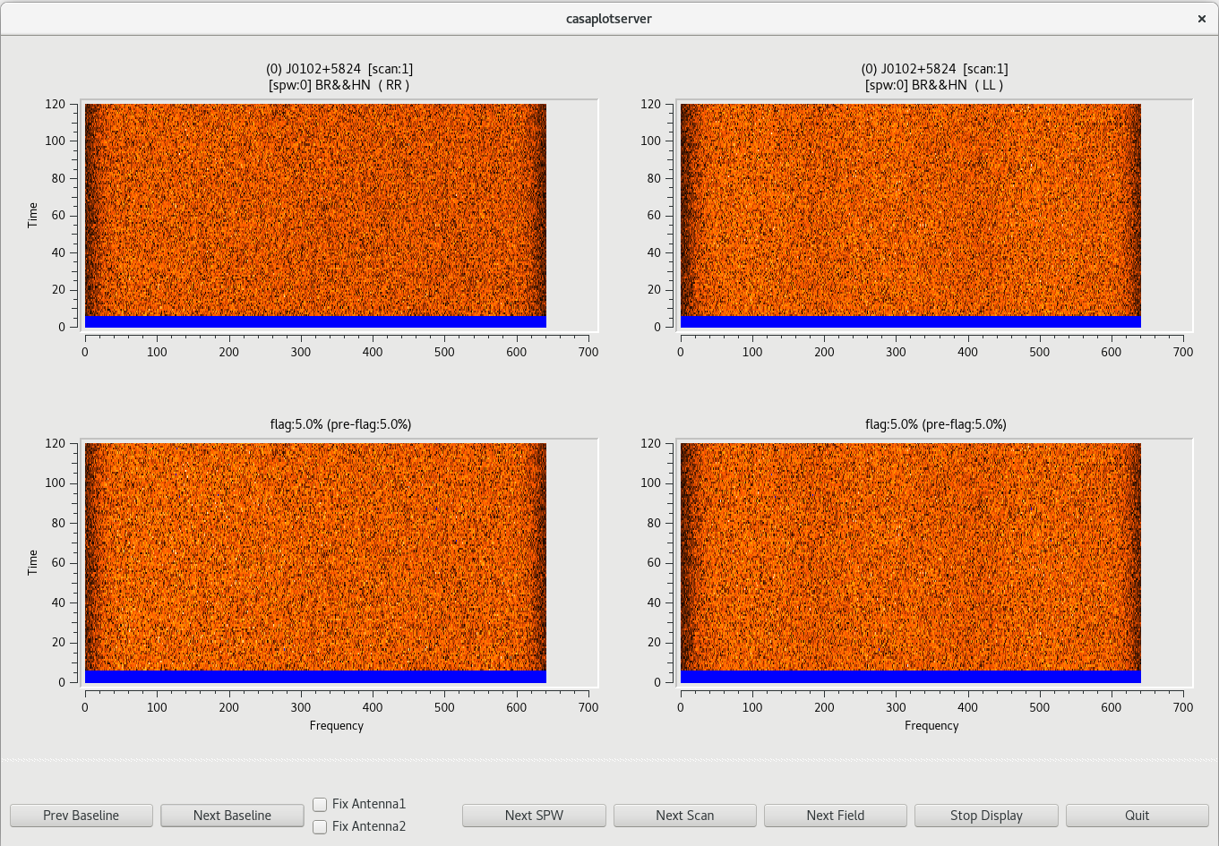
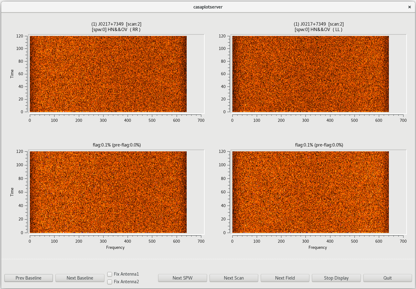
This will open a new window with a GUI. The top row of the GUI will display the data as it currently is. The bottom row shows what the data will look like after the flags are applied (blue regions are flagged). Step through the antennas by clicking "Next Baseline". | This will open a new window with a GUI. The top row of the GUI will display the data as it currently is. The bottom row shows what the data will look like after the flags are applied (blue regions are flagged). Step through the antennas by clicking "Next Baseline". Step through at least a few scans by clicking "Next Scan". With ''timecutoff=4.0'', it should really only flag those data points that are 4-times the standard deviation in the time dimension. This should be sufficient to remove the worst of the time-dependent RFI in our observation. For all of the baselines in the first scan, you will notice that there is a blue band at the bottom of the plots. This is the result of flagging the first 12 seconds of scan 1 above. Click on "Next Scan" to take a look at the data on J0217+7349. Stepping through the baselines on this scan, you should see that not much gets flagged. However, some very bright points are found and flagged by the code, which is exactly what we want to see. Take some time to look at some scans on the phase reference calibrator, J0306+6243, as well. | ||
{| | {| | ||
| Line 477: | Line 477: | ||
|} | |} | ||
To generate the flags, we will need to run [https://casadocs.readthedocs.io/en/v6. | To generate the flags, we will need to run [https://casadocs.readthedocs.io/en/v6.6.5/api/tt/casatasks.flagging.flagdata.html flagdata] again with ''action='apply' ''. | ||
<source lang="python"> | <source lang="python"> | ||
#In CASA | #In CASA | ||
| Line 491: | Line 491: | ||
As telescope arrays become larger and more complex, automated flagging will become the primary means of excluding bad data (just look at what ALMA does). However, the current VLBA is still small enough and the data rates are low enough that inspecting and flagging data oneself is not too painful. | As telescope arrays become larger and more complex, automated flagging will become the primary means of excluding bad data (just look at what ALMA does). However, the current VLBA is still small enough and the data rates are low enough that inspecting and flagging data oneself is not too painful. | ||
You can look for obvious bad data using [https://casadocs.readthedocs.io/en/v6. | You can look for obvious bad data using [https://casadocs.readthedocs.io/en/v6.6.5/api/tt/casaplotms.plotms.html plotms]. Be aware that while you can flag data in [https://casadocs.readthedocs.io/en/v6.6.5/api/tt/casaplotms.plotms.html plotms], a major drawback to using [https://casadocs.readthedocs.io/en/v6.6.5/api/tt/casaplotms.plotms.html plotms] to flag data is that it makes undoing flags very difficult. The preferred method of flagging by hand is to identify the bad data with [https://casadocs.readthedocs.io/en/v6.6.5/api/tt/casaplotms.plotms.html plotms], and then generate the flags with [https://casadocs.readthedocs.io/en/v6.6.5/api/tt/casatasks.flagging.flagdata.html flagdata]. It is recommended to be somewhat careful with flagging early on in the calibration process and only flag those data points that are obviously bad. | ||
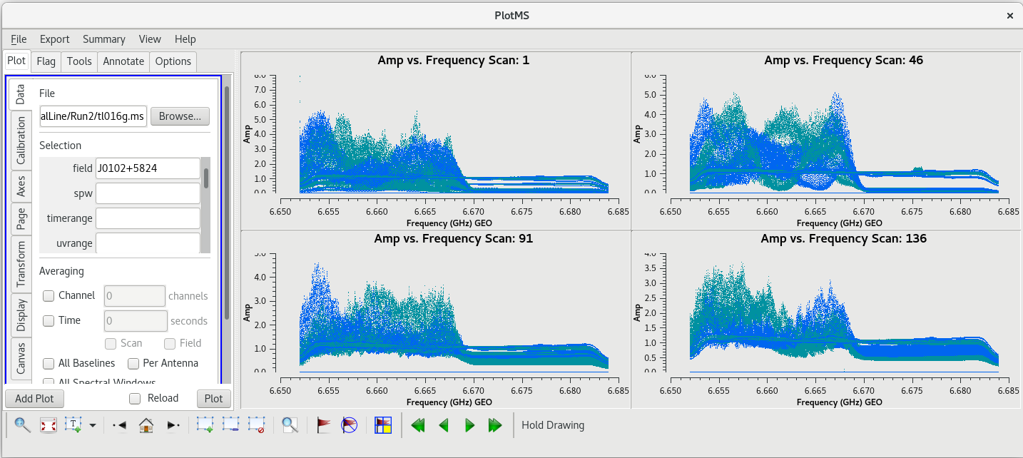
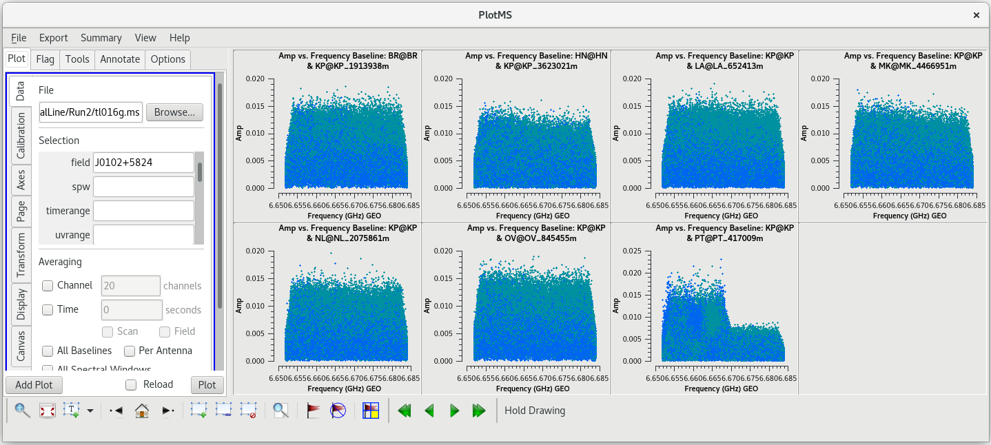
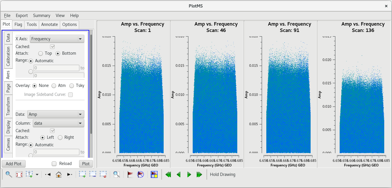
Let's start by taking a look at all the scans on our fringe finder and bandpass calibrator, J0102+5824. We will plot amplitude vs frequency for all four scans. We will aviod plotting the autocorrelations by setting ''antenna='*&*''' | Let's start by taking a look at all the scans on our fringe finder and bandpass calibrator, J0102+5824. We will plot amplitude vs frequency for all four scans. We will aviod plotting the autocorrelations by setting ''antenna='*&*''' | ||
| Line 502: | Line 502: | ||
You should see that this looks pretty good. The final scan (136) may look a little low, but pay close attention to the y-axis values and you will notice that it is actually about the same as the other scans. | You should see that this looks pretty good. The final scan (136) may look a little low, but pay close attention to the y-axis values and you will notice that it is actually about the same as the other scans. | ||
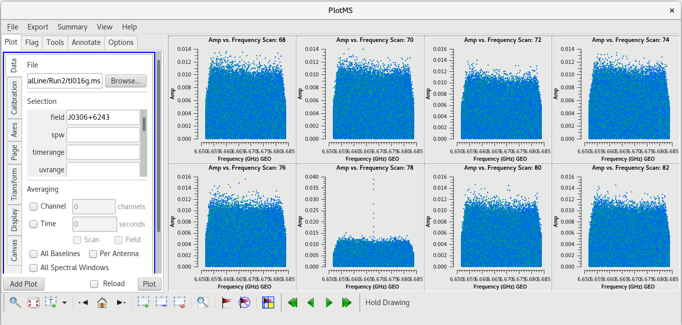
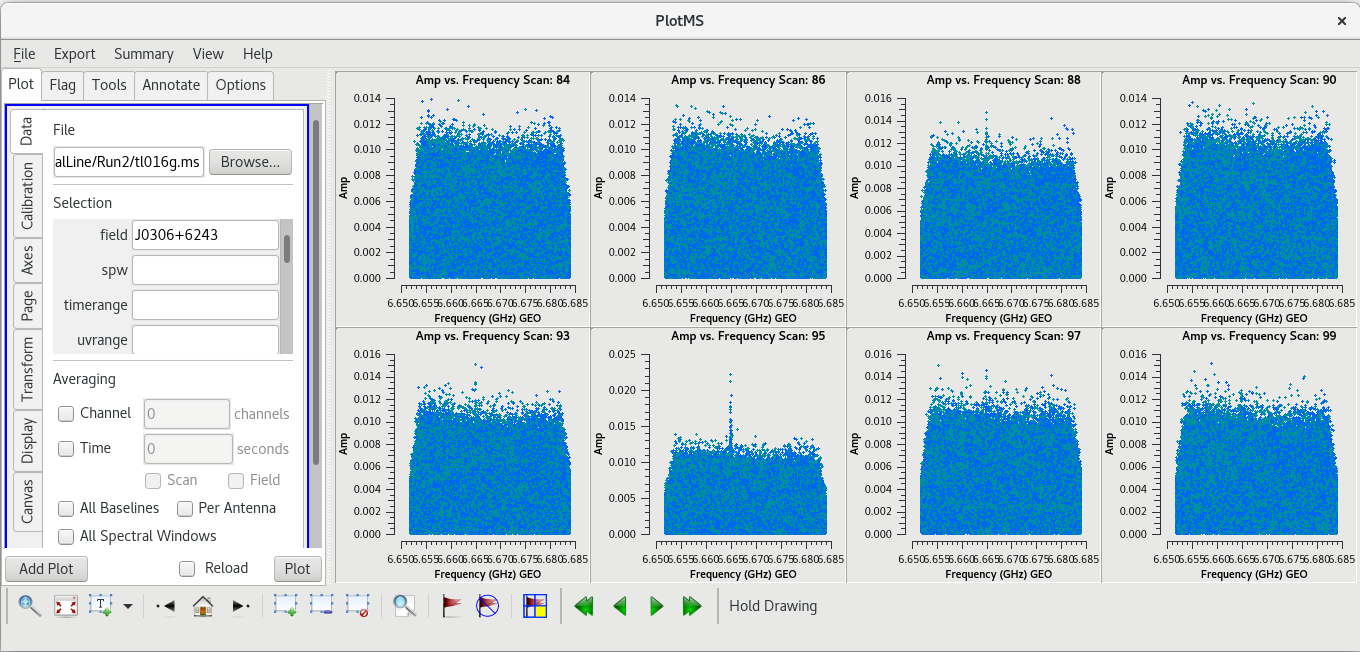
Now let's take a look at the phase reference calibrator. Again, we will plot amplitude vs frequency for all the scans. It will take a little | Now let's take a look at the phase reference calibrator. Again, we will plot amplitude vs frequency for all the scans. It will take a little longer to plot because there are so many more scans on this source. | ||
<source lang="python"> | <source lang="python"> | ||
| Line 514: | Line 514: | ||
| [[File: vlba_SpectralLine_ampvfreq_J0102_allscans.png|300px|left|thumb|Figure 18: Amplitude vs frequency for J0102+5824, all scans. These plots look pretty good, with not obvious signs of RFI.]] | | [[File: vlba_SpectralLine_ampvfreq_J0102_allscans.png|300px|left|thumb|Figure 18: Amplitude vs frequency for J0102+5824, all scans. These plots look pretty good, with not obvious signs of RFI.]] | ||
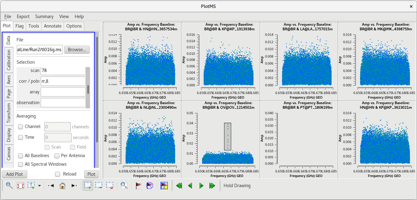
| [[File: vlba_SpectralLine_ampvfreq_J0306_scan78.png|300px|right|thumb|Figure 19: Amplitude vs frequency for several scans on J0306+6243. Notice the spike on scan 78.]] | | [[File: vlba_SpectralLine_ampvfreq_J0306_scan78.png|300px|right|thumb|Figure 19: Amplitude vs frequency for several scans on J0306+6243. Notice the spike on scan 78.]] | ||
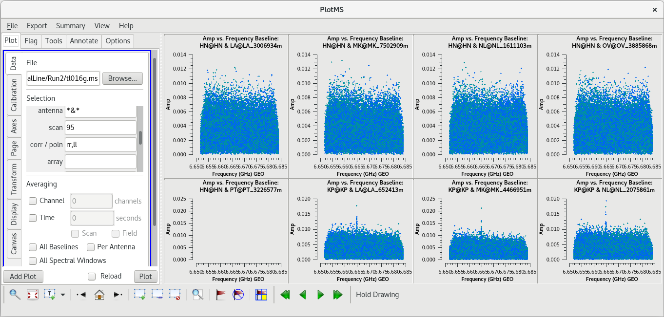
| [[File: vlba_SpectralLine_ampvfreq_J0306_scan95.png|300px|right|thumb|Figure | | [[File: vlba_SpectralLine_ampvfreq_J0306_scan95.png|300px|right|thumb|Figure 20: Amplitude vs frequency for several scans on J0306+6243. Notice the spike on scan 95.]] | ||
|} | |} | ||
| Line 531: | Line 531: | ||
</source> | </source> | ||
You can see the bad data points are all above the value 0.015. Keep in mind that this is uncalibrated data, so the units on the Y axis don't really mean anything yet. We can get rid of these bad points by using ''mode='clip''' in [https://casadocs.readthedocs.io/en/v6. | You can see the bad data points are all above the value 0.015. Keep in mind that this is uncalibrated data, so the units on the Y axis don't really mean anything yet. We can get rid of these bad points by using ''mode='clip''' in [https://casadocs.readthedocs.io/en/v6.6.5/api/tt/casatasks.flagging.flagdata.html flagdata]. | ||
<source lang="python"> | <source lang="python"> | ||
| Line 538: | Line 538: | ||
</source> | </source> | ||
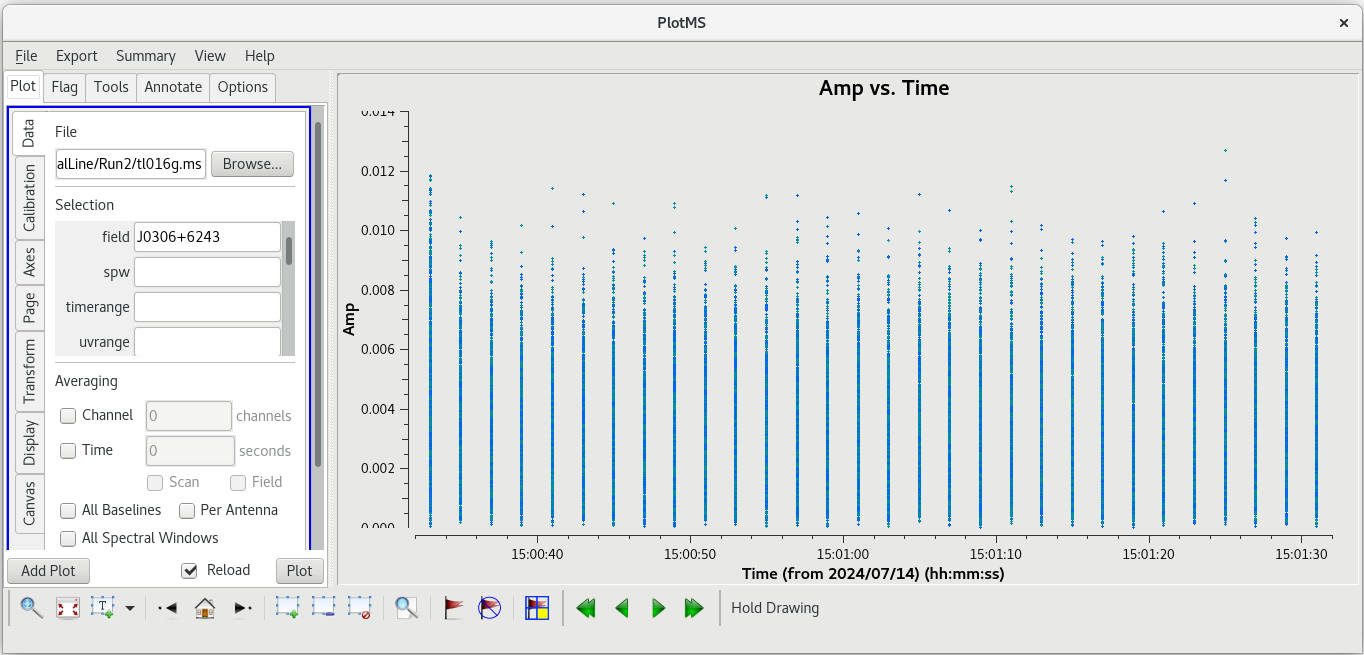
The combination of ''clipminmax=[0.0, 0.015]'' and ''clipoutside=True'' tells [https://casadocs.readthedocs.io/en/v6. | The combination of ''clipminmax=[0.0, 0.015]'' and ''clipoutside=True'' tells [https://casadocs.readthedocs.io/en/v6.6.5/api/tt/casatasks.flagging.flagdata.html flagdata] to flag anything with values outside of the range 0.0 to 0.015. If you kept the [https://casadocs.readthedocs.io/en/v6.6.5/api/tt/casaplotms.plotms.html plotms] window open, click "Reload" and the "Plot" to show the results of clipping the scan. You should see that all the bad data points are now gone, but the good data remains. | ||
{| | {| | ||
| Line 553: | Line 553: | ||
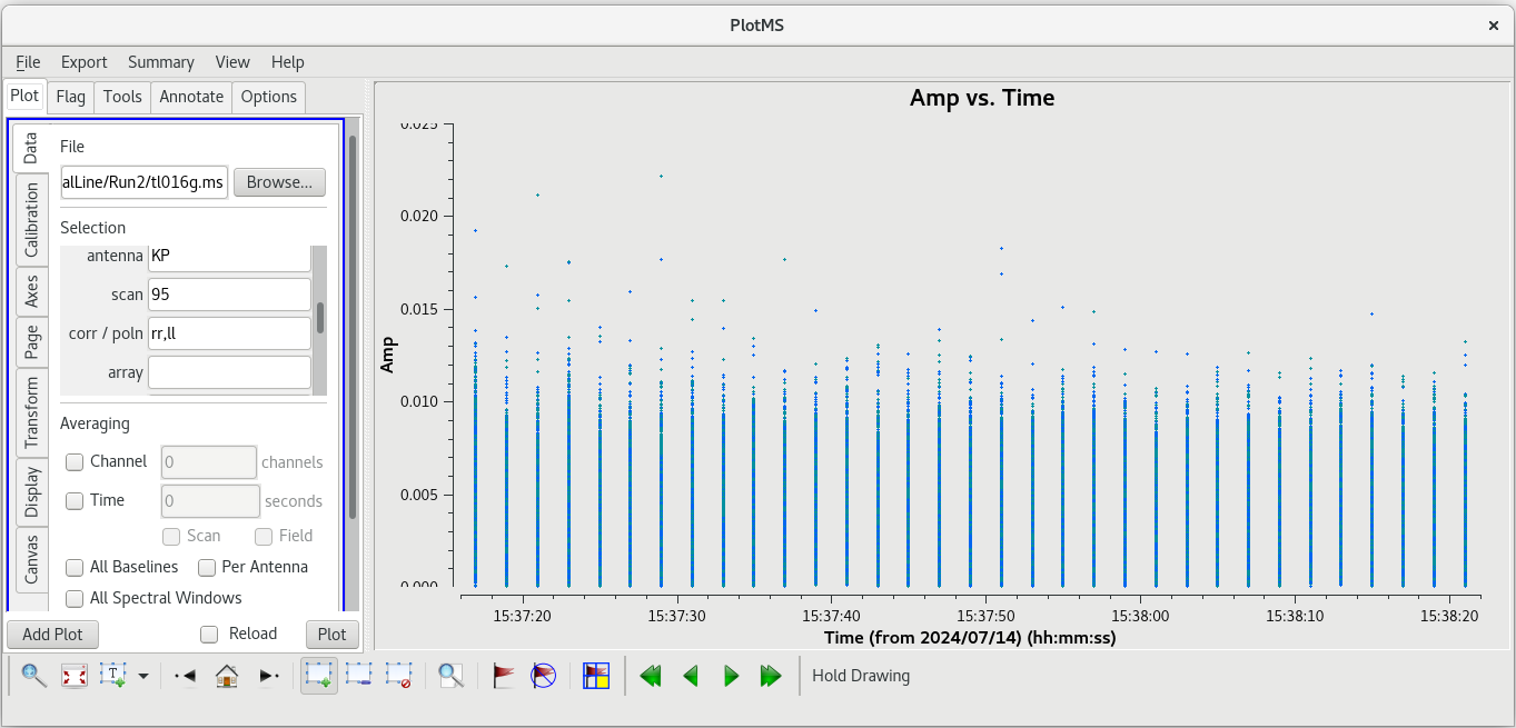
</source> | </source> | ||
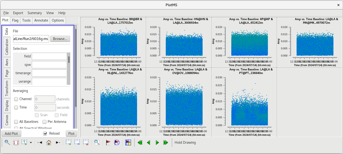
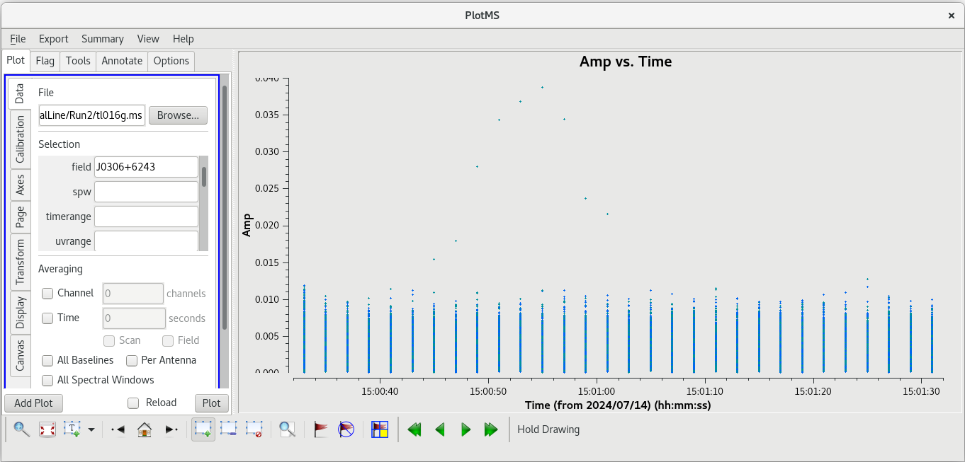
Using the GUI to step through the pages, you should notice that the spike is present on all baselines to KP. Let's take a look at | Using the GUI to step through the pages, you should notice that the spike is present on all baselines to KP. Let's take a look at amplitude vs time on KP for this scan. | ||
<source lang="python"> | <source lang="python"> | ||
| Line 561: | Line 561: | ||
{| | {| | ||
| [[File: vlba_SpectralLine_ampvfreq_scan95_baselines.png|300px|left|thumb|Figure 24: Amplitude vs frequency for scan 95, iterating on baselines. The spike is | | [[File: vlba_SpectralLine_ampvfreq_scan95_baselines.png|300px|left|thumb|Figure 24: Amplitude vs frequency for scan 95, iterating on baselines. The spike is on all baselines to KP]] | ||
| [[File: vlba_SpectralLine_ampvtime_scan95_KP.png|300px|left|thumb|Figure 25: Amplitude vs time for scan 95, all baselines to KP.]] | | [[File: vlba_SpectralLine_ampvtime_scan95_KP.png|300px|left|thumb|Figure 25: Amplitude vs time for scan 95, all baselines to KP.]] | ||
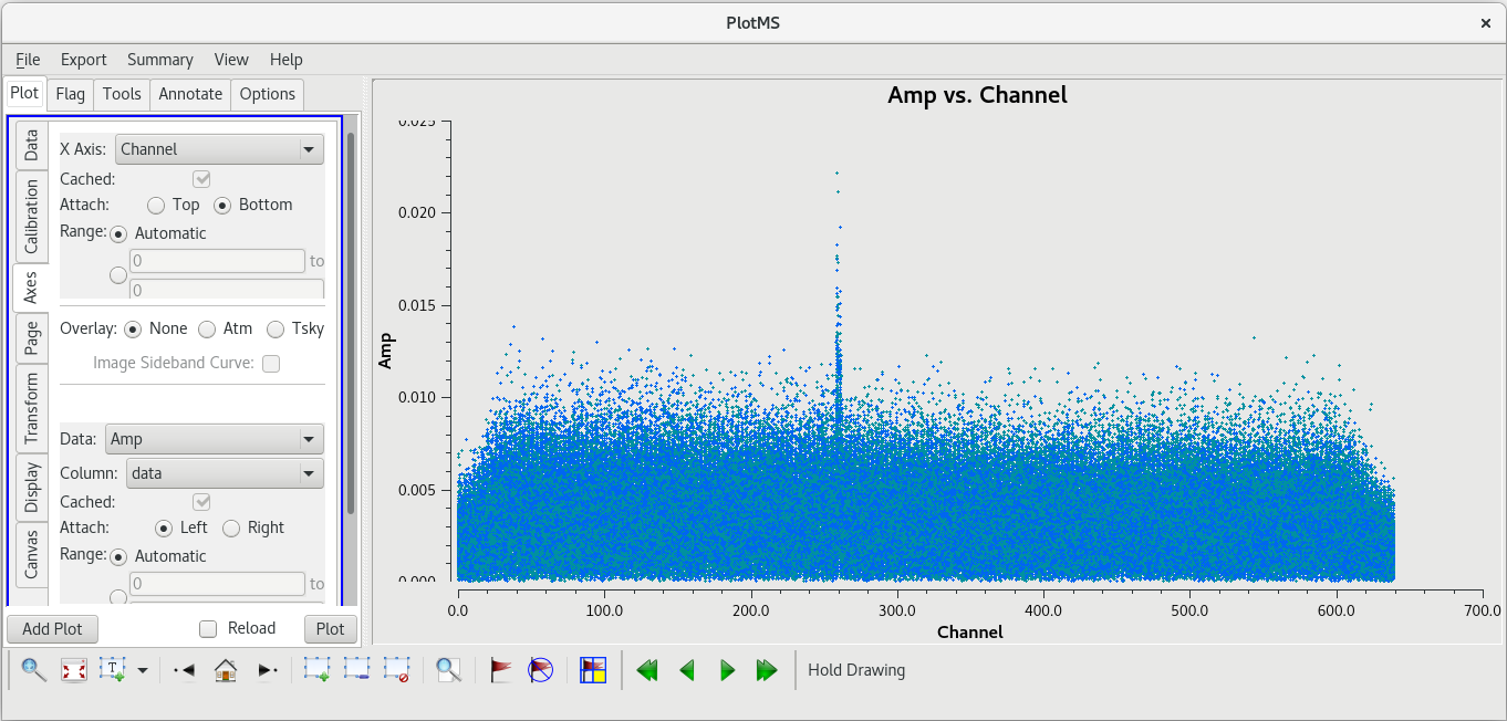
| [[File: vlba_SpectralLine_ampvchannel_scan95_KP.png|300px|right|thumb|Figure 26: Amplitude vs spectral channel for scan 95, all baselines to KP. Notice that the bad data are limited to a few spectral channels.]] | | [[File: vlba_SpectralLine_ampvchannel_scan95_KP.png|300px|right|thumb|Figure 26: Amplitude vs spectral channel for scan 95, all baselines to KP. Notice that the bad data are limited to a few spectral channels.]] | ||
| Line 568: | Line 568: | ||
|} | |} | ||
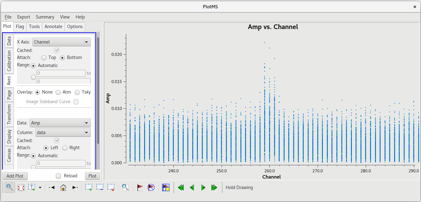
The bad data are not as obvious in this plot, and seem to cover the entire scan. If the bad data are not limited in time, they still appeared to be limited in frequency. In the GUI, go to the "Axes" tab and change the X-Axis to "Channel", then click "Plot. You should see that the bad data are indeed limited to a few spectral channels. Use the "Zoom" tool (the magnifying glass at the bottom left of the GUI) to select the region around the bad points. You should see that the bad data are limited to channels 258 to 262, so let's flag those channels on KP for this scan. To flag a select number of spectral channels, you need to use the ''spw'' parameter. In our case, set ''spw='0:258~262'''. The ''0'' is for the spectral window (we only have the one in our data), and ''258~262'' tells [https://casadocs.readthedocs.io/en/v6. | The bad data are not as obvious in this plot, and seem to cover the entire scan. If the bad data are not limited in time, they still appeared to be limited in frequency. In the GUI, go to the "Axes" tab and change the X-Axis to "Channel", then click "Plot. You should see that the bad data are indeed limited to a few spectral channels. Use the "Zoom" tool (the magnifying glass at the bottom left of the GUI) to select the region around the bad points. You should see that the bad data are limited to channels 258 to 262, so let's flag those channels on KP for this scan. To flag a select number of spectral channels, you need to use the ''spw'' parameter. In our case, set ''spw='0:258~262'''. The ''0'' is for the spectral window (we only have the one in our data), and ''258~262'' tells [https://casadocs.readthedocs.io/en/v6.6.5/api/tt/casatasks.flagging.flagdata.html flagdata] to flag all channels in the ragne 258 to 262. | ||
<source lang="python"> | <source lang="python"> | ||
| Line 575: | Line 575: | ||
</source> | </source> | ||
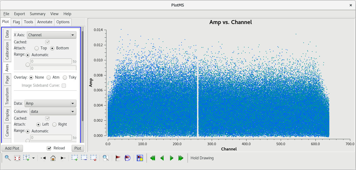
If your [https://casadocs.readthedocs.io/en/v6. | If your [https://casadocs.readthedocs.io/en/v6.6.5/api/tt/casaplotms.plotms.html plotms] window is still open, click "Reload" and "Plot" to show the impact of flagging the channels with the bad data. | ||
These are the only major issues we spotted after the automated flagging, so now we will move on to the calibration. | These are the only major issues we spotted after the automated flagging, so now we will move on to the calibration. | ||
== Calibrating the Data == | == Calibrating the Data == | ||
| Line 584: | Line 583: | ||
=== Earth Orientation Parameter Correction === | === Earth Orientation Parameter Correction === | ||
When VLBI data are correlated, the correlator uses a model for where the Earth was in its rotation. Most of the time, that model is very good and the results are perfectly fine. Sometimes, however, the model is not quite good enough (e.g., a major earthquake happened in Hawaii during the time between when the model was made and when the observation occured, and the island moved a few millimeters). In these cases, it is | When VLBI data are correlated, the correlator uses a model for where the Earth was in its rotation. Most of the time, that model is very good and the results are perfectly fine. Sometimes, however, the model is not quite good enough (e.g., a major earthquake happened in Hawaii during the time between when the model was made and when the observation occured, and the island moved a few millimeters). In these cases, it is important to make corrections for the inaccurate Earth orientation model. | ||
NASA and others host sites that contain the most up-to-date | NASA and others host sites that contain the most up-to-date Earth Orientation Parameters (EOP). You will need to retrieve the EOP from one of these hosts in order to make the EOP corrections to your data. To get the EOP file from NASA, use the curl command: | ||
curl -u anonymous:<your-email-address> --ftp-ssl ftp://gdc.cddis.eosdis.nasa.gov/vlbi/gsfc/ancillary/solve_apriori/usno_finals.erp > /<path>/<to>/<file>/usno_finals.erp | curl -u anonymous:<your-email-address> --ftp-ssl ftp://gdc.cddis.eosdis.nasa.gov/vlbi/gsfc/ancillary/solve_apriori/usno_finals.erp > /<path>/<to>/<file>/usno_finals.erp | ||
| Line 598: | Line 597: | ||
You can keep the filename as "usno_finals.erp" or change it to something that makes sense to you. For this tutorial, we assume the filename is the default "usno_finals.erp". | You can keep the filename as "usno_finals.erp" or change it to something that makes sense to you. For this tutorial, we assume the filename is the default "usno_finals.erp". | ||
Once you have the EOP file, you will create the EOP correction table using the [https://casadocs.readthedocs.io/en/v6. | Once you have the EOP file, you will create the EOP correction table using the [https://casadocs.readthedocs.io/en/v6.6.5/api/tt/casatasks.calibration.gencal.html gencal] task. | ||
<source lang="python"> | <source lang="python"> | ||
| Line 607: | Line 606: | ||
This will create the file "tl016g.eop" that contains the EOP calibration table. | This will create the file "tl016g.eop" that contains the EOP calibration table. | ||
You should check that the EOP values make sense by plotting them with [https://casadocs.readthedocs.io/en/v6. | You should check that the EOP values make sense by plotting them with [https://casadocs.readthedocs.io/en/v6.6.5/api/tt/casaplotms.plotms.html plotms]. | ||
<source lang="python"> | <source lang="python"> | ||
| Line 614: | Line 613: | ||
</source> | </source> | ||
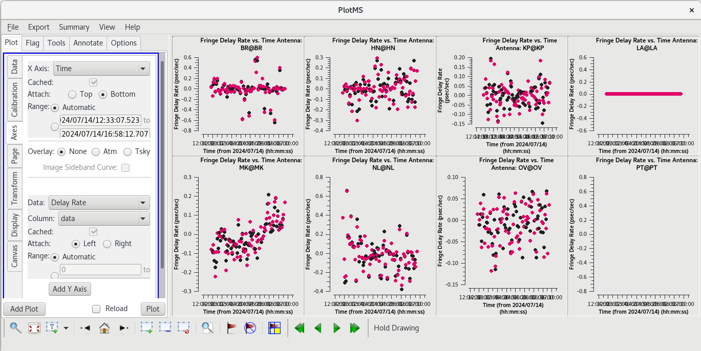
For each | For each target (field), the phases should be nice and smooth and the values should be small (about 10 degrees or less). Also check the delays and rates by going to the "Axes" tab in the GUI and changing the Y Axis to "delay" and "delay-rate", and clicking on "Plot". These should also be smooth with time and the values should be small. | ||
{| | {| | ||
| Line 626: | Line 625: | ||
=== Amplitude Corrections from Autocorrelations === | === Amplitude Corrections from Autocorrelations === | ||
Determine the amplitude corrections from the autocorrelations with [https://casadocs.readthedocs.io/en/v6. | Determine the amplitude corrections from the autocorrelations with [https://casadocs.readthedocs.io/en/v6.6.5/api/tt/casatasks.calibration.accor.html accor]. This corrects for errors introduced by the 2-bit sampling at the VLBA. | ||
<source lang="python"> | <source lang="python"> | ||
#In CASA | #In CASA | ||
accor(vis='tl016g.ms', caltable='tl016g.accor', solint='30s') | accor(vis='tl016g.ms', caltable='tl016g.accor', solint='30s', gaintable=['tl016g.eop'], interp=['nearest']) | ||
</source> | </source> | ||
<b>NOTE:</b> This step is not required for EVN data, because the EVN correlator performs it during correlation. | <b>NOTE:</b> This step is not required for EVN data, because the EVN correlator performs it during correlation. | ||
Inspect the tl016g.accor solution table with [https://casadocs.readthedocs.io/en/v6. | Inspect the tl016g.accor solution table with [https://casadocs.readthedocs.io/en/v6.6.5/api/tt/casaplotms.plotms.html plotms]. | ||
<source lang="python"> | <source lang="python"> | ||
#In CASA | #In CASA | ||
| Line 644: | Line 643: | ||
Ideally, all of the solutions should be very close to 1.0. Looking through the solutions, you can see that everything is close to 1, but the solutions look a bit noisy. | Ideally, all of the solutions should be very close to 1.0. Looking through the solutions, you can see that everything is close to 1, but the solutions look a bit noisy. | ||
The AIPS VLBA utility script VLBACCOR smooths the autocorrelation corrections by default (with a smoothing time of 30 minutes). It is possible to do this smoothing in CASA 6.3 and later using the [https://casadocs.readthedocs.io/en/v6. | The AIPS VLBA utility script VLBACCOR smooths the autocorrelation corrections by default (with a smoothing time of 30 minutes). It is possible to do this smoothing in CASA 6.3 and later using the [https://casadocs.readthedocs.io/en/v6.6.5/api/tt/casatasks.calibration.smoothcal.html smoothcal] task. Based on what we saw in our plotting, these data would likely benefit from some smoothing. | ||
<source lang="python"> | <source lang="python"> | ||
#In CASA | #In CASA | ||
smoothcal(vis='tl016g.ms', tablein=' | smoothcal(vis='tl016g.ms', tablein='tl016bg.accor', caltable='tl016g_smooth.accor', smoothtype='median', smoothtime=1800.0) | ||
</source> | </source> | ||
Remember to check the smoothed solutions with [https://casadocs.readthedocs.io/en/v6. | Remember to check the smoothed solutions with [https://casadocs.readthedocs.io/en/v6.6.5/api/tt/casaplotms.plotms.html plotms] to make sure it was an improvement. | ||
<source lang="python"> | <source lang="python"> | ||
#In CASA | #In CASA | ||
| Line 666: | Line 665: | ||
[[File:vlba_SpectralLine_Tsys.png|300px|right|thumb|Figure 34: Plot of system temperature vs. time. Data for each antenna is plotted separately. Notice the scale for PT is much higher than the other antennas.]] | [[File:vlba_SpectralLine_Tsys.png|300px|right|thumb|Figure 34: Plot of system temperature vs. time. Data for each antenna is plotted separately. Notice the scale for PT is much higher than the other antennas.]] | ||
Unlike the VLA, the VLBA cannot rely on bootstrapping absolute flux density calibration from a well-modeled calibrator. Instead, the VLBA relies on a combination of the system temperature and the known gain curve of the antennas (how the gain of the antenna changes with elevation). Both the system temperatures and gain curves are included in the FITS-IDI file, and both are imported into the Measurement Set with [https://casadocs.readthedocs.io/en/v6. | Unlike the VLA, the VLBA cannot rely on bootstrapping absolute flux density calibration from a well-modeled calibrator. Instead, the VLBA relies on a combination of the system temperature and the known gain curve of the antennas (how the gain of the antenna changes with elevation). Both the system temperatures and gain curves are included in the FITS-IDI file, and both are imported into the Measurement Set with [https://casadocs.readthedocs.io/en/v6.6.5/api/tt/casatasks.data.importfitsidi.html importfitsidi]. To get the system temperature and gain curve information into a form that CASA can use for calibration, we use the [https://casadocs.readthedocs.io/en/v6.6.5/api/tt/casatasks.calibration.gencal.html gencal] task to generate calibration tables. | ||
<b>System temperature:</b> | <b>System temperature:</b> | ||
| Line 673: | Line 672: | ||
</source> | </source> | ||
Check the system temperature table with [https://casadocs.readthedocs.io/en/v6. | Check the system temperature table with [https://casadocs.readthedocs.io/en/v6.6.5/api/tt/casaplotms.plotms.html plotms]. | ||
<source lang="python"> | <source lang="python"> | ||
#In CASA | #In CASA | ||
| Line 679: | Line 678: | ||
</source> | </source> | ||
The system temperature values mostly look good. They vary smoothly at most stations, and the values are reasonable for C-band (between about 20 and 50 K). Notice that you cannot really tell the difference between scans on maser and scans on calibrators. Even though the maser lines are | The system temperature values mostly look good. They vary smoothly at most stations, and the values are reasonable for C-band (between about 20 and 50 K). Notice that you cannot really tell the difference between scans on maser and scans on calibrators. Even though the maser lines are incredibly bright, they are so narrow that they do not impact the system temperatures much. There is some weird behavior on NL during the earliest scans, but the values are not too high. There are major problems on PT, however. That broadband RFI that we noticed earlier caused the system temperature values for that station to be very high and messy. If we had not already flagged the PT antenna, we would definitely do it now. | ||
<b>Gain curve:</b> | <b>Gain curve:</b> | ||
| Line 686: | Line 685: | ||
gencal(vis='tl016g.ms', caltable='tl016g.gcal', caltype='gc') | gencal(vis='tl016g.ms', caltable='tl016g.gcal', caltype='gc') | ||
</source> | </source> | ||
This observation was done at 6.7 GHz and with a bandwidth of only 32 MHz. The gain curve is very uninteresting, so we will not bother looking at the solutions now (although you can if you really want to). If your observation is at 12 GHz or higher, you will probably want to inspect the gain curve table with [https://casadocs.readthedocs.io/en/v6. | This observation was done at 6.7 GHz and with a bandwidth of only 32 MHz. The gain curve is very uninteresting, so we will not bother looking at the solutions now (although you can if you really want to). If your observation is at 12 GHz or higher, you will probably want to inspect the gain curve table with [https://casadocs.readthedocs.io/en/v6.6.5/api/tt/casaplotms.plotms.html plotms]. | ||
<b>NOTE: </b> For EVN observations, the system temperatures and gain curves are provided in ANTAB files rather than in the FITS-IDI file. If you are working with EVN data, you must append the system temperature data to the FITS-IDI file before running [https://casadocs.readthedocs.io/en/v6. | <b>NOTE: </b> For EVN observations, the system temperatures and gain curves are provided in ANTAB files rather than in the FITS-IDI file. If you are working with EVN data, you must append the system temperature data to the FITS-IDI file before running [https://casadocs.readthedocs.io/en/v6.6.5/api/tt/casatasks.data.importfitsidi.html importfitsidi]. EVN gain curves must also be extracted from the ANTAB file. For more information, see the [https://www.evlbi.org/evn-data-reduction-guide EVN Data Reduction Guide]. | ||
=== Instrumental Delay Calibration === | === Instrumental Delay Calibration === | ||
Solve for the instrumental delays by using [https://casadocs.readthedocs.io/en/v6. | Solve for the instrumental delays by using [https://casadocs.readthedocs.io/en/v6.6.5/api/tt/casatasks.calibration.fringefit.html fringefit] on a bright source (the "fringe finder"). In our case, the fringe finder is J0102+5824. Set the ''timerange'' to the one-minute time span you identified while inspecting the data earlier. Because we are only solving for the instrumental delays (changes in phase as a function of frequency), we will set ''zerorates=True'' to set all of the delay-rates (changes in phase as a function of time) to be zero. | ||
<source lang="python"> | <source lang="python"> | ||
#In CASA | #In CASA | ||
| Line 698: | Line 697: | ||
</source> | </source> | ||
Notice that we are pre-applying the EOP, sampling corrections, gain curve, and system temperature when we run [https://casadocs.readthedocs.io/en/v6. | Notice that we are pre-applying the EOP, sampling corrections, gain curve, and system temperature when we run [https://casadocs.readthedocs.io/en/v6.6.5/api/tt/casatasks.calibration.fringefit.html fringefit]. We are also applying the parallactic angle correction (''parang=True''), which is necessary to do prior to any phase referencing. | ||
Watch the logger for any reports of low SNR and failures to converge on a solution. Ideally, the SNR for each station should be very high (for our data, all reported SNR values are larger than 380, which is pretty good). | Watch the logger for any reports of low SNR and failures to converge on a solution. Ideally, the SNR for each station should be very high (for our data, all reported SNR values are larger than 380, which is pretty good). | ||
<b>A Note on Table Names:</b> In the Basic Phase-referencing tutorial, we followed the convention of naming tables as described in the EVN CASA tutorials. The instrumental delay table was called "sbd", which stood for "single band delay". It is not necessary to follow this convention. You can name a calibration table anything you want. For example, | <b>A Note on Table Names:</b> In the Basic Phase-referencing tutorial, we followed the convention of naming tables as described in the EVN CASA tutorials. The instrumental delay table was called "sbd", which stood for "single band delay". It is not necessary to follow this convention. You can name a calibration table anything you want. For example, you could set ''caltable='tl106g.instdly''' for the instrumental delay. Just be sure to keep track of your tables and to apply them appropriately in the calibration tasks. | ||
Once [https://casadocs.readthedocs.io/en/v6. | Once [https://casadocs.readthedocs.io/en/v6.6.5/api/tt/casatasks.calibration.fringefit.html fringefit] has finished, you should see the following in the logger: | ||
<pre style="background-color: #fffacd;"> | <pre style="background-color: #fffacd;"> | ||
Finished solving. | Finished solving. | ||
| Line 712: | Line 711: | ||
This is exactly what we expect to see. We are only attempting to get one solution per spw because we are only solving over a single solution interval (one minute of data from a single scan). | This is exactly what we expect to see. We are only attempting to get one solution per spw because we are only solving over a single solution interval (one minute of data from a single scan). | ||
Apply the instrumental delay corrections using [https://casadocs.readthedocs.io/en/v6. | Apply the instrumental delay corrections using [https://casadocs.readthedocs.io/en/v6.6.5/api/tt/casatasks.calibration.applycal.html applycal]. | ||
<source lang="python"> | <source lang="python"> | ||
| Line 718: | Line 717: | ||
applycal(vis='tl016g.ms', gaintable=['tl016g.eop', 'tl016g_smooth.accor', 'tl016g.gcal', 'tl016g.tsys', 'tl016g.sbd'], interp=['nearest', 'nearest', 'nearest', 'nearest,nearest', 'nearest'], parang=True) | applycal(vis='tl016g.ms', gaintable=['tl016g.eop', 'tl016g_smooth.accor', 'tl016g.gcal', 'tl016g.tsys', 'tl016g.sbd'], interp=['nearest', 'nearest', 'nearest', 'nearest,nearest', 'nearest'], parang=True) | ||
</source> | </source> | ||
<b>NOTE:</b> In [https://casadocs.readthedocs.io/en/v6. | <b>NOTE:</b> In [https://casadocs.readthedocs.io/en/v6.6.5/api/tt/casatasks.calibration.applycal.html applycal], the order in which you specify the list for ''gaintable'' sets the order for both ''interp'' and ''spwmap''. If you change the order of ''gaintable'', be sure to also change the order of ''interp'' and ''spwmap''! Also, if you smoothed any of the solutions, be sure to use the appropriate filename for the smoothed table. | ||
It may take a little while (~2 minutes or more) for [https://casadocs.readthedocs.io/en/v6. | It may take a little while (~2 minutes or more) for [https://casadocs.readthedocs.io/en/v6.6.5/api/tt/casatasks.calibration.applycal.html applycal] to finish. If you are watching the logger carefully, you will see the message "Adding CORRECTED_DATA column(s)". Because this is the first time that we have run [https://casadocs.readthedocs.io/en/v6.6.5/api/tt/casatasks.calibration.applycal.html applycal], CASA needs to create a new column containing the data with the corrections applied. | ||
Check that applying the solutions resulted in improvements: | Check that applying the solutions resulted in improvements: | ||
| Line 728: | Line 727: | ||
</source> | </source> | ||
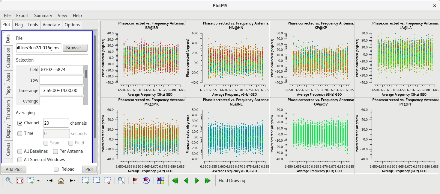
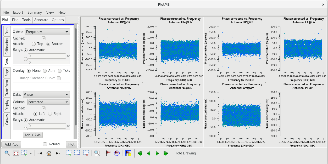
Ideally, | Ideally, the phase values should now be clustered around 0 degrees. For our data, all of the plots are nicely centered on 0 degrees, but there is a lot of scatter because of the large number of spectral channels. To make things a little easier to look at, we will average 20 spectral channels like we did when we were looking for a good reference antenna (in the "Data" tab, under "Averaging", check the box next to "Channels" and change the value to 20, then click "Plot"). The averaged plots should have much less scatter in the phases. | ||
| Line 738: | Line 737: | ||
=== Global Fringe Fitting === | === Global Fringe Fitting === | ||
Now, we will solve for the time and frequency-dependent effects in phase using [https://casadocs.readthedocs.io/en/v6. | Now, we will solve for the time and frequency-dependent effects in phase using [https://casadocs.readthedocs.io/en/v6.6.5/api/tt/casatasks.calibration.fringefit.html fringefit], also known as "global fringe fitting" (or sometimes "multi-band delay", if you have multiple spectral windows and you combine them during this step). We will need to pick a solution interval that is appropriate for our data. It should be at least 10 seconds, and no longer than the scan length on the phase reference calibrator. For this observation, we will need to use ''solint='inf''', which will give one solution for each scan on the calibrator sources. | ||
<b>NOTE: </b>You are welcome to try a shorter solution interval, but you will probably run into a problem where there is a tiny bit of a scan | <b>NOTE: </b>You are welcome to try a shorter solution interval, but you will probably run into a problem where there is a tiny bit of a scan left after the solution interval and [https://casadocs.readthedocs.io/en/v6.6.5/api/tt/casatasks.calibration.fringefit.html fringefit] will fail. | ||
For ''refant'', enter a list of antennas to try as the reference antenna. The preferred ''refant'' should be listed first, followed by the second choice, then third choice, and so on. It is not recommended to include Mauna Kea (MK) or Saint Croix (SC) in the list, unless the phase reference calibrator is very bright on the longest baselines. BR and HN are often omitted for the same reason. For our observation, we will set the list to LA, KP, OV, and NL. Set ''field'' to the fringe finder, the backup fringe finder, and the phase reference calibrator. | For ''refant'', enter a list of antennas to try as the reference antenna. The preferred ''refant'' should be listed first, followed by the second choice, then third choice, and so on. It is not recommended to include Mauna Kea (MK) or Saint Croix (SC) in the list, unless the phase reference calibrator is very bright on the longest baselines. BR and HN are often omitted for the same reason. For our observation, we will set the list to LA, KP, OV, and NL. Set ''field'' to the fringe finder, the backup fringe finder, and the phase reference calibrator. | ||
| Line 751: | Line 750: | ||
This step may take quite a while (probably at least 20 minutes), so this is a good opportunity to stand up, stretch, and go get a tasty beverage. | This step may take quite a while (probably at least 20 minutes), so this is a good opportunity to stand up, stretch, and go get a tasty beverage. | ||
When the [https://casadocs.readthedocs.io/en/v6. | When the [https://casadocs.readthedocs.io/en/v6.6.5/api/tt/casatasks.calibration.fringefit.html fringefit] task is done, check the logger for the solution statistics ("expected/attempted/succeeded"). You want all three numbers to be the same, or at least very similar. | ||
For our project, you should see something like this in the logger: | For our project, you should see something like this in the logger: | ||
| Line 760: | Line 759: | ||
</pre> | </pre> | ||
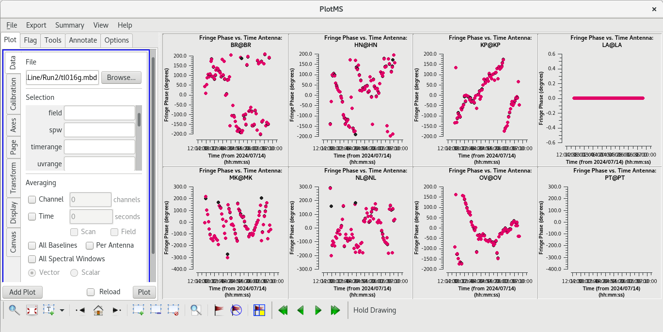
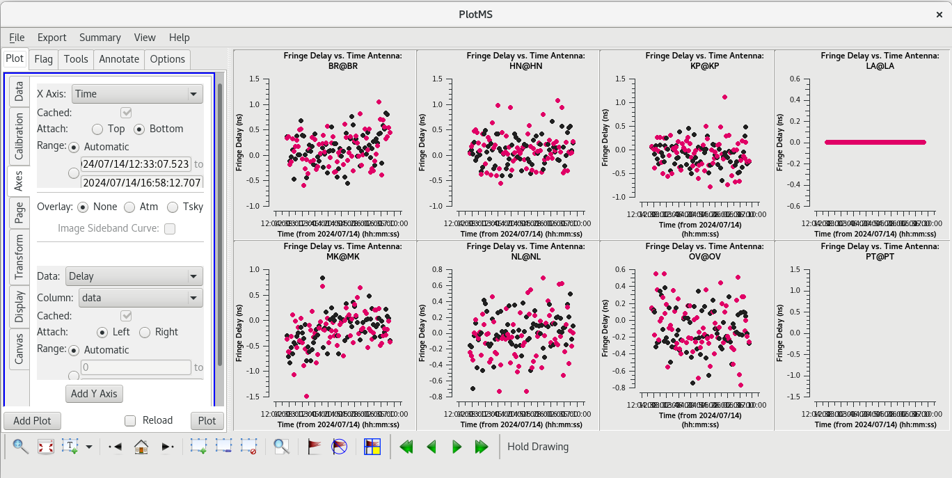
Because [https://casadocs.readthedocs.io/en/v6. | Because [https://casadocs.readthedocs.io/en/v6.6.5/api/tt/casatasks.calibration.fringefit.html fringefit] ran successfully and we are satisfied that the number of solutions is appropriate, we should now take a look at the solutions with [https://casadocs.readthedocs.io/en/v6.6.5/api/tt/casaplotms.plotms.html plotms]. | ||
<source lang="python"> | <source lang="python"> | ||
| Line 775: | Line 774: | ||
Use the GUI to switch the ''yaxis'' between 'Phase', 'Delay', and 'Delay Rate'. The phase and delay solutions should both vary smoothly with time. If they do not, you may need to smooth the table before applying it. The delay-rates should be clustered around zero with some scatter. You should see that the solutions on all antennas look pretty good. | Use the GUI to switch the ''yaxis'' between 'Phase', 'Delay', and 'Delay Rate'. The phase and delay solutions should both vary smoothly with time. If they do not, you may need to smooth the table before applying it. The delay-rates should be clustered around zero with some scatter. You should see that the solutions on all antennas look pretty good. | ||
Now that we are confident that the global [https://casadocs.readthedocs.io/en/v6. | Now that we are confident that the global [https://casadocs.readthedocs.io/en/v6.6.5/api/tt/casatasks.calibration.fringefit.html fringefit] solutions are good, we will apply them with [https://casadocs.readthedocs.io/en/v6.6.5/api/tt/casatasks.calibration.applycal.html applycal]. | ||
<source lang="python"> | <source lang="python"> | ||
#In CASA | #In CASA | ||
applycal(vis='tl016g.ms', gaintable=['tl016g.eop', 'tl016g_smooth.accor', 'tl016g.gcal', 'tl016g.tsys', 'tl016g.sbd', 'tl016g.mbd'], interp=['nearest', 'nearest', 'nearest', 'nearest,nearest', 'nearest', 'linear'], parang=True) | applycal(vis='tl016g.ms', gaintable=['tl016g.eop', 'tl016g_smooth.accor', 'tl016g.gcal', 'tl016g.tsys', 'tl016g.sbd', 'tl016g.mbd'], interp=['nearest', 'nearest', 'nearest', 'nearest,nearest', 'nearest', 'linear'], parang=True) | ||
</source> | </source> | ||
It will probably take a while (about 2 minutes) for [https://casadocs.readthedocs.io/en/v6. | It will probably take a while (about 2 minutes) for [https://casadocs.readthedocs.io/en/v6.6.5/api/tt/casatasks.calibration.applycal.html applycal] to run this time. | ||
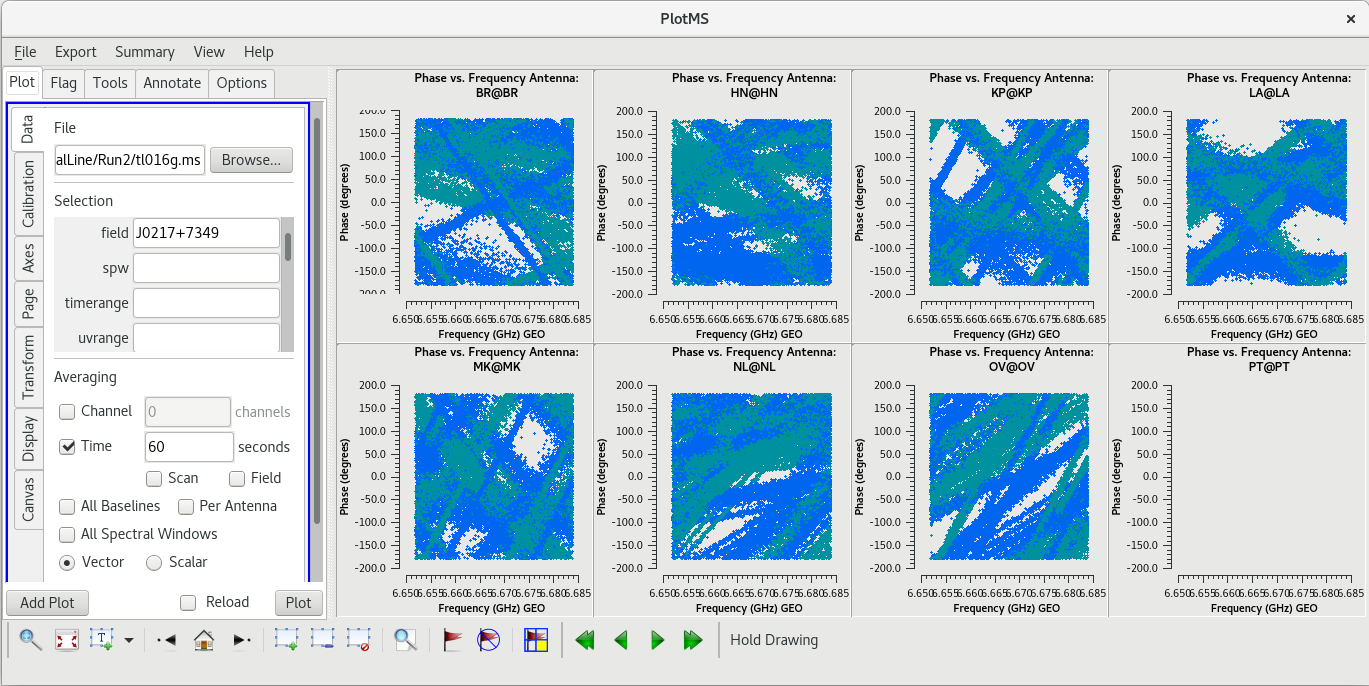
Take a look at the data with [https://casadocs.readthedocs.io/en/v6. | Take a look at the data with [https://casadocs.readthedocs.io/en/v6.6.5/api/tt/casaplotms.plotms.html plotms] to make sure the corrections are improving the phases. We'll look at the back up fringe finder, J0217+7349. We'll start by looking at the uncalibrated phases. We will average the data in the time dimension, using a 60-second average time, to be able to see the details. | ||
<source lang="python"> | <source lang="python"> | ||
| Line 799: | Line 798: | ||
=== Bandpass Calibration === | === Bandpass Calibration === | ||
Now we will correct for the shape of the bandpass using the [https://casadocs.readthedocs.io/en/v6. | Now we will correct for the shape of the bandpass using the [https://casadocs.readthedocs.io/en/v6.6.5/api/tt/casatasks.calibration.bandpass.html bandpass] task. This step requires a very bright source (perferably >1 Jy on all baselines), so we will use our fringe finder J0102+5824. However, unlike when we solved for the instrumental delay (above), we will use all of the scans on the source. | ||
<source lang="python"> | <source lang="python"> | ||
| Line 806: | Line 805: | ||
</source> | </source> | ||
Inspect the solutions with [https://casadocs.readthedocs.io/en/v6. | Inspect the solutions with [https://casadocs.readthedocs.io/en/v6.6.5/api/tt/casaplotms.plotms.html plotms]. | ||
<source lang="python"> | <source lang="python"> | ||
#In CASA | #In CASA | ||
| Line 819: | Line 818: | ||
|} | |} | ||
Apply the solutions with [https://casadocs.readthedocs.io/en/v6. | Apply the solutions with [https://casadocs.readthedocs.io/en/v6.6.5/api/tt/casatasks.calibration.applycal.html applycal]. | ||
<source lang="python"> | <source lang="python"> | ||
#In CASA | #In CASA | ||
applycal(vis='tl016g.ms', gaintable=['tl016g.eop', 'tl016g_smooth.accor', 'tl016g.gcal', 'tl016g.tsys', 'tl016g.sbd', 'tl016g.mbd', 'tl016g.bpass'], interp=['nearest', 'nearest', 'nearest', 'nearest,nearest', 'nearest', 'linear', 'linear,linear'], parang=True) | applycal(vis='tl016g.ms', gaintable=['tl016g.eop', 'tl016g_smooth.accor', 'tl016g.gcal', 'tl016g.tsys', 'tl016g.sbd', 'tl016g.mbd', 'tl016g.bpass'], interp=['nearest', 'nearest', 'nearest', 'nearest,nearest', 'nearest', 'linear', 'linear,linear'], parang=True) | ||
</source> | </source> | ||
It will probably take a while for [https://casadocs.readthedocs.io/en/v6. | It will probably take a while for [https://casadocs.readthedocs.io/en/v6.6.5/api/tt/casatasks.calibration.applycal.html applycal] to run again, since you are also applying the solutions from the global fringe fitting. | ||
After applying the bandpass solutions, take a look at the calibrated data with [https://casadocs.readthedocs.io/en/v6. | After applying the bandpass solutions, take a look at the calibrated data with [https://casadocs.readthedocs.io/en/v6.6.5/api/tt/casaplotms.plotms.html plotms]. | ||
<source lang="python"> | <source lang="python"> | ||
#In CASA | #In CASA | ||
plotms(vis='tl016g.ms', xaxis='frequency', yaxis='amp', ydatacolumn='corrected', field='J0102+5824', antenna='*&*', correlation='rr,ll', iteraxis='baseline', coloraxis='corr') | plotms(vis='tl016g.ms', xaxis='frequency', yaxis='amp', ydatacolumn='corrected', field='J0102+5824', antenna='*&*', correlation='rr,ll', gridrows=2, gridcols=4, iteraxis='baseline', coloraxis='corr') | ||
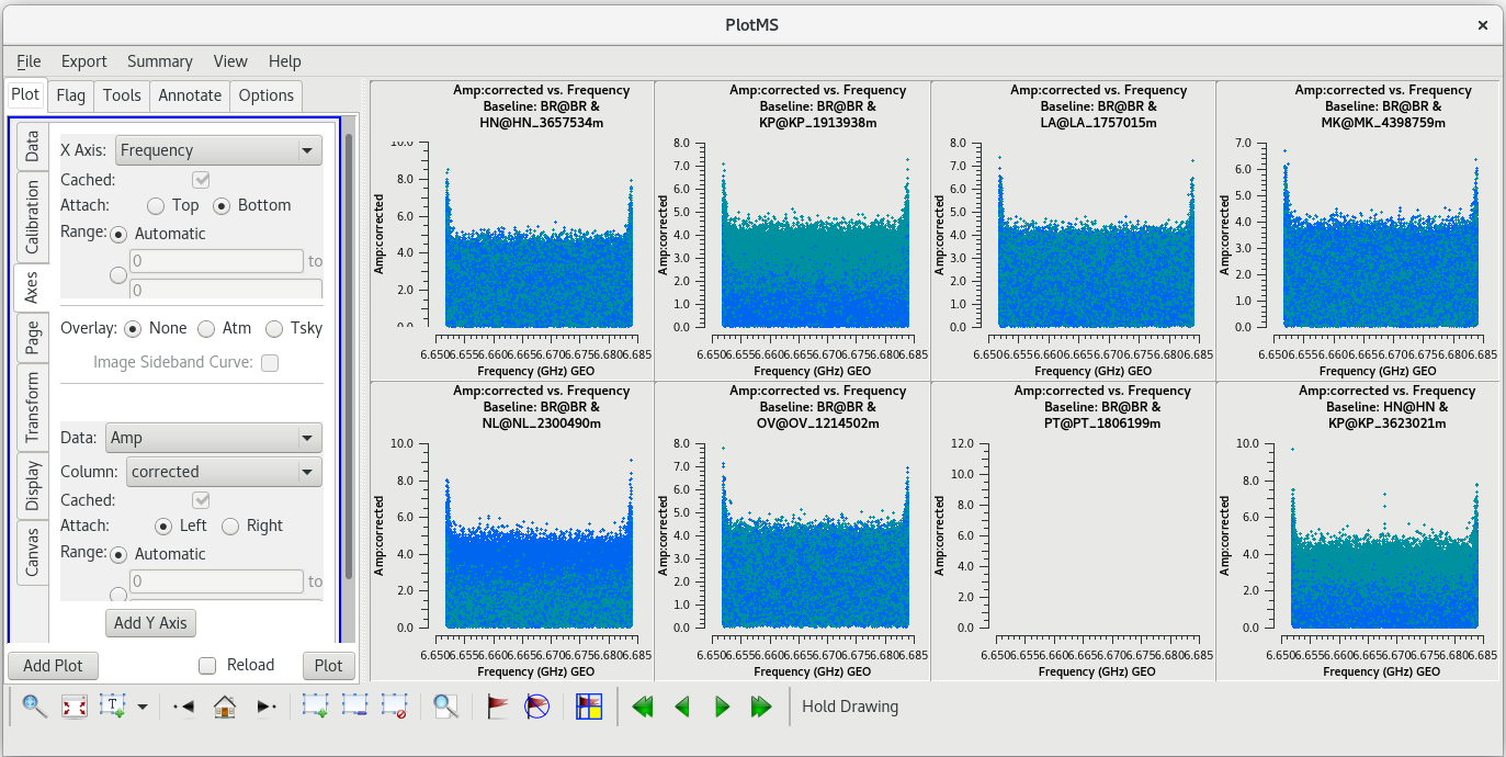
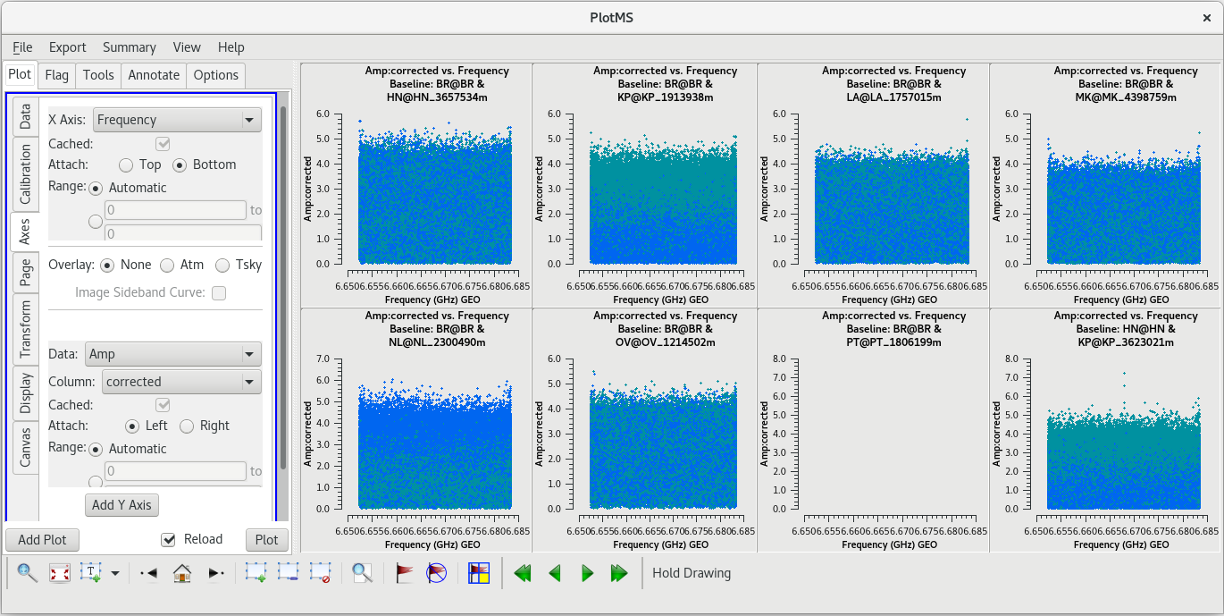
</source> | </source> | ||
| Line 838: | Line 837: | ||
</source> | </source> | ||
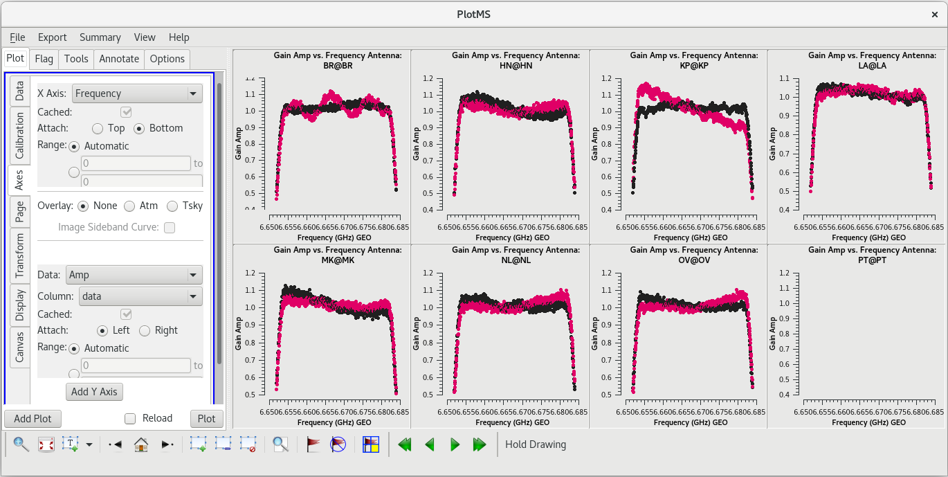
If you kep your [https://casadocs.readthedocs.io/en/v6. | If you kep your [https://casadocs.readthedocs.io/en/v6.6.5/api/tt/casaplotms.plotms.html plotms] window open, check the "Reload" box and click "Plot" to show the effect of flagging the edge channels. You should see that all of the antennas show a nice, flat bandpass. | ||
{| | {| | ||
| Line 849: | Line 848: | ||
Also, in the Basic Phase-referencing tutorial, we split the calibrated data at this point and performed self-calibration on the split file. For this tutorial, we will continue with self-calibration using the orignal data MS. The reason for this will become obvious soon. (Students are encouraged to think about why that might be and see if they are correct later!) | Also, in the Basic Phase-referencing tutorial, we split the calibrated data at this point and performed self-calibration on the split file. For this tutorial, we will continue with self-calibration using the orignal data MS. The reason for this will become obvious soon. (Students are encouraged to think about why that might be and see if they are correct later!) | ||
However, we will use [https://casadocs.readthedocs.io/en/v6. | However, we will use [https://casadocs.readthedocs.io/en/v6.6.5/api/tt/casatasks.manipulation.split.html split] to save our progress, just in case we make any mistakes after this point. | ||
<b>NOTE: </b>The split step is optional, and just a precaution in case we ake mistakes later. This will create a new 4 GB MS file on your disk. If you are very low on disk space, you may want to skip this step, or set the ''outputvis'' parameter such that it writes the new MS to an external drive. | <b>NOTE: </b>The split step is optional, and just a precaution in case we ake mistakes later. This will create a new 4 GB MS file on your disk. If you are very low on disk space, you may want to skip this step, or set the ''outputvis'' parameter such that it writes the new MS to an external drive. | ||
| Line 858: | Line 857: | ||
</source> | </source> | ||
Notice that we are not bothering to save the autocorrelations (we do not need them anymore after running [https://casadocs.readthedocs.io/en/v6. | Notice that we are not bothering to save the autocorrelations (we do not need them anymore after running [https://casadocs.readthedocs.io/en/v6.6.5/api/tt/casatasks.calibration.accor.html accor]). Setting ''datacolumn='all''' makes sure we keep both the uncalibrated data and the calibrated data. | ||
We are now done with the initial calibration. | We are now done with the initial calibration. | ||
| Line 872: | Line 871: | ||
=== Imaging the Phase Reference Calibrator === | === Imaging the Phase Reference Calibrator === | ||
To create images of our sources, we will use [https://casadocs.readthedocs.io/en/v6. | To create images of our sources, we will use [https://casadocs.readthedocs.io/en/v6.6.5/api/tt/casatasks.imaging.tclean.html tclean]. | ||
<source lang="python"> | <source lang="python"> | ||
| Line 880: | Line 879: | ||
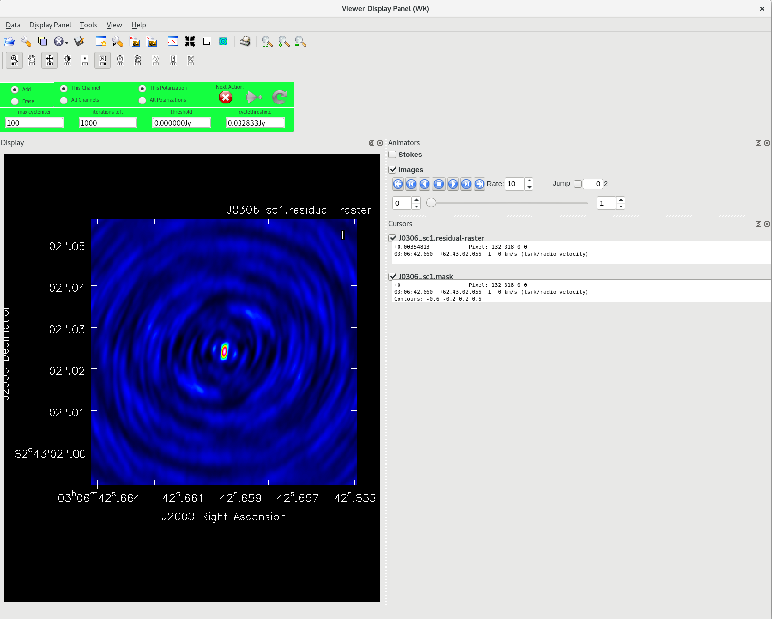
Setting ''interactive=True'' will allow us to define the areas where there is real flux from the source ("clean windows"). The value for ''niter'' needs to be large enough that we can go through enough clean iterations to recover most of the source flux. You can set ''niter'' to any arbitrarily large number (a few hundred should be plenty), but 1000 is an easy value to remember. Setting ''savemodel='modelcolumn' '' will save the model we create for the image to the model column of the measurement set so we can use it for self-calibration. | Setting ''interactive=True'' will allow us to define the areas where there is real flux from the source ("clean windows"). The value for ''niter'' needs to be large enough that we can go through enough clean iterations to recover most of the source flux. You can set ''niter'' to any arbitrarily large number (a few hundred should be plenty), but 1000 is an easy value to remember. Setting ''savemodel='modelcolumn' '' will save the model we create for the image to the model column of the measurement set so we can use it for self-calibration. | ||
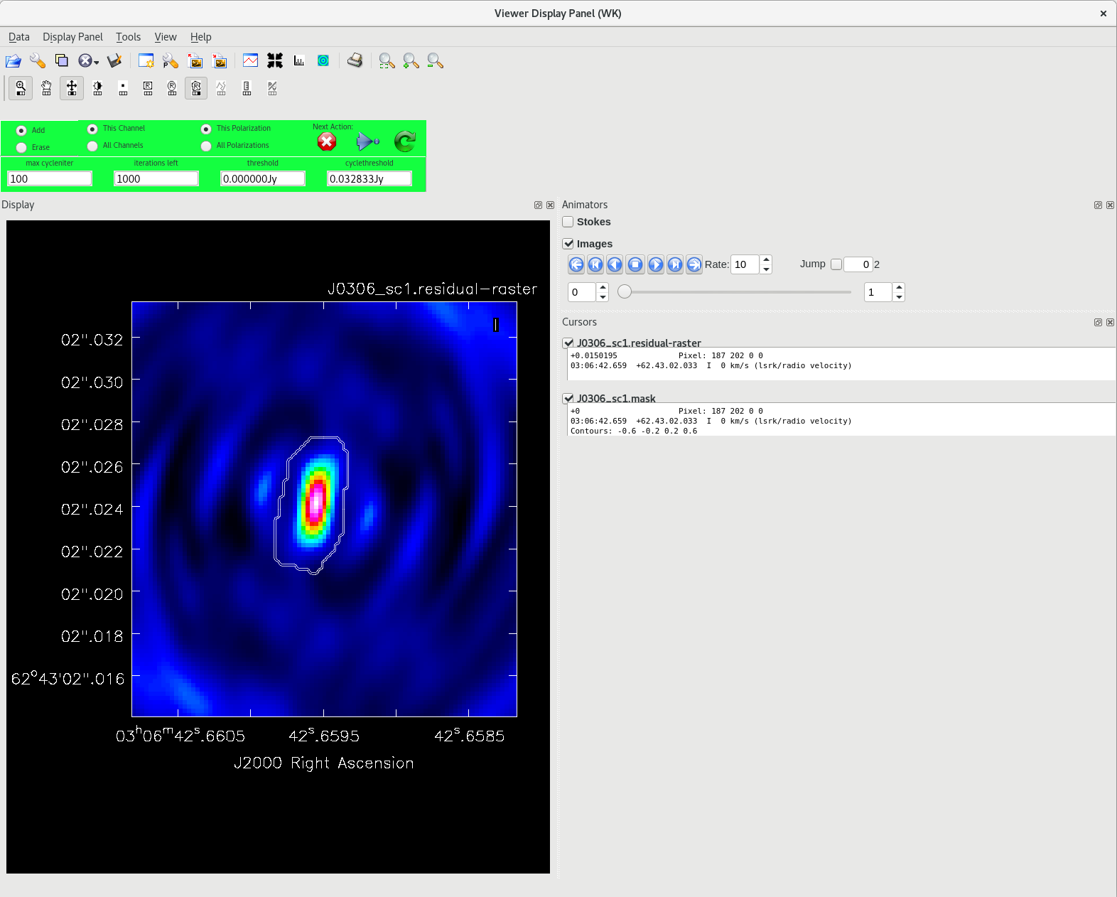
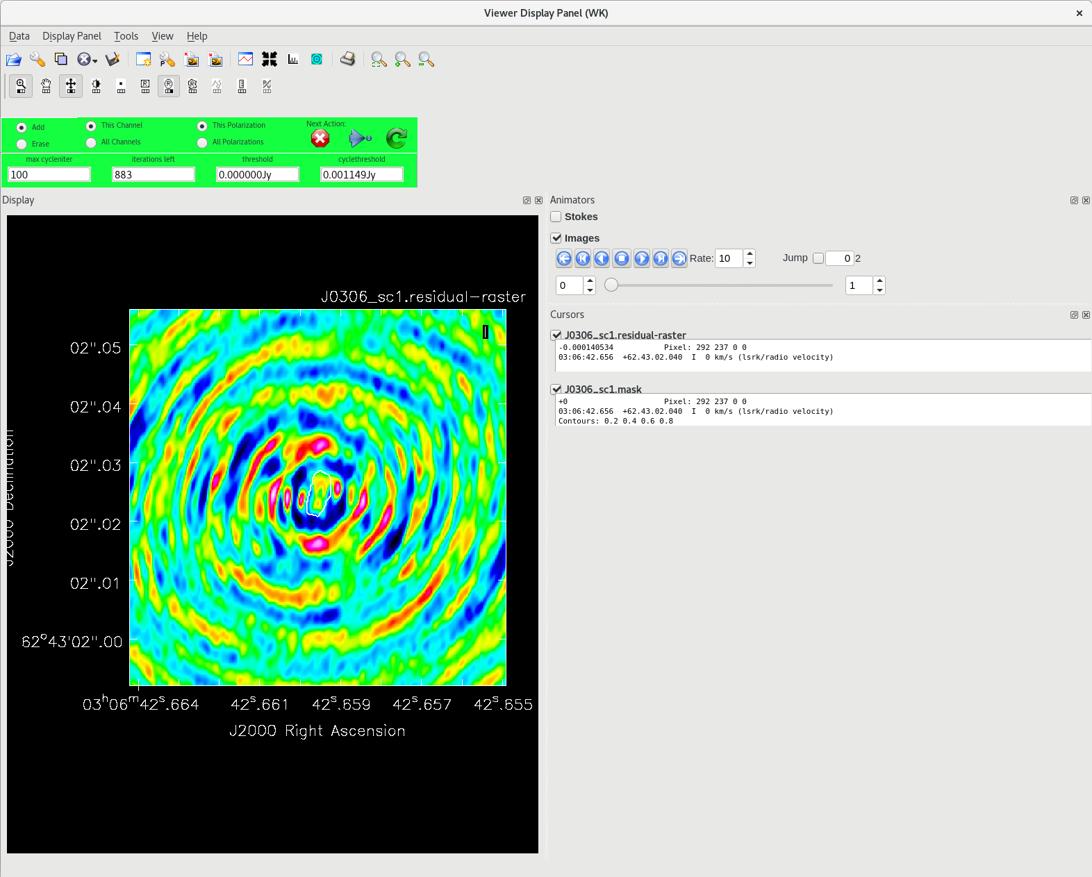
Running [https://casadocs.readthedocs.io/en/v6. | Running [https://casadocs.readthedocs.io/en/v6.6.5/api/tt/casatasks.imaging.tclean.html tclean] with ''interactive=True'' will open a new Viewer Display Panel where you can control the cleaning of the image. You should see that J0306+6243 is fairly point-like. Use the zoom tool to select the region around the source. Use the "polygon drawing" tool to draw a clean window around the source, excluding the stuff to the left and right of the bright source. Click on the "Continue deconvolution" button (the green circular arrow on the right). Check the residuals when the display updates. Stop cleaning when the area around the source looks noise-like. For example, if you notice positive and negative regions with similar magnitudes (e.g., +0.003 and -0.003) inside your clean window, that is probably a good time to stop cleaning. To stop the cleaning process, click the "stop deconvolving now" button (the red circle with the white "X"). It may take [https://casadocs.readthedocs.io/en/v6.6.5/api/tt/casatasks.imaging.tclean.html tclean] a while to finish and close. | ||
| Line 893: | Line 892: | ||
=== Tracking Improvement === | === Tracking Improvement === | ||
To ensure that self-calibration is actually helping to improve the quality of the images, you should track some image statistics. The most reliable way to do this is to define 2 boxes in the image; one box that contains the source ("on-source"), and one box that does not contain any part of the source ("off-source"). You can use [https://casadocs.readthedocs.io/en/v6. | To ensure that self-calibration is actually helping to improve the quality of the images, you should track some image statistics. The most reliable way to do this is to define 2 boxes in the image; one box that contains the source ("on-source"), and one box that does not contain any part of the source ("off-source"). You can use [https://casadocs.readthedocs.io/en/v6.6.5/api/tt/casaviewer.imview.html#casaviewer.imview imview] to inspect the image and determine where to place the on-source and off-source boxes. | ||
<source lang="python"> | <source lang="python"> | ||
| Line 907: | Line 906: | ||
</source> | </source> | ||
Once you have your on- and off-source boxes defined, use the task [https://casadocs.readthedocs.io/en/v6. | Once you have your on- and off-source boxes defined, use the task [https://casadocs.readthedocs.io/en/v6.6.5/api/tt/casatasks.information.imstat.html imstat] to gather some statistics about those regions. | ||
<source lang="python"> | <source lang="python"> | ||
#In CASA | #In CASA | ||
| Line 914: | Line 913: | ||
</source> | </source> | ||
Running [https://casadocs.readthedocs.io/en/v6. | Running [https://casadocs.readthedocs.io/en/v6.6.5/api/tt/casatasks.information.imstat.html imstat] will return several values in both the logger and the CASA terminal. The values of interest for the self-calibration process are the on-source peak value ("max"), the on-source total flux density ("flux"), and the off-source RMS value ("rms"). It is a <b>very</b> good idea to record each of these values for each image (including the first image without any self-calibration applied) as you proceed with self-calibration. Ideally, the on-source peak and total flux values will increase slightly and the off-source RMS will decrease significantly as you improve the calibration. However, be very suspicious of large increases (>10%) in flux density values, especially when the off-source RMS does not improve dramatically. | ||
For the first image of | For the first image of J0306+6243, the values should be fairly close to: | ||
<pre style="background-color: #E0FFFF;"> | <pre style="background-color: #E0FFFF;"> | ||
On-source: | On-source: | ||
| Line 928: | Line 927: | ||
=== Phase Self-Calibration === | === Phase Self-Calibration === | ||
Now that we have an initial model of the phase reference calibrator (from the image), we can begin the self-calibration process. In CASA, this is done with the [https://casadocs.readthedocs.io/en/v6. | Now that we have an initial model of the phase reference calibrator (from the image), we can begin the self-calibration process. In CASA, this is done with the [https://casadocs.readthedocs.io/en/v6.6.5/api/tt/casatasks.calibration.gaincal.html gaincal] task. | ||
<b>NOTE: </b>In the Basic Phase-referencing tutorial, we performed the self-calibration steps on the split dataset. In this tutorial, we are using the initial dataset (for reasons that will become obvious later). Therefore, we must remember to pre-apply all of the calibration tables during our self-calibration steps. | <b>NOTE: </b>In the Basic Phase-referencing tutorial, we performed the self-calibration steps on the split dataset. In this tutorial, we are using the initial dataset (for reasons that will become obvious later). Therefore, we must remember to pre-apply all of the calibration tables during our self-calibration steps. | ||
| Line 940: | Line 939: | ||
[[File:vlba_SpectralLine_selfcal_delays.png|300px|right|thumb|Figure 47: Plot of the delay self-calibration solutions vs time. Note that the vlaues are all small (the y-axis scale is in ns) and centered around zero.]] | [[File:vlba_SpectralLine_selfcal_delays.png|300px|right|thumb|Figure 47: Plot of the delay self-calibration solutions vs time. Note that the vlaues are all small (the y-axis scale is in ns) and centered around zero.]] | ||
When [https://casadocs.readthedocs.io/en/v6. | When [https://casadocs.readthedocs.io/en/v6.6.5/api/tt/casatasks.calibration.gaincal.html gaincal] finishes, check the logger window. You should see: | ||
<pre style="background-color: #fffacd;"> | <pre style="background-color: #fffacd;"> | ||
Finished solving. | Finished solving. | ||
| Line 972: | Line 971: | ||
Again, all the of the numbers match, which is what we want to see. | Again, all the of the numbers match, which is what we want to see. | ||
Inspect the phase solution table with [https://casadocs.readthedocs.io/en/v6. | Inspect the phase solution table with [https://casadocs.readthedocs.io/en/v6.6.5/api/tt/casaplotms.plotms.html plotms]. | ||
<source lang="python"> | <source lang="python"> | ||
#In CASA | #In CASA | ||
| Line 987: | Line 986: | ||
</source> | </source> | ||
Make a new image after the improved phase calibration using [https://casadocs.readthedocs.io/en/v6. | Make a new image after the improved phase calibration using [https://casadocs.readthedocs.io/en/v6.6.5/api/tt/casatasks.imaging.tclean.html tclean] just as we did previously. Remember to use a new ''imagename'' for this new image of the phase self-calibrated data. | ||
<source lang="python"> | <source lang="python"> | ||
#In CASA | #In CASA | ||
| Line 993: | Line 992: | ||
</source> | </source> | ||
Once you have created the new image, check for improvement with [https://casadocs.readthedocs.io/en/v6. | Once you have created the new image, check for improvement with [https://casadocs.readthedocs.io/en/v6.6.5/api/tt/casatasks.information.imstat.html imstat]. As long as you did not change the ''imsize'' or ''cell'' parameters, you can use the same on- and off-source boxes that we defined earlier. | ||
<source lang="python"> | <source lang="python"> | ||
#In CASA | #In CASA | ||
| Line 1,000: | Line 999: | ||
</source> | </source> | ||
For the second image of | For the second image of J0306+6243, the values should be fairly close to: | ||
<pre style="background-color: #E0FFFF;"> | <pre style="background-color: #E0FFFF;"> | ||
On-source: | On-source: | ||
'flux': 0. | 'flux': 0.167 | ||
'max': 0. | 'max': 0.172 | ||
Off-source: | Off-source: | ||
'rms': 0.00057 | 'rms': 0.00057 | ||
| Line 1,028: | Line 1,027: | ||
[[File:vlba_SpectralLine_ampselfcal_AmpvTime.png|300px|right|thumb|Figure 49: Plot of the amplitude and phase self-calibration solutions vs time. Note that the values are generally near 1.0, although some telescopes have larger corrections.]] | [[File:vlba_SpectralLine_ampselfcal_AmpvTime.png|300px|right|thumb|Figure 49: Plot of the amplitude and phase self-calibration solutions vs time. Note that the values are generally near 1.0, although some telescopes have larger corrections.]] | ||
We should take a look at the solutions on each telescope using [https://casadocs.readthedocs.io/en/v6. | We should take a look at the solutions on each telescope using [https://casadocs.readthedocs.io/en/v6.6.5/api/tt/casaplotms.plotms.html plotms]. | ||
<source lang="python"> | <source lang="python"> | ||
#In CASA | #In CASA | ||
| Line 1,055: | Line 1,054: | ||
</source> | </source> | ||
For the final image of | For the final image of J0306+6243, the values should be fairly close to: | ||
<pre style="background-color: #E0FFFF;"> | <pre style="background-color: #E0FFFF;"> | ||
On-source: | On-source: | ||
'flux': 0. | 'flux': 0.189 | ||
'max': 0. | 'max': 0.177 | ||
Off-source: | Off-source: | ||
'rms': 0.00023 | 'rms': 0.00023 | ||
| Line 1,095: | Line 1,094: | ||
<source lang="python"> | <source lang="python"> | ||
#In CASA | #In CASA | ||
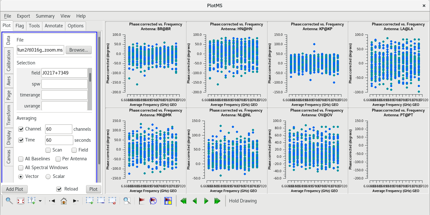
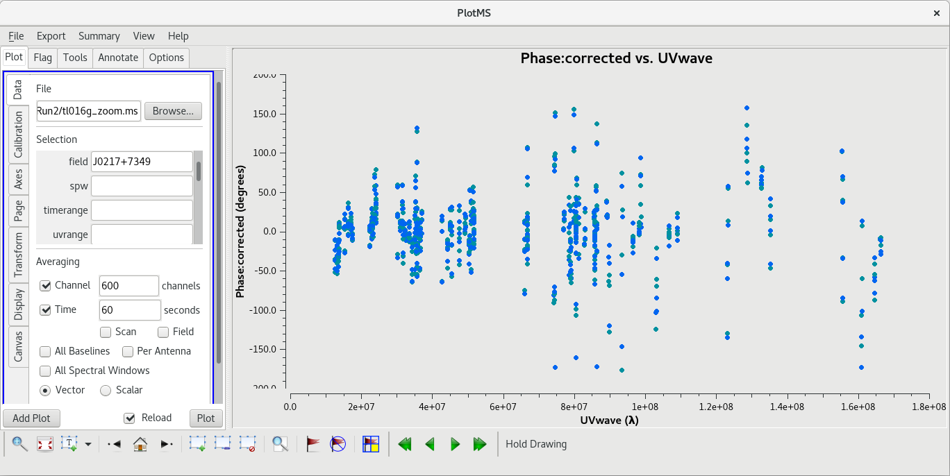
plotms(vis='tl016g_zoom.ms', xaxis='frequency', yaxis='phase', ydatacolumn=' | plotms(vis='tl016g_zoom.ms', xaxis='frequency', yaxis='phase', ydatacolumn='corrected', field='J0217+7349', antenna='*&*', scan='92', correlation='rr,ll', gridrows=2, gridcols=4, iteraxis='antenna', coloraxis='corr', avgchannel='60', avgtime='60') | ||
</source> | </source> | ||
| Line 1,117: | Line 1,116: | ||
<source lang="python"> | <source lang="python"> | ||
#In CASA | #In CASA | ||
split(vis='tl016g_zoom.ms', outputvis=' | split(vis='tl016g_zoom.ms', outputvis='w3oh_zoom.ms', field='W3OH', antenna='*&*', datacolumn='corrected') | ||
</source> | </source> | ||
| Line 1,125: | Line 1,124: | ||
<source lang="python"> | <source lang="python"> | ||
#In CASA | #In CASA | ||
plotms(vis='tl016g_zoom.ms', | plotms(vis='tl016g_zoom.ms', field='W3OH', scan='87', xaxis='frequency', yaxis='amp', coloraxis='corr', iteraxis='antenna') | ||
</source> | </source> | ||
[[File:vlba_SpectralLine_W3OH_ampvfreq.png|300px|right|thumb|Figure 52: Amplitude vs frequency for the calbrated zoom band data on W3OH, scan 87.]] | [[File:vlba_SpectralLine_W3OH_ampvfreq.png|300px|right|thumb|Figure 52: Amplitude vs frequency for the calbrated zoom band data on W3OH, scan 87.]] | ||
You should see a large spread in the frequencies of the maser line. This is due to different regions of W3OH having different velocities, and therefore different Doppler shifts. To properly image the | You should see a large spread in the frequencies of the maser line. This is due to different regions of W3OH having different velocities, and therefore different Doppler shifts. To properly image the maser lines, we will need to know both the location in the field and the frequency of the lines at that location. | ||
Now, we will finally make images of the masers. There are a few differences between making these images and when we made continuum images of the phase reference calibrator. Namely, we will use ''specmode='cube'''. | Now, we will finally make images of the masers. There are a few differences between making these images and when we made continuum images of the phase reference calibrator. Namely, we will use ''specmode='cube'''. | ||
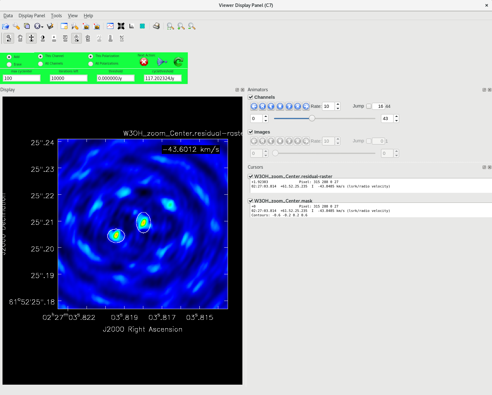
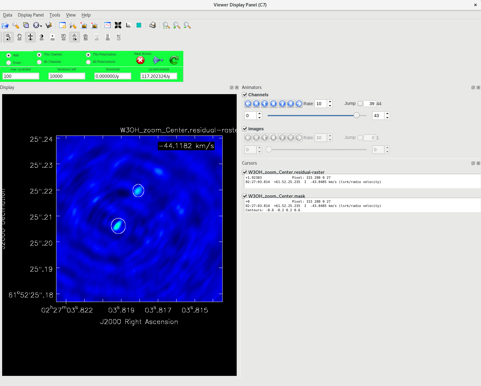
There are actually many masers in our field of view. To make one image with all of them, you will need a large amount of memory (RAM). This should only be attempted on an NRAO cluster node, or a computer with at least 32 GB of RAM (preferably 64 GB). | There are actually many masers in our field of view. To make one image with all of them, you will need a large amount of memory (RAM). This should only be attempted on an NRAO cluster node, or a computer with at least 32 GB of RAM (preferably 64 GB). Also, be warned that it may take you all day to make one image. For those who are interested in trying to make this large image cube, here are the reocmmended [https://casadocs.readthedocs.io/en/v6.6.5/api/tt/casatasks.imaging.tclean.html tclean] inputs: ''vis='w3oh_zoom.ms', field='W3OH', spw='0:240~440', imsize=[1620], cell=['0.2mas'], stokes='I', specmode='cube', restfreq='6668.5192MHz', deconvolver='hogbom', weighting='natural', niter=100000, interactive=True, savemodel='none'.'' Good luck. | ||
For this tutorial, we will cheat a little and make two small image cubes of select maser regions rather than one huge image cube. | |||
<b>A NOTE ON BEST PRACTICES: </b>When making VLBA image cubes of targets like masers, it is best to create separate clean masks for each spectral channel (this is part of the reason that making the big image of the entire field might take all day; you need to create several unique masks for each spectral channel). Because the maser line has a Doppler shift, it will not be equally bright in each spectral channel and its position is different in each spectral channel. If you define a single clean mask for all specrtral channels, you could clean noise and/or artifacts in the channels without maser emission. However, if the area of interest is small enough that the restoring beam sidelobes are not going to contaminate other parts of the image, you can get away with only defining one clean mask for all spectral channels. | |||
We will start with something relatively easy. There is a region in the southern part of our target region with a single bright maser confined to a relatively small number of spectral channels. The region is also small enough that we should be able to avoid problems with the sidelobes, so we can define a single clean mask for all of the spectral channels. We will use [https://casadocs.readthedocs.io/en/v6.6.5/api/tt/casatasks.imaging.tclean.html tclean] in the interactive mode and set ''specmode='cube'''. We will also need to shift the center of the image to the location of the maser using the ''phasecenter'' parameter. Finally, we need to provide the rest frequency of the maser line, which is 6668.5192MHz. | |||
<source lang="python"> | |||
#In CASA | |||
tclean(vis='w3oh_zoom.ms', field='W3OH', spw='0:276~304', imagename='W3OH_zoom_South', imsize=[200], cell=['0.2mas'], phasecenter='J2000 02:27:03.823 +61.52.25.084', stokes='I', specmode='cube', restfreq='6668.5192MHz', deconvolver='hogbom', weighting='natural', niter=10000, interactive=True, savemodel='none') | |||
</source> | |||
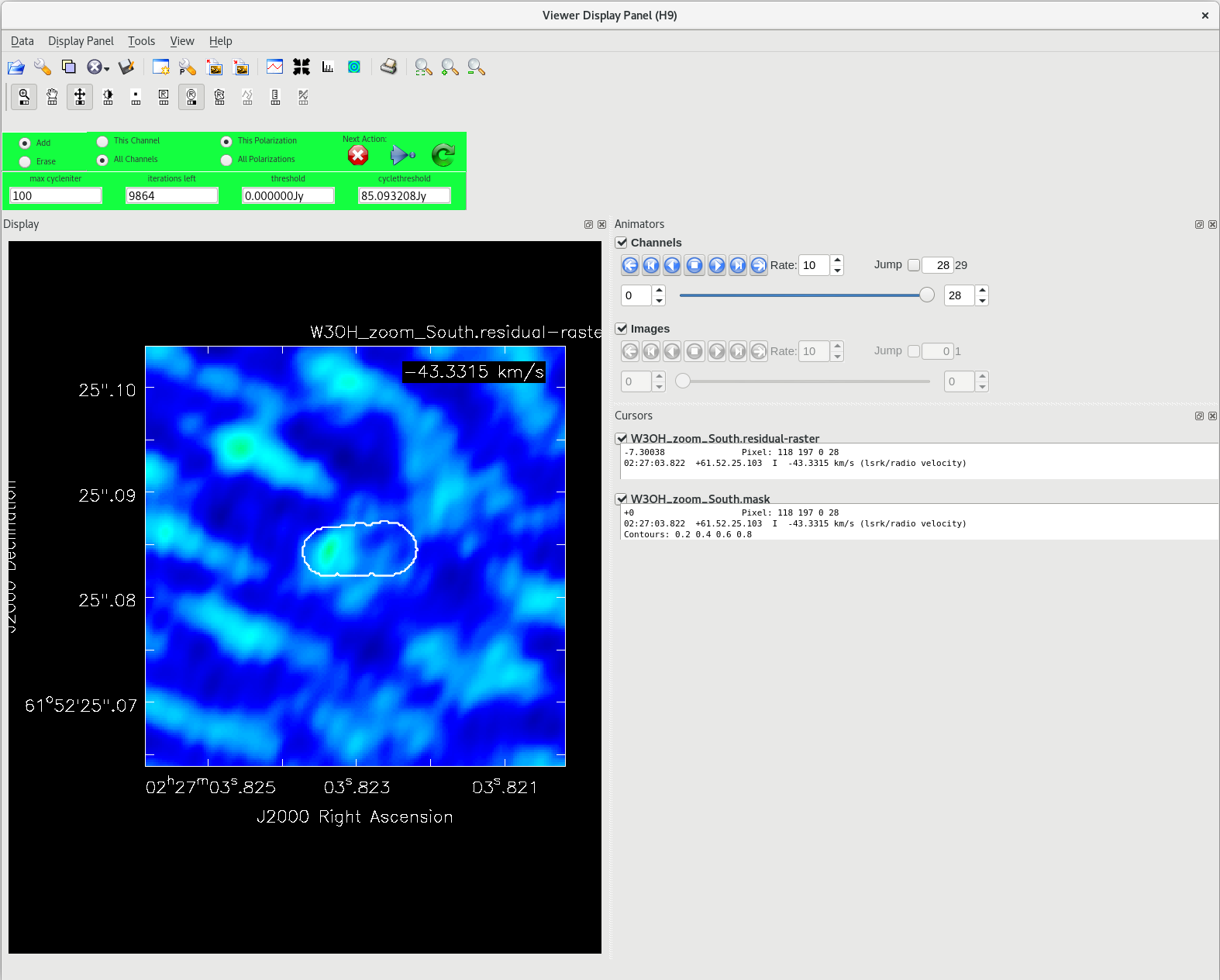
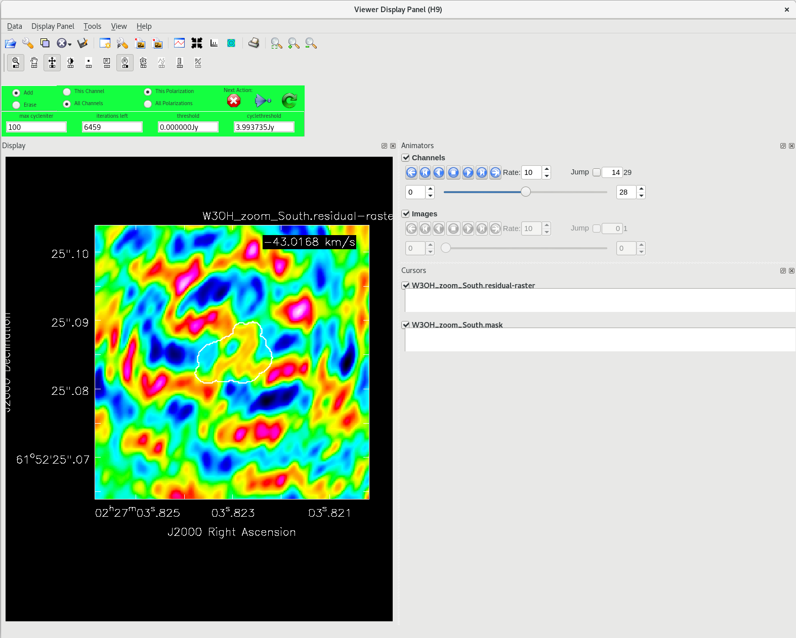
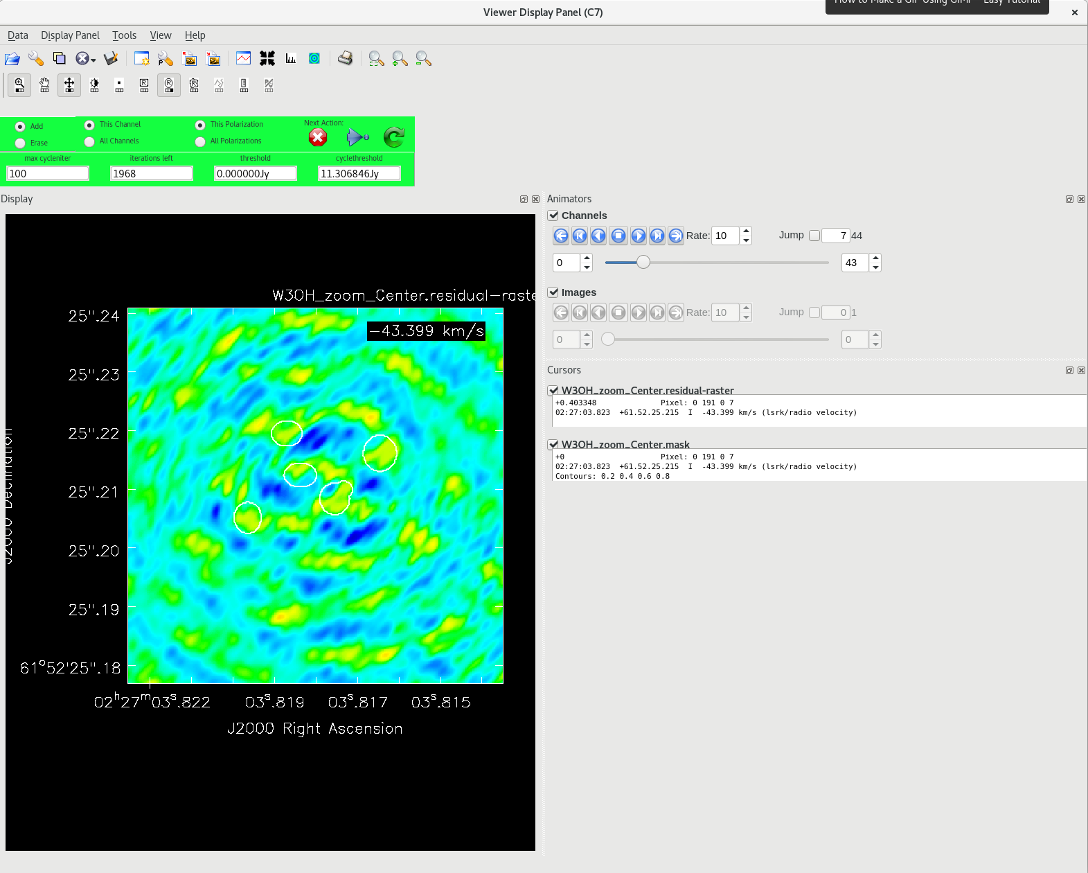
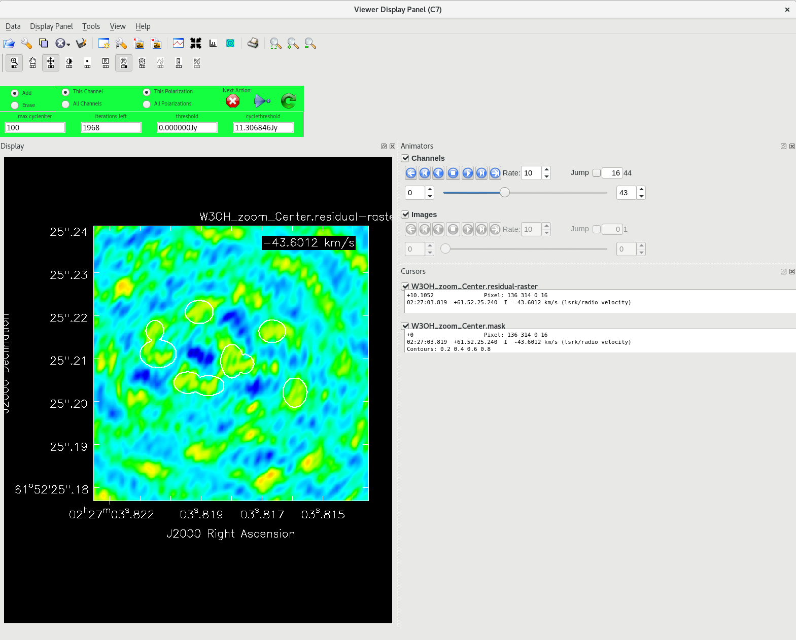
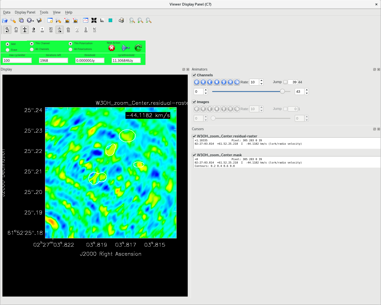
The interactive clean GUI will open showing the first spectral channel in our selected range. You should not see anything in there, yet. In the right-hand panel under "Channels", click on the Play button to step through all of the channels we have selected for this cube. You should see the maser line become very obvious in fourth or fifth spectral channel. It will appear to move from right to left as the display steps through the spectral channels. Notice that some artifacts start to become obvious in the tenth or eleventh spectral channel. These are the sidelobes in our beam. Fortunately, the maser in this region is confined to a region small enough that the sidelobes will not overlap any of the maser emission. So, we can be lazy and just define a single clean mask for all of the spectral channels. Click the Stop button once you have watched the display step through all of the channels a few times. | |||
In the green region in the upper left, select "All Channels". Any time we add a clean mask in one spectral channel, it will apply to all spetral channels. Use the Forward Step button (right-pointing triangle with vertical line on right-hand side) to step through the spectral channels until you get to one where the maser emission is obvious. Use you favorite mask drawing tool (I tend to use the Ellipse tool for this one) to draw the first clean mask. Step through more channels and add mask components that cover all of the maser emission in every spectral channel. Once you have a mask defined and you are confident it covers all of the obvious maser emission, click the "Continue deconvolution" button (circular green arrow in upper right of the green region) to start the clean process. | |||
{| | |||
| [[File: vlba_SpectralLine_W3OHsouth_firstmask.png|300px|left|thumb|Figure 53: Dirty image of W3OH southern region with first clean mask defined.]] | |||
| [[File: vlba_SpectralLine_W3OHsouth_mask.png|300px|right|thumb|Figure 54: Dirty image of W3OH southern region with clean mask defined, ready to start cleaning.]] | |||
|} | |||
When the first round of cleaning finishes, you will get a new set of residual images. Step through them and enlarge your clean mask to get all of the maser emission you can see now that the noise is reduced. Once your larger clean mask is set, click the "Continue deconvolution" button again to continue cleaning. Go through this process until the maser region is noise-like in all spectral channels. When you are done cleaning, click the "Stop deconvolving now" button (red cirlce with the white 'X' in the middle). Several new files will be created in you directory, including the image file "W3OH_zoom_South.image". | |||
{| | |||
| [[File: vlba_SpectralLine_W3OHsouth_secondmask.png|300px|left|thumb|Figure 55: Residual image of W3OH southern region after first round of cleaning. The clean mask has been updated based on the additional flux now evident.]] | |||
| [[File: vlba_SpectralLine_W3OHsouth_stopclean.png|300px|right|thumb|Figure 56: Residual image of W3OH southern region after several iterations of cleaning. The maser region looks noise-like in all spectral channels, so it is time to stop cleaning.]] | |||
|} | |||
You can inspect the image cube with the CASA viewer or with CARTA. For this tutorial, we will use the viewer | |||
<source lang="python"> | |||
#In CASA | |||
imview | |||
</source> | |||
This will open a new window. Click on the File icon (just below "Data" in the top row) and look for your image cube file. Select the image cube file and click "raster image". This will display a colorscale version of the image cube. Click the Play button to step through all of the spectral windows. You should see the maser get brighter and move from right to left in the display. | |||
Now that we have an image cube, let's do a little spectral analysis. We'll make a position-velocity diagram. In order to do this, we will need to describe a "slit" (a straight line in pixel space) along the maser's path as we step through the spectral channels. Our maser appears to move almost perfectly horizontally, so the y pixel position should not change much. Looking at the lower spectral channels, we will start our "slit" at x=126, y=102 (just to the west/right of the maser in the lower spectral channels). Stepping through the spectral channels, we will end our slit at x=79, y=102. Use the CASA task [https://casadocs.readthedocs.io/en/v6.6.5/api/tt/casatasks.analysis.impv.html impv] to create the position-velocity diagram. | |||
<source lang="python"> | |||
#In CASA | |||
impv(imagename='W3OH_zoom_South.image', outfile='W3OH_zoom_South_PV1.image', mode='coords', start=[126,102], end=[79,102]) | |||
</source> | |||
This will make a new file called "W3OH_zoom_South_PV1.image", which you can open with the CASA viewer. | |||
{| | |||
| [[File: vlba_SpectralLine_W3OHsouth_PV1.png|300px|left|thumb|Figure 57: Position-velocity diagram for the W3OH southern region maser.]] | |||
|} | |||
Now that we have done an easy example of imaging a maser region, let's try something more challenging. We will make an image cube of a region near the center of our pointing. This region has several masers, and they are separated in both space and frequency. Because there are multiple masers in the area and the region is larger than for our first image, we will need to make separate clean masks for each spectral channel. | |||
<source lang="python"> | |||
#In CASA | |||
tclean(vis='w3oh_zoom.ms', field='W3OH', spw='0:300~342', imagename='W3OH_zoom_Center', imsize=[320], cell=['0.2mas'], phasecenter='J2000 02:27:03.818 +61.52.25.209', stokes='I', specmode='cube', restfreq='6668.5192MHz', deconvolver='hogbom', weighting='natural', niter=10000, interactive=True, savemodel='none') | |||
</source> | |||
{| | |||
| [[File: vlba_SpectralLine_W3OHcenter_initialmaskch7.png|300px|left|thumb|Figure 58: Dirty image of W3OH central region lower spectral channel with initial clean mask defined.]] | |||
| [[File: vlba_SpectralLine_W3OHcenter_initialmaskch16.png|300px|right|thumb|Figure 59: Dirty image of W3OH central region mid spectral channel with initial clean mask defined.]] | |||
| [[File: vlba_SpectralLine_W3OHcenter_initialmaskch39.png|300px|right|thumb|Figure 60: Dirty image of W3OH central region upper spectral channel with initial clean mask defined.]] | |||
|} | |||
Make sure that you have "This Channel" selected (in the green region) so that you create clean masks for each spectral channel separately. When stepping through the spectral channels for the dirty image, it may not be obvious what is a maser and what is an sidelobe artifact. To start with, only mask the brightest objects in a spectral channel. After cleaning a little, it will become more obvious what is a real maser. You will need to update the clean masks each time you get a new residual image. Keep an eye on the Remaining Iterations box in the interactive clean window. You will likely see the number get pretty low before you decide to stop cleaning. If you run out of iterations, you can start [https://casadocs.readthedocs.io/en/v6.6.5/api/tt/casatasks.imaging.tclean.html tclean] again and pick up where you left off as long as ''restart=True'' (which is the default) and all of the image parameters (''imagename'', ''imsize'', ''cell'', etc.) are the same as the previous execution. | |||
{| | |||
| [[File: vlba_SpectralLine_W3OHcenter_finalmaskch7.png|300px|left|thumb|Figure 61: Residual image of W3OH central region lower spectral channel after multiple iterations of cleaning, with final clean mask defined.]] | |||
| [[File: vlba_SpectralLine_W3OHcenter_finalmaskch16.png|300px|right|thumb|Figure 62: Residual image of W3OH central region mid spectral channel after multiple iterations of cleaning, with final clean mask defined.]] | |||
| [[File: vlba_SpectralLine_W3OHcenter_finalmaskch39.png|300px|right|thumb|Figure 63: Residual image of W3OH central region upper spectral channel after multiple iterations of cleaning, with final clean mask defined.]] | |||
|} | |||
Once you are done cleaning and have created your image cube of the central region, take a look at it with the CASA viewer. | |||
<source lang="python"> | |||
#In CASA | |||
imview | |||
</source> | |||
Open the file "W3OH_zoom_Center.image" as a raster image. Click the Play button to step through the spectral channels. You should see a complicated region with several masers appearing, moving, and disappearing. | |||
Congratulations! You have calibrated and imaged a VLBA spectral line observation in CASA! | |||
Latest revision as of 16:41, 5 November 2024
This CASA Guide is for Version 6.6.5 of CASA. If you are using a later version of CASA and this is the most recent available guide, then you should be able to use most, if not all, of this tutorial.
SPECIAL NOTE FOR DRAFT VERSION: To follow the tutorial, you will need to use CASA 6.6.5 in order to perform the EOP correction.
Overview
This CASA Guide describes the procedure for calibrating a phase-referenced VLBA observation of methanol masers in W3OH. The data were taken specifically for this tutorial. The observation made use of the DDC observing personality, using dual polarization with one spectral window in each polarization. The spectral window has a bandwidth of 32 MHz divided into 640 spectral channels centered at 6668 MHz for the methanol maser line. In addition, there is a "zoom" band file with very high spectral resolution centered on the maser line. The methanol maser line itself has a rest frequency of 6668.5192 MHz (e.g., Muller, Menten & Mader 2004).
This tutorial will focus on calibrating the data and creating a continuum (Stokes I) image of the phase reference calibrator and image cubes of some of the stronger the masers in W3OH.
Those who have already worked through the VLBA Basic Phase-referencing tutorial will recognize that many of the calibration steps in this tutorial are very similar (sometimes identical). In general, the initial calibration (data ingestion through amplitude calibration) of spectral line data are the same. The major differences between continuum and spectral line projects are in the self-calibration steps, applying calibration from the primary file to the zoom file, target imaging, and specific spectral line analysis steps.
Please note that CASA should be used with caution when calibrating VLBA data. At the current time, CASA should only be used to calibrate relatively simple VLBA observations (basic continuum, simple phase-referenced, etc.). In particular, CASA is currently not recommended for calibrating the following types of VLBA observations:
- Polarimetric — Calibration of resolved polarized sources is not yet available in CASA.
- Astrometric — Pulse-cal tone corrections are not yet available in CASA.
- Spectral line projects requiring fringe-rate mapping — Fringe-rate mapping is not yet available in CASA.
- Low Frequency (<4 GHz) — Total electron content (TEC) corrections have not yet been verified to work correctly for VLBI observations in CASA. Also, note that many C-band (4 to 8 GHz) VLBA observations will benefit from TEC corrections.
- VLBA+Y27 or other VLBA+ arrays that require the use of antab files — CASA does not currently support the use of antab files for ingesting calibration data (system temperatures, gain curves, etc.)
If your observation involves any of the above, you should use AIPS to calibrate your data.
A note on pre-DiFX data: Starting with CASA 6.6.4, VLBA data correlated with the hardware correlator (prior to December 2009) can be imported into CASA Measurement Sets with importfitsidi. However, users should take great care in using CASA to calibrate these data because the data weights may not be correct, especially for the oldest data and data with the Hanning taper applied. Warning messages will appear for data with the Hanning taper applied and some other known problems, but not every case has been tested.
A note on Earth Orientation Parameter corrections: Starting with CASA 6.6.5 (Fall 2024), it is possible to correct the Earth Orientation Parameters (EOP) in a VLBA observation. Unlike with AIPS, CASA users will need to download the EOP file themselves. These files can be obtained from NASA using the following command: curl -u anonymous:<your-email-address> --ftp-ssl ftp://gdc.cddis.eosdis.nasa.gov/vlbi/gsfc/ancillary/solve_apriori/usno_finals.erp > /<path>/<to>/<file>/usno_finals.erp
A note on VLBA+Y1 observations: It is currently possible to calibrate VLBA+Y1 (VLBA and single VLA antenna) in CASA. Any data taken after 2022 July 06 should work with minimal extra steps (namely, checking that the Y1 antenna diameter is correct). VLBA+Y1 data observed prior to 2022 July 06 may not include the system temperature and/or gain curve values need for calibration. For these data sets, refer to VLBA Scientific Memo 39 for details on how to prepare the data for calibration in either CASA or AIPS.
Mac OS 13 and OS 14 WARNING: The CASA Viewer will not work on Mac OS 13, OS 14, or later. The tclean task relies on the CASA Viewer for interactive cleaning. So, users with Mac OS 13, OS 14, or newer will not be able to make their images interactively in CASA. Because interactive cleaning is extremely important for creating image cubes from VLBA spectral line observations, users running Mac OS 13, OS 14, or later are strongly encouraged to use an alternate software package to create their images (AIPS). Alternatively, Mac users can request access to Linux-based NRAO computing resources by submitting a helpdesk ticket (in the Department field, select "VLA/GBT/VLBA Archive and Data Retrieval" and request a guest account to calibrate and image VLBA data).
How to Use This CASA Guide
There are a number of possible ways to run CASA, described in more detail in Getting Started in CASA. In brief, there are at least three different ways to use CASA:
- Interactively examining task inputs. In this mode, one types taskname to load the task, inp to examine the inputs, and go once those inputs have been set to your satisfaction. Allowed inputs are shown in blue and bad inputs are colored red. The input parameters themselves are changed one by one, e.g., selectdata=True. Screenshots of the inputs to various tasks used in the data reduction below are provided, to illustrate which parameters need to be set. More detailed help can be obtained on any task by typing help taskname. Once a task is run, the set of inputs are stored and can be retrieved via tget taskname; subsequent runs will overwrite the previous tget file.
- Pseudo-interactively via task function calls. In this case, all of the desired inputs to a task are provided at once on the CASA command line. This tutorial is made up of such calls, which were developed by looking at the inputs for each task and deciding what needed to be changed from default values. For task function calls, only parameters that you want to be different from their defaults need to be set.
- Non-interactively via a script. A series of task function calls can be combined together into a script, and run from within CASA via execfile('scriptname.py'). This and other CASA Tutorial Guides have been designed to be extracted into a script via the script extractor by using the method described at the Extracting_scripts_from_these_tutorials page. Should you use the script generated by the script extractor for this CASA Guide, be aware that it will require some small amount of interaction related to the plotting, occasionally suggesting that you close the graphics window and hitting return in the terminal to proceed. It is in fact unnecessary to close the graphics windows (it is suggested that you do so purely to keep your desktop uncluttered).
If you are a relative novice or just new to CASA, it is strongly recommended to work through this tutorial by cutting and pasting the task function calls provided below after you have read all the associated explanations. Work at your own pace, look at the inputs to the tasks to see what other options exist, and read the help files. Later, when you are more comfortable, you might try to extract the script, modify it for your purposes, and begin to reduce other data.
NOTE: It is not recommended to use scripts to generate "science-ready" VLBA data products. Nearly all VLBA observations will require some amount of hands-on calibration. Calibration and imaging scripts should only be used as "first pass" attempts at calibration, which can be useful to determine if the observation resulted in a detection and to identify problems in the data.
Obtaining the Data
This Guide is intended to cover the entire process one would follow for calibrating their own VLBA observation. Therefore, we will start with a FITS-IDI file rather than a Measurement Set. The primary FITS-IDI files for this Guide is: TL016G.IDIFITS (right-click and select "Save Link As..."; file size: 2.5 GB). Additionally, you will need to download the zoom band file containing the very high spectral resolution data: TL016GZOOM.IDIFITS (files size: 6.3 GB)
Alternatively, you may download the data from the NRAO Archive. In the archive search inputs, enter "TL016" in the Project Code field. Expand the results for TL016G and look for the files VLBA_TL016G_tl016g_BIN0_SRC0_0_240725T190341.idifits (the primary data file) and VLBA_TL016G_tl016gzoomrecor3_BIN0_SRC0_0_240805T135429.idifits (the "zoom" band file). Select the file, click "Download", and follow the instructions. Once you have downloaded the FITS-IDI file from the archive, it will be helpful to change the filenames to "TL016G.IDIFITS" and "TL016GZOOM.IDIFITS".
The Observing Log
Before diving into the calibration, it is always a good idea to look over the observing log to check for notes from the operators that can inform us about potential issues with the data (missing stations, bad weather, etc.). These logs are always emailed to the PI's of an observation, but you can also access them later from the NRAO's vlbiobs fileserver. To locate an observing log, first find the directory for observing month and the last two digits of the year (for the observation used in this Guide, that directory is jul24 for July 2024). Once inside the proper month+year directory, look for the project code (in this case, tl016g). Look for a file named <project code>log.vbla (tl016glog.vlba).
The observing log for this particular observation looked like this:
VERY LONG BASELINE ARRAY OBSERVING LOG
--------------------------------------
Project:        TL016G
Observer:       Linford, Justin
Project type:   TEST
Obs filename:   tl016g.vex
Date/Day:       2024JUL14/196
Ants Scheduled: SC HN NL FD LA PT KP OV BR MK

=UT-Time===Comment===============================================MF#===%AD==AMD=
           Operator: Alan Kerr
     1230  Begin
1230-1700 *SC out, rail work. WO-19635                           AMECH  100  270
1230-1700 *FD out, bad ACU power supply. WO-21598                PS     100  270
     1333  New Operator: Paul Padilla
     1700  End.


Downtime Summary:
	Total downtime : 540 min
	Percentage downtime of observing: 20.0%
	Average downtime per hour : 12.0 min

    Total scheduled observing time (# Antennas): 2700 min (10)

Notes:
    * = Entries where data was affected.
    % = Entries where data may have been affected.
    & = Entries where the site tech was called out.
  WEA = Weather entries.
  MF# = Maintenance form or major downtime category associated with a problem.
  %AD = The percentage of an antenna affected by a problem.
  AMD = Total antenna-minutes downtime for a problem.
 Tsys = System Temperature (TP/SP x Tcal/2)
  ACU = Antenna Control Unit
  FRM = Focus/Rotation Mount
  RFI = Radio Frequency Interference
   CB = Circuit Breaker
From the log, we can see that two stations, FD and SC, did not participate. No other issues were reported by the operators.
Creating the Measurement Set
Before beginning our data reduction, we must start CASA. If you have not used CASA before, some helpful tips are available on the Getting Started in CASA page. Remember to start CASA in the directory containing the observation data.
Once you have CASA up and running, it is time to get the data into a format that CASA can use. Unlike VLA data, a VLBA observation is only available as a FITS-IDI file and cannot be downloaded as a CASA Measurement Set. So, the first step in calibrating a VLBA observation with CASA is to create a Measurement Set from the FITS-IDI file. To do this, we will use the task importfitsidi:
# In CASA
importfitsidi(fitsidifile='TL016G.IDIFITS', vis='tl016g.ms', constobsid=True, scanreindexgap_s=15)
The scanreindexgap_s parameter is used to reconstruct scan boundaries in those cases where sources do not change between scans. In general, it is good to set scanreindexgap_s to some non-zero number to help CASA properly organize the scan list. The recommended value is 15 seconds, but smaller values may work as well (although you probably don't want to go much shorter than about 5 seconds). If you find that the resulting MS contains too few scans, run importfitsidi again with scanreindexgap_s set to a smaller number. If your MS has too many scans, especially multiple scans on the same source when you think it should just be one scan, run importfitsidi again with scanreindexgap_s set to a larger number.
NOTE: You may see warnings in the CASA window like "Table not yet implemented" and "Keyword has wrong data type". This is normal behavior for VLBA data and due to the fact that CASA does not yet handle the pulse-cal tone data in the FTIS-IDI file. Just ignore them. However, do not ignore any SEVERE warnings, as these can indicate there are serious problems with the data.
Inspecting the Data
Now that we have a Measurement Set, we need to look things over. This is where we will start to identify possible problems, but also find reliable antennas to use as the reference antenna.
The Observation Summary
It will be useful later to have the basic information about the observation. The task listobs will return a list of all the scans, the sources observed, which stations were used, and the frequency setup. It is possible to run listobs in two ways: printing information in the CASA logger, or saving the information to a file.
To simply display the information in the CASA logger:
#In CASA
listobs(vis='tl016g.ms')
You should see the listobs output in the CASA logger window:
================================================================================
MeasurementSet Name: /export/home/stibbons/CASA_VLBI/Tutorial/SpectralLine/Run1/tl016g.ms MS Version 2
================================================================================
Observer: PLUTO Project: TL016G
Observation: VLBA
Data records: 245996 Total elapsed time = 16154 seconds
Observed from 14-Jul-2024/12:31:00.0 to 14-Jul-2024/17:00:14.0 (UTC)
ObservationID = 0 ArrayID = 0
Date Timerange (UTC) Scan FldId FieldName nRows SpwIds Average Interval(s) ScanIntent
14-Jul-2024/12:31:00.0 - 12:35:00.0 1 0 J0102+5824 4320 [0] [2]
12:35:34.0 - 12:39:42.0 2 1 J0217+7349 4341 [0] [2]
12:40:02.0 - 12:41:16.0 3 2 J0306+6243 1228 [0] [2]
12:41:32.0 - 12:43:34.0 4 3 W3OH 2170 [0] [2]
12:43:50.0 - 12:44:50.0 5 2 J0306+6243 1054 [0] [2]
12:45:07.0 - 12:47:09.0 6 3 W3OH 2170 [0] [2]
12:47:24.0 - 12:48:26.0 7 2 J0306+6243 1082 [0] [2]
12:48:41.0 - 12:50:43.0 8 3 W3OH 2155 [0] [2]
12:50:59.0 - 12:52:01.0 9 2 J0306+6243 1083 [0] [2]
12:52:17.0 - 12:54:19.0 10 3 W3OH 2155 [0] [2]
12:54:34.0 - 12:55:36.0 11 2 J0306+6243 1083 [0] [2]
12:55:52.0 - 12:57:54.0 12 3 W3OH 2163 [0] [2]
12:58:09.0 - 12:59:11.0 13 2 J0306+6243 1082 [0] [2]
12:59:27.0 - 13:01:29.0 14 3 W3OH 2166 [0] [2]
13:01:44.0 - 13:02:46.0 15 2 J0306+6243 1078 [0] [2]
13:03:02.0 - 13:05:04.0 16 3 W3OH 2158 [0] [2]
13:05:19.0 - 13:06:21.0 17 2 J0306+6243 1086 [0] [2]
13:06:37.0 - 13:08:39.0 18 3 W3OH 2157 [0] [2]
13:08:55.0 - 13:09:57.0 19 2 J0306+6243 1086 [0] [2]
13:10:12.0 - 13:12:14.0 20 3 W3OH 2166 [0] [2]
13:12:29.0 - 13:13:31.0 21 2 J0306+6243 1065 [0] [2]
13:13:46.0 - 13:15:50.0 22 3 W3OH 2181 [0] [2]
13:16:04.0 - 13:17:06.0 23 2 J0306+6243 1065 [0] [2]
13:17:21.0 - 13:19:25.0 24 3 W3OH 2178 [0] [2]
13:19:39.0 - 13:20:41.0 25 2 J0306+6243 1075 [0] [2]
13:20:56.0 - 13:23:00.0 26 3 W3OH 2191 [0] [2]
13:23:14.0 - 13:24:18.0 27 2 J0306+6243 1114 [0] [2]
13:24:32.0 - 13:26:34.0 28 3 W3OH 2158 [0] [2]
13:26:49.0 - 13:27:53.0 29 2 J0306+6243 1105 [0] [2]
13:28:07.0 - 13:30:09.0 30 3 W3OH 2148 [0] [2]
13:30:24.0 - 13:31:28.0 31 2 J0306+6243 1101 [0] [2]
13:31:42.0 - 13:33:44.0 32 3 W3OH 2149 [0] [2]
13:33:59.0 - 13:35:03.0 33 2 J0306+6243 1114 [0] [2]
13:35:17.0 - 13:37:19.0 34 3 W3OH 2158 [0] [2]
13:37:34.0 - 13:38:38.0 35 2 J0306+6243 1110 [0] [2]
13:38:52.0 - 13:40:54.0 36 3 W3OH 2157 [0] [2]
13:41:09.0 - 13:42:13.0 37 2 J0306+6243 1110 [0] [2]
13:42:27.0 - 13:44:29.0 38 3 W3OH 2154 [0] [2]
13:44:44.0 - 13:45:46.0 39 2 J0306+6243 1082 [0] [2]
13:46:01.0 - 13:48:05.0 40 3 W3OH 2194 [0] [2]
13:48:19.0 - 13:49:21.0 41 2 J0306+6243 1078 [0] [2]
13:49:36.0 - 13:51:40.0 42 3 W3OH 2191 [0] [2]
13:51:54.0 - 13:52:56.0 43 2 J0306+6243 1080 [0] [2]
13:53:11.0 - 13:55:13.0 44 3 W3OH 2160 [0] [2]
13:55:28.0 - 13:56:32.0 45 2 J0306+6243 1111 [0] [2]
13:57:03.0 - 14:01:15.0 46 0 J0102+5824 4414 [0] [2]
14:01:47.0 - 14:05:57.0 47 1 J0217+7349 4386 [0] [2]
14:06:22.0 - 14:07:30.0 48 2 J0306+6243 1135 [0] [2]
14:07:44.0 - 14:09:46.0 49 3 W3OH 2155 [0] [2]
14:10:01.0 - 14:11:03.0 50 2 J0306+6243 1085 [0] [2]
14:11:18.0 - 14:13:22.0 51 3 W3OH 2196 [0] [2]
14:13:36.0 - 14:14:38.0 52 2 J0306+6243 1068 [0] [2]
14:14:53.0 - 14:16:55.0 53 3 W3OH 2163 [0] [2]
14:17:10.0 - 14:18:12.0 54 2 J0306+6243 1082 [0] [2]
14:18:27.0 - 14:20:29.0 55 3 W3OH 2161 [0] [2]
14:20:44.0 - 14:21:46.0 56 2 J0306+6243 1083 [0] [2]
14:22:01.0 - 14:24:03.0 57 3 W3OH 2163 [0] [2]
14:24:18.0 - 14:25:20.0 58 2 J0306+6243 1075 [0] [2]
14:25:35.0 - 14:27:37.0 59 3 W3OH 2155 [0] [2]
14:27:52.0 - 14:28:54.0 60 2 J0306+6243 1083 [0] [2]
14:29:10.0 - 14:31:12.0 61 3 W3OH 2181 [0] [2]
14:31:27.0 - 14:32:29.0 62 2 J0306+6243 1090 [0] [2]
14:32:45.0 - 14:34:47.0 63 3 W3OH 2170 [0] [2]
14:35:02.0 - 14:36:04.0 64 2 J0306+6243 1093 [0] [2]
14:36:20.0 - 14:38:22.0 65 3 W3OH 2170 [0] [2]
14:38:38.0 - 14:39:40.0 66 2 J0306+6243 1087 [0] [2]
14:39:56.0 - 14:42:00.0 67 3 W3OH 2203 [0] [2]
14:42:15.0 - 14:43:17.0 68 2 J0306+6243 1087 [0] [2]
14:43:33.0 - 14:45:37.0 69 3 W3OH 2203 [0] [2]
14:45:52.0 - 14:46:56.0 70 2 J0306+6243 1123 [0] [2]
14:47:11.0 - 14:49:15.0 71 3 W3OH 2203 [0] [2]
14:49:30.0 - 14:50:34.0 72 2 J0306+6243 1123 [0] [2]
14:50:49.0 - 14:52:53.0 73 3 W3OH 2195 [0] [2]
14:53:08.0 - 14:54:12.0 74 2 J0306+6243 1115 [0] [2]
14:54:28.0 - 14:56:32.0 75 3 W3OH 2195 [0] [2]
14:56:48.0 - 14:57:52.0 76 2 J0306+6243 1123 [0] [2]
14:58:08.0 - 15:00:12.0 77 3 W3OH 2195 [0] [2]
15:00:28.0 - 15:01:32.0 78 2 J0306+6243 1122 [0] [2]
15:01:48.0 - 15:03:52.0 79 3 W3OH 2195 [0] [2]
15:04:08.0 - 15:05:12.0 80 2 J0306+6243 1121 [0] [2]
15:05:28.0 - 15:07:34.0 81 3 W3OH 2226 [0] [2]
15:07:49.0 - 15:08:53.0 82 2 J0306+6243 1121 [0] [2]
15:09:09.0 - 15:11:15.0 83 3 W3OH 2237 [0] [2]
15:11:30.0 - 15:12:36.0 84 2 J0306+6243 1146 [0] [2]
15:12:51.0 - 15:14:55.0 85 3 W3OH 2190 [0] [2]
15:15:11.0 - 15:16:17.0 86 2 J0306+6243 1146 [0] [2]
15:16:32.0 - 15:18:38.0 87 3 W3OH 2226 [0] [2]
15:18:53.0 - 15:19:59.0 88 2 J0306+6243 1146 [0] [2]
15:20:14.0 - 15:22:20.0 89 3 W3OH 2226 [0] [2]
15:22:35.0 - 15:23:41.0 90 2 J0306+6243 1150 [0] [2]
15:24:08.0 - 15:28:26.0 91 0 J0102+5824 4466 [0] [2]
15:28:52.0 - 15:33:08.0 92 1 J0217+7349 4475 [0] [2]
15:33:33.0 - 15:34:41.0 93 2 J0306+6243 1095 [0] [2]
15:34:55.0 - 15:37:01.0 94 3 W3OH 2215 [0] [2]
15:37:16.0 - 15:38:22.0 95 2 J0306+6243 1144 [0] [2]
15:38:37.0 - 15:40:43.0 96 3 W3OH 2219 [0] [2]
15:40:57.0 - 15:42:03.0 97 2 J0306+6243 1134 [0] [2]
15:42:18.0 - 15:44:24.0 98 3 W3OH 2215 [0] [2]
15:44:39.0 - 15:45:45.0 99 2 J0306+6243 1136 [0] [2]
15:45:59.0 - 15:48:05.0 100 3 W3OH 2216 [0] [2]
15:48:19.0 - 15:49:25.0 101 2 J0306+6243 1144 [0] [2]
15:49:39.0 - 15:51:45.0 102 3 W3OH 2223 [0] [2]
15:52:00.0 - 15:53:06.0 103 2 J0306+6243 1135 [0] [2]
15:53:20.0 - 15:55:24.0 104 3 W3OH 2188 [0] [2]
15:55:39.0 - 15:56:45.0 105 2 J0306+6243 1144 [0] [2]
15:56:59.0 - 15:59:05.0 106 3 W3OH 2224 [0] [2]
15:59:19.0 - 16:00:23.0 107 2 J0306+6243 1107 [0] [2]
16:00:38.0 - 16:02:44.0 108 3 W3OH 2215 [0] [2]
16:02:58.0 - 16:04:02.0 109 2 J0306+6243 1116 [0] [2]
16:04:16.0 - 16:06:22.0 110 3 W3OH 2202 [0] [2]
16:06:35.0 - 16:07:41.0 111 2 J0306+6243 1125 [0] [2]
16:07:54.0 - 16:09:58.0 112 3 W3OH 2170 [0] [2]
16:10:12.0 - 16:11:18.0 113 2 J0306+6243 1128 [0] [2]
16:11:31.0 - 16:13:35.0 114 3 W3OH 2177 [0] [2]
16:13:49.0 - 16:14:53.0 115 2 J0306+6243 1105 [0] [2]
16:15:07.0 - 16:17:11.0 116 3 W3OH 2185 [0] [2]
16:17:25.0 - 16:18:29.0 117 2 J0306+6243 1105 [0] [2]
16:18:43.0 - 16:20:47.0 118 3 W3OH 2184 [0] [2]
16:21:01.0 - 16:22:05.0 119 2 J0306+6243 1105 [0] [2]
16:22:20.0 - 16:24:24.0 120 3 W3OH 2191 [0] [2]
16:24:38.0 - 16:25:42.0 121 2 J0306+6243 1110 [0] [2]
16:25:56.0 - 16:28:00.0 122 3 W3OH 2203 [0] [2]
16:28:13.0 - 16:29:17.0 123 2 J0306+6243 1110 [0] [2]
16:29:31.0 - 16:31:35.0 124 3 W3OH 2189 [0] [2]
16:31:49.0 - 16:32:53.0 125 2 J0306+6243 1110 [0] [2]
16:33:07.0 - 16:35:11.0 126 3 W3OH 2190 [0] [2]
16:35:25.0 - 16:36:29.0 127 2 J0306+6243 1110 [0] [2]
16:36:43.0 - 16:38:47.0 128 3 W3OH 2185 [0] [2]
16:39:01.0 - 16:40:05.0 129 2 J0306+6243 1105 [0] [2]
16:40:19.0 - 16:42:23.0 130 3 W3OH 2184 [0] [2]
16:42:38.0 - 16:43:42.0 131 2 J0306+6243 1116 [0] [2]
16:43:56.0 - 16:46:00.0 132 3 W3OH 2198 [0] [2]
16:46:14.0 - 16:47:18.0 133 2 J0306+6243 1116 [0] [2]
16:47:33.0 - 16:49:37.0 134 3 W3OH 2194 [0] [2]
16:49:51.0 - 16:50:55.0 135 2 J0306+6243 1114 [0] [2]
16:51:25.0 - 16:55:37.0 136 0 J0102+5824 4420 [0] [2]
16:56:02.0 - 17:00:14.0 137 1 J0217+7349 4430 [0] [2]
(nRows = Total number of rows per scan)
Fields: 4
ID Code Name RA Decl Epoch nRows
0 J0102+5824 01:02:45.762373 +58.24.11.13662 J2000 17620
1 J0217+7349 02:17:30.813353 +73.49.32.62174 J2000 17632
2 J0306+6243 03:06:42.659551 +62.43.02.02417 J2000 73090
3 W3OH 02:27:03.818000 +61.52.25.22500 J2000 137654
Spectral Windows: (1 unique spectral windows and 1 unique polarization setups)
SpwID Name #Chans Frame Ch0(MHz) ChanWid(kHz) TotBW(kHz) CtrFreq(MHz) Corrs
0 none 640 GEO 6652.000 50.000 32000.0 6667.9750 RR LL
The SOURCE table is absent: see the FIELD table
Antennas: 8:
ID Name Station Diam. Long. Lat. Offset from array center (m) ITRF Geocentric coordinates (m)
East North Elevation x y z
0 BR BR 25.0 m -119.40.59.8 +47.56.23.6 -0.0000 0.0000 6366573.1472 -2112065.375009 -3705356.513701 4726813.577522
1 HN HN 25.0 m -071.59.11.7 +42.44.30.3 -0.0000 0.0000 6368555.4428 1446374.686073 -4447939.702048 4322306.224968
2 KP KP 25.0 m -111.36.44.7 +31.47.01.6 -0.0000 0.0000 6374084.6444 -1995678.991958 -5037317.695161 3357327.933431
3 LA LA 25.0 m -106.14.44.2 +35.35.34.2 -0.0000 0.0000 6372831.2474 -1449752.745941 -4975298.575759 3709123.773198
4 MK MK 25.0 m -155.27.19.9 +19.40.44.8 -0.0000 0.0000 6379464.0768 -5464075.337189 -2495247.399073 2148297.706067
5 NL NL 25.0 m -091.34.26.9 +41.34.49.1 -0.0000 0.0000 6368913.6253 -130872.674112 -4762317.084804 4226850.966505
6 OV OV 25.0 m -118.16.37.4 +37.02.47.3 -0.0000 0.0000 6371546.5839 -2409150.610837 -4478573.050319 3838617.282030
7 PT PT 25.0 m -108.07.09.1 +34.07.19.7 -0.0000 0.0000 6373749.2154 -1640954.100785 -5014816.028508 3575411.710549
NOTE: You can also assign the listobs output to a python dictionary (e.g., "obs_dict") by typing "obs_dict = listobs(vis='tl016g.ms')".
It is usually useful to have a copy of the listobs output in a file that you can refer to later. To save the listobs output to a file named "tl016b_listobs.txt", run listobs again with listfile='tl016g_listobs.txt'.
#In CASA
listobs(vis='tl016g.ms', listfile='tl016g_listobs.txt')
A few things that are useful to note from the listobs output:
- While the antenna number, field number, and spw number all start at 0, the scan number starts at 1.
- The fringe finder and bandpass calibrator is J0102+5824, with 4 scans of about 4 minutes each.
- There is also a back-up fringe finder and bandpass calibrator, J0217+7349.
- The phase reference calibrator is J0306+6243. Each phase reference scan is about 1 minute long.
Checking for the Maser Line
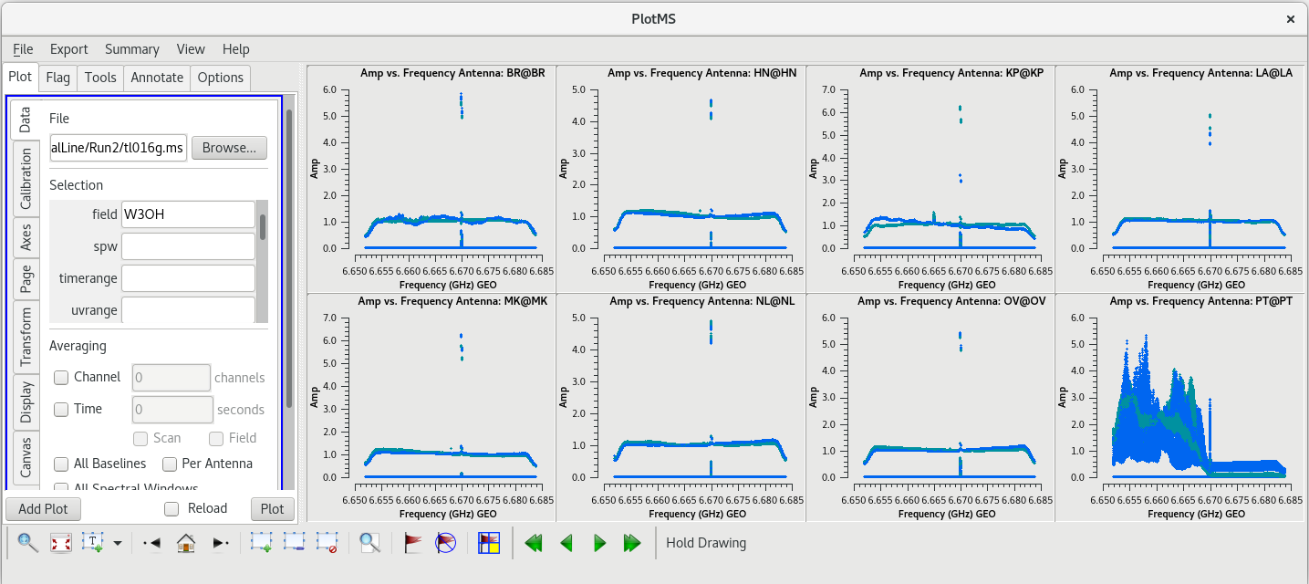
Because this observation was looking for a strong maser line, one of the first things we should do is check that an emission line was detected from our target source. We will do this by using plotms to plot amplitude vs frequency for the target source, W3OH. We will pick a single scan to plot because it will help plotms run faster. Looking at the tl016g_listobs.txt file we made above, we can see that W3OH was the target of scans 4, 6, 8, 10, 12, 14, etc. One of my favorite hockey players, Brendan Shanahan of the Detroit Red Wings, wore jersey number 14, so we'll use that scan. As an extra shortcut, we will plot all of the antennas simultaneously using the gridrows and gridcols parameters.
#In CASA
plotms(vis='tl016g.ms', xaxis='frequency', yaxis='amp', field='W3OH', scan='14', correlation='rr,ll', gridrows=2, gridcols=4, iteraxis='antenna', coloraxis='corr')
You can see that there is a bright line near the center of each plot, so we did detect the maser line we were looking for. However, something looks terribly wrong on the Pie Town antenna (lower right). It appears that Pie Town was suffering from major radio frequency interference (RFI) right near the maser line.
Taking a Deeper Look at Pie Town
Let's take a closer look at Pie Town to see how bad things really were. To start, let's see if the RFI was only present when observing W3OH. Take a look at the primary fringe finder, J0102+5824. This time, we'll want to look at multiple scans. There were four scans on J0102+5824: 1, 46, 91, and 136.
#In CASA
plotms(vis='tl016g.ms', xaxis='frequency', yaxis='amp', field='J0102+5824', correlation='rr,ll', gridrows=2, gridcols=2, iteraxis='scan', coloraxis='corr')
You should see that the RFI is present in each scan. This is bad news for us. Because the RFI is persistent and so close to the maser line, we will probably need to flag the Pie Town antenna. We were already missing Fort Davis and Saint Croix, so losing Pie Town will bring us down to only seven stations.
Before we lose all hope in Pie Town, let's see if the RFI is only on the autocorrelations or if it also impacts the cross correlations. To plot the cross correlations to Pie Town, we will use the antenna parameter in plotms.
#In CASA
plotms(vis='tl016g.ms', xaxis='frequency', yaxis='amp', field='J0102+5824', antenna='PT', correlation='rr,ll', gridrows=2, gridcols=2, iteraxis='scan', coloraxis='corr')
You can see that the RFI does indeed cause problems on the corss correlations, but not nearly as bad as on the autocorrelations. If you want to see just the PT autocorrelations, set antenna='PT&&&' in the plotms GUI and click "Plot".
Identifying a Good Reference Antenna
VLBA calibration makes use of a reference antenna: one antenna that all other antennas can be referenced to when generating solutions. Usually, you will want to use one of the more central stations: FD, KP, LA, or PT. For this observation, FD was missing (see the Observing Log), and we know PT had RFI issues. So, our choices are down to KP and LA.
To determine which is the best to use as the reference antenna, use plotms to plot phase vs frequency for a single scan on a bright source (usually the fringe finder or bandpass calibrator). For this observation, use the second scan on J0102+5824, which is scan 46 from the listobs output. We start with scan 46 because it is near the middle of our observation, so J0102+5824 should be at relatively high elevations at all stations during that scan. We will look at all the baselines to LA first.
#In CASA
plotms(vis='tl016g.ms', field='J0102+5824', xaxis='freq', yaxis='phase', scan='46', antenna='LA', correlation='rr,ll', gridrows=2, gridcols=4, iteraxis='baseline', coloraxis='corr')
Initially, this does not look very good. However, our observation used a lot of spectral channels. Averaging across spectral channels may make things look a bit nicer. In the GUI on the "Data" tab, look for the "Averaging" area. Check the box next to "Channel" and change "0" to "20" to average 20 spectral channels together for these plots. The plots using the averaged channels are much less noisy and look pretty good.
We should also look at our back-up fringe finder, J0217+7349, to see how it compares to J0102+5824. In the GUI, change the "Field" parameter to J0217+7349, and change the scan number to 47 (the second scan on J0217+7349), then click "Plot". Once the data for J0217+7349 appears, pay close attention to the LA-MK baseline. This baseline does not look as clean as it did for J0102+5824. This indicates that J0102+5824 is the better fringe finder and bandpass calibrator.
Now, we will check the baselines to KP. In the GUI, in the "Data" tab and under "Selection", change "field' back to "J0102+5824" and change "antenna" to "KP", then click plot. Comparing the LA and KP plots, both antennas look pretty good. Try plotting amplitude vs frequency for both antennas. In the GUI, under "Averaging", uncheck the box next to "Channels"; we want to look at all of the frequency channels again. Next, go to the "Axes" tab and change the "Data" axis from "Phase" to "Amp" and click "Plot". Once you have had a chance to look these over, go back to the "Data" tab and change the antenna back to LA.
Comparing the phase and amplitude plots for LA and KP, there is no clear advantage to using either antenna as the reference.
For spectral line observations, it is often a good idea to also inspect the autocorreltion data for signs of strong RFI at each site. You can plot the autocorrelations by setting the antenna parameter to *&&&.
#In CASA
plotms(vis='tl016g.ms', xaxis='frequency', yaxis='amp', field='J0102+5824', scan='46', correlation='rr,ll', gridrows=2, gridcols=4, antenna='*&&&', iteraxis='antenna', coloraxis='corr')
We already knew that PT had problems, but you should see that KP may have had issues with RFI as well.
For this observation, we will use Los Alamos (LA) as the reference antenna. Its phases are fairly smooth, it is free of RFI, and the bandpasses look pretty clean.
Identifying a Good Time Range for the Instrumental Delay Calibration
Next, we will look for a good time interval (about 1 minute long) for the instrumental delay calibration. This will be done using the fringe finder (J0102+5824), so we should inspect each scan on it: 1, 46, 91, and 136. We will want to plot amplitude vs time for each of these scans. To save time, we will just plot the baselines to the reference antenna, LA.
#In CASA
plotms(vis='tl016g.ms', xaxis='frequency', yaxis='amp', field='J0102+5824', antenna='LA', correlation='rr,ll', gridrows=2, gridcols=2, iteraxis='scan', coloraxis='corr')
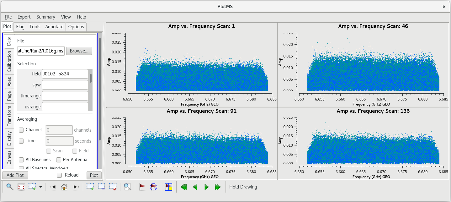 |
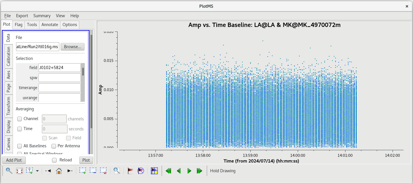 |
We probably want to avoid scans 1 and 136 since they are at the start and end of the observation, respectively. Scans 46 and 91 both look good. We have looked at scan 46 several times now, and have not noticed anything particularly bad on that, so we will use that scan. We should take a look at how the amplitude changes with time for scan 46. This time, it will be easier to look at each baseline separately and step through the plots interactively (you can try to plot them all at once, but you may find that the axes do not scale properly in each subplot).
#In CASA
plotms(vis='tl016g.ms', xaxis='time', yaxis='amp', field='J0102+5824', antenna='LA', scan='46', correlation='rr,ll', iteraxis='baseline', coloraxis='corr')
Step through each baseline to check for any problems. Things look pretty clean on each baseline. We will use one minute near the middle of the scan, 13:59:00 to 14:00:00, for our instrumental delay calibration
Flagging Data
In the VLBA Basic Phase-referencing tutorial, the first flagging step is to "quack" the date (flag the first and last few seconds of each scan). However, we did not notice any real problems at the begining or end of scan 46. So, we probably do not need to quack these data.
Flagging Problem Times
The first scan of VLBA observations often have some minor problems during the first few seconds. We should take a look at scan 1 to see if this observation has any such problems.
#In CASA
plotms(vis='tl016g.ms', xaxis='time', yaxis='amp', scan='1', antenna='LA', correlation='rr,ll', gridrows=2, gridcols=4, iteraxis='baseline', coloraxis='corr')
You should notice that there are low amplitude points during the first few seconds of the scan. We are going to want to flag these low points. Using the zoom tool in the GUI, you can identify the times that need to be flagged. We will flag the first 12 seconds of scan 1.
#In CASA
flagdata(vis='tl016g.ms', mode='manual', scan='1', timerange='12:31:00~12:31:12')
If you kept the plotms window open, you can check the "Reload" box and then click "Plot" to update the plots. You should see that the low points are now gone.
Flagging Problem Antennas
We know from our inspection of the fringe finders that PT has some major RFI near the maser line. Therefore, we should not include PT in our calibration. In fact, we should not use PT at all since it may be contributing bad data and/or noise to our observations.
Flag the PT antenna for the entire observation by using the flagdata command
#In CASA
flagdata(vis='tl016g.ms', mode='manual', antenna='PT')
Automated Flagging
The flagdata task includes a useful automated flagging mode known as "TFCrop". For more details on using the automated TFcrop mode, see the VLA CASA Flagging topical tutorial. Because this is a spectral line data set, we want to limit the automatic flagging to only the time domain. We will also avoid flagging on the maser lines, just to be extra careful (the maser lines are so bright that a small amount of RFI will not make any real difference).
To begin, you just want to get a feel for what TFCrop will do to the data, which means you should set action='calculate' .
#In CASA
flagdata(vis='tl016g.ms', mode='tfcrop', datacolumn='data', field='0,1,2', timecutoff=4.0, flagdimension='time', action='calculate', display='both')
This will open a new window with a GUI. The top row of the GUI will display the data as it currently is. The bottom row shows what the data will look like after the flags are applied (blue regions are flagged). Step through the antennas by clicking "Next Baseline". Step through at least a few scans by clicking "Next Scan". With timecutoff=4.0, it should really only flag those data points that are 4-times the standard deviation in the time dimension. This should be sufficient to remove the worst of the time-dependent RFI in our observation. For all of the baselines in the first scan, you will notice that there is a blue band at the bottom of the plots. This is the result of flagging the first 12 seconds of scan 1 above. Click on "Next Scan" to take a look at the data on J0217+7349. Stepping through the baselines on this scan, you should see that not much gets flagged. However, some very bright points are found and flagged by the code, which is exactly what we want to see. Take some time to look at some scans on the phase reference calibrator, J0306+6243, as well.
To generate the flags, we will need to run flagdata again with action='apply' .
#In CASA
flagdata(vis='tl016g.ms', mode='tfcrop', datacolumn='data', field='0,1,2', timecutoff=4.0, flagdimension='time', action='apply', display='both')
You should double check that the automatic flagging will behave as you expect. Once you are satisfied that the flagging will do what you want, click "Stop Display". The program will then look through the entire observation and apply the flags.
NOTE: You can always exit the TFCrop mode without applying any flags by clicking "Quit", even when you set action='apply' .
Flagging "By Hand"
As telescope arrays become larger and more complex, automated flagging will become the primary means of excluding bad data (just look at what ALMA does). However, the current VLBA is still small enough and the data rates are low enough that inspecting and flagging data oneself is not too painful.
You can look for obvious bad data using plotms. Be aware that while you can flag data in plotms, a major drawback to using plotms to flag data is that it makes undoing flags very difficult. The preferred method of flagging by hand is to identify the bad data with plotms, and then generate the flags with flagdata. It is recommended to be somewhat careful with flagging early on in the calibration process and only flag those data points that are obviously bad.
Let's start by taking a look at all the scans on our fringe finder and bandpass calibrator, J0102+5824. We will plot amplitude vs frequency for all four scans. We will aviod plotting the autocorrelations by setting antenna='*&*'
#In CASA
plotms(vis='tl016g.ms', xaxis='frequency', yaxis='amp', field='J0102+5824', correlation='rr,ll', antenna='*&*', gridrows=1, gridcols=4, iteraxis='scan', coloraxis='corr')
You should see that this looks pretty good. The final scan (136) may look a little low, but pay close attention to the y-axis values and you will notice that it is actually about the same as the other scans.
Now let's take a look at the phase reference calibrator. Again, we will plot amplitude vs frequency for all the scans. It will take a little longer to plot because there are so many more scans on this source.
#In CASA
plotms(vis='tl016g.ms', xaxis='frequency', yaxis='amp', field='J0306+6243', correlation='rr,ll', antenna='*&*', gridrows=2, gridcols=4, iteraxis='scan', coloraxis='corr')
Use the GUI to step through the plots. You should notice that scans 78 and 95 have spikes.
Let's take a closer look at scan 78 to narrow down where that bad data is coming from. We will start by plotting amplitude vs frequency, but iterate on the baselines.
#In CASA
plotms(vis='tl016g.ms', xaxis='frequency', yaxis='amp', field='J0306+6243', correlation='rr,ll', scan='78', antenna='*&*', gridrows=2, gridcols=4, iteraxis='baseline', coloraxis='corr')
Aha! The problem is isolated to the BR-OV baseline. Using the "Mark Regions" tool, draw a rectangle aruond the bad data, then click the "Locate" tool (the icon with the magnifying glass over a white rectangle). You should find that the bad data is limited to the time range 15:00:45 to 15:01:01. Plot amplitude vs time for scan 78 and limit the baseline to BR-OV.
#In CASA
plotms(vis='tl016g.ms', xaxis='time', yaxis='amp', field='J0306+6243', correlation='rr,ll', scan='78', antenna='BR&OV', coloraxis='corr')
You can see the bad data points are all above the value 0.015. Keep in mind that this is uncalibrated data, so the units on the Y axis don't really mean anything yet. We can get rid of these bad points by using mode='clip' in flagdata.
#In CASA
flagdata(vis='tl016g.ms', mode='clip', scan='78', clipminmax=[0.0, 0.015], clipoutside=True)
The combination of clipminmax=[0.0, 0.015] and clipoutside=True tells flagdata to flag anything with values outside of the range 0.0 to 0.015. If you kept the plotms window open, click "Reload" and the "Plot" to show the results of clipping the scan. You should see that all the bad data points are now gone, but the good data remains.
Now we will take a look at scan 95. Again, we will plot amplitude vs frequency for that scan and iterate on the baseline.
#In CASA
plotms(vis='tl016g.ms', xaxis='frequency', yaxis='amp', field='J0306+6243', correlation='rr,ll', scan='95', antenna='*&*', gridrows=2, gridcols=4, iteraxis='baseline', coloraxis='corr')
Using the GUI to step through the pages, you should notice that the spike is present on all baselines to KP. Let's take a look at amplitude vs time on KP for this scan.
#In CASA
plotms(vis='tl016g.ms', xaxis='time', yaxis='amp', field='J0306+6243', correlation='rr,ll', scan='95', antenna='KP', coloraxis='corr')
The bad data are not as obvious in this plot, and seem to cover the entire scan. If the bad data are not limited in time, they still appeared to be limited in frequency. In the GUI, go to the "Axes" tab and change the X-Axis to "Channel", then click "Plot. You should see that the bad data are indeed limited to a few spectral channels. Use the "Zoom" tool (the magnifying glass at the bottom left of the GUI) to select the region around the bad points. You should see that the bad data are limited to channels 258 to 262, so let's flag those channels on KP for this scan. To flag a select number of spectral channels, you need to use the spw parameter. In our case, set spw='0:258~262'. The 0 is for the spectral window (we only have the one in our data), and 258~262 tells flagdata to flag all channels in the ragne 258 to 262.
#In CASA
flagdata(vis='tl016g.ms', mode='manual', scan='95', antenna='KP', spw='0:258~262')
If your plotms window is still open, click "Reload" and "Plot" to show the impact of flagging the channels with the bad data.
These are the only major issues we spotted after the automated flagging, so now we will move on to the calibration.
Calibrating the Data
Earth Orientation Parameter Correction
When VLBI data are correlated, the correlator uses a model for where the Earth was in its rotation. Most of the time, that model is very good and the results are perfectly fine. Sometimes, however, the model is not quite good enough (e.g., a major earthquake happened in Hawaii during the time between when the model was made and when the observation occured, and the island moved a few millimeters). In these cases, it is important to make corrections for the inaccurate Earth orientation model.
NASA and others host sites that contain the most up-to-date Earth Orientation Parameters (EOP). You will need to retrieve the EOP from one of these hosts in order to make the EOP corrections to your data. To get the EOP file from NASA, use the curl command:
curl -u anonymous:<your-email-address> --ftp-ssl ftp://gdc.cddis.eosdis.nasa.gov/vlbi/gsfc/ancillary/solve_apriori/usno_finals.erp > /<path>/<to>/<file>/usno_finals.erp
You need to provide your email address (it serves as you password in the NASA system), and tell curl where to put the file. You should always put the EOP file in the same directory as the observation data. As an example, if your email address is "wade.wilson@marvelstate.edu" and you want the file in the file /home/user/mercwiththemouth/VLBA/SpectralLineTutorial/, you would enter the command:
curl -u anonymous:wade.wilson@marvelstate.edu --ftp-ssl ftp://gdc.cddis.eosdis.nasa.gov/vlbi/gsfc/ancillary/solve_apriori/usno_finals.erp > /home/user/mercwiththemouth/VLBA/SpectralLineTutorial/usno_finals.erp
You can keep the filename as "usno_finals.erp" or change it to something that makes sense to you. For this tutorial, we assume the filename is the default "usno_finals.erp".
Once you have the EOP file, you will create the EOP correction table using the gencal task.
#In CASA
gencal(vis='tl016g.ms', caltable='tl016g.eop', caltype='eop', infile='usno_finals.erp')
This will create the file "tl016g.eop" that contains the EOP calibration table.
You should check that the EOP values make sense by plotting them with plotms.
#In CASA
plotms(vis='tl016g.eop', xaxis='time', yaxis='phase', gridrows=2, gridcols=4, iteraxis='antenna', coloraxis='field')
For each target (field), the phases should be nice and smooth and the values should be small (about 10 degrees or less). Also check the delays and rates by going to the "Axes" tab in the GUI and changing the Y Axis to "delay" and "delay-rate", and clicking on "Plot". These should also be smooth with time and the values should be small.
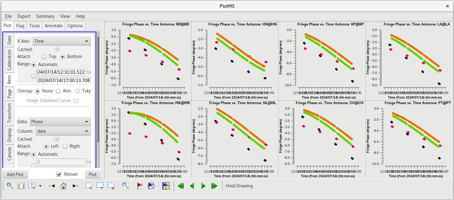 |
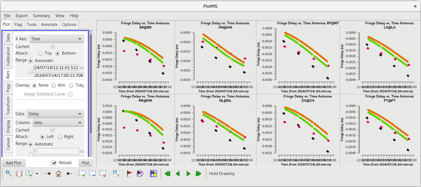 |
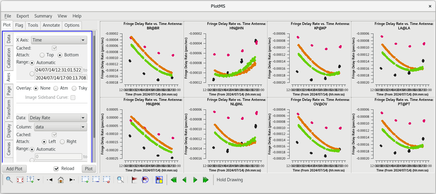 |
All of our EOP corrections look good.
Amplitude Corrections from Autocorrelations
Determine the amplitude corrections from the autocorrelations with accor. This corrects for errors introduced by the 2-bit sampling at the VLBA.
#In CASA
accor(vis='tl016g.ms', caltable='tl016g.accor', solint='30s', gaintable=['tl016g.eop'], interp=['nearest'])
NOTE: This step is not required for EVN data, because the EVN correlator performs it during correlation.
Inspect the tl016g.accor solution table with plotms.
#In CASA
plotms(vis='tl016g.accor', xaxis='time', yaxis='amp', gridrows=2, gridcols=4, iteraxis='antenna', coloraxis='corr')
Ideally, all of the solutions should be very close to 1.0. Looking through the solutions, you can see that everything is close to 1, but the solutions look a bit noisy.
The AIPS VLBA utility script VLBACCOR smooths the autocorrelation corrections by default (with a smoothing time of 30 minutes). It is possible to do this smoothing in CASA 6.3 and later using the smoothcal task. Based on what we saw in our plotting, these data would likely benefit from some smoothing.
#In CASA
smoothcal(vis='tl016g.ms', tablein='tl016bg.accor', caltable='tl016g_smooth.accor', smoothtype='median', smoothtime=1800.0)
Remember to check the smoothed solutions with plotms to make sure it was an improvement.
#In CASA
plotms(vis='tl016g_smooth.accor', xaxis='time', yaxis='amp', gridrows=2, gridcols=4, iteraxis='antenna', coloraxis='corr')
The smoothed solutions look a bit better. The only odd antenna is LA, but even those solutions are all close to 1 and look pretty smooth.
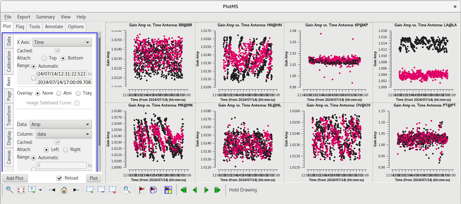 |
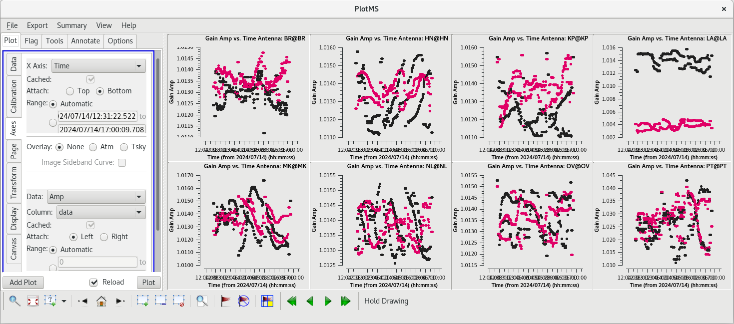 |
A Priori Calibration
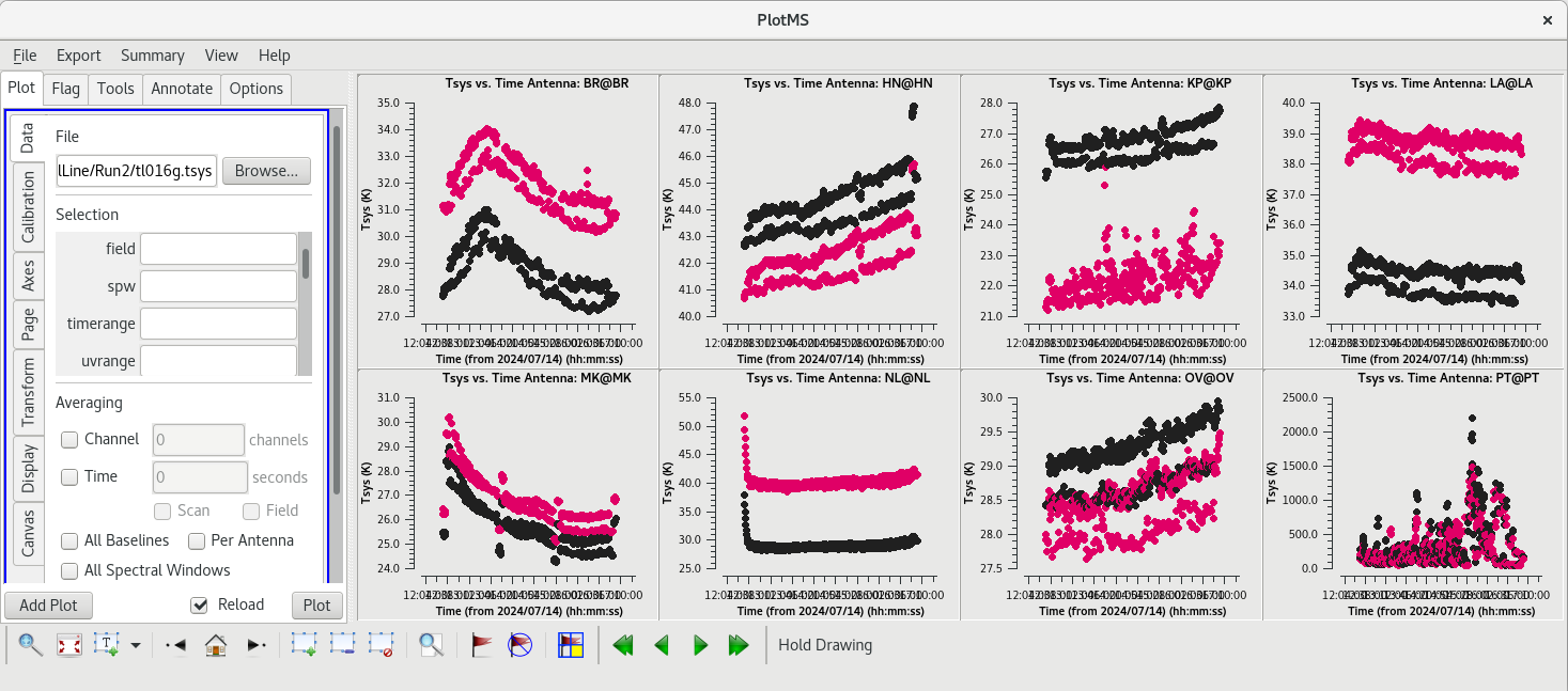
Unlike the VLA, the VLBA cannot rely on bootstrapping absolute flux density calibration from a well-modeled calibrator. Instead, the VLBA relies on a combination of the system temperature and the known gain curve of the antennas (how the gain of the antenna changes with elevation). Both the system temperatures and gain curves are included in the FITS-IDI file, and both are imported into the Measurement Set with importfitsidi. To get the system temperature and gain curve information into a form that CASA can use for calibration, we use the gencal task to generate calibration tables.
System temperature:
gencal(vis='tl016g.ms', caltable='tl016g.tsys', caltype='tsys', uniform=False)
Check the system temperature table with plotms.
#In CASA
plotms(vis='tl016g.tsys', xaxis='time', yaxis='tsys', iteraxis='antenna', coloraxis='corr')
The system temperature values mostly look good. They vary smoothly at most stations, and the values are reasonable for C-band (between about 20 and 50 K). Notice that you cannot really tell the difference between scans on maser and scans on calibrators. Even though the maser lines are incredibly bright, they are so narrow that they do not impact the system temperatures much. There is some weird behavior on NL during the earliest scans, but the values are not too high. There are major problems on PT, however. That broadband RFI that we noticed earlier caused the system temperature values for that station to be very high and messy. If we had not already flagged the PT antenna, we would definitely do it now.
Gain curve:
#In CASA
gencal(vis='tl016g.ms', caltable='tl016g.gcal', caltype='gc')
This observation was done at 6.7 GHz and with a bandwidth of only 32 MHz. The gain curve is very uninteresting, so we will not bother looking at the solutions now (although you can if you really want to). If your observation is at 12 GHz or higher, you will probably want to inspect the gain curve table with plotms.
NOTE: For EVN observations, the system temperatures and gain curves are provided in ANTAB files rather than in the FITS-IDI file. If you are working with EVN data, you must append the system temperature data to the FITS-IDI file before running importfitsidi. EVN gain curves must also be extracted from the ANTAB file. For more information, see the EVN Data Reduction Guide.
Instrumental Delay Calibration
Solve for the instrumental delays by using fringefit on a bright source (the "fringe finder"). In our case, the fringe finder is J0102+5824. Set the timerange to the one-minute time span you identified while inspecting the data earlier. Because we are only solving for the instrumental delays (changes in phase as a function of frequency), we will set zerorates=True to set all of the delay-rates (changes in phase as a function of time) to be zero.
#In CASA
fringefit(vis='tl016g.ms', caltable='tl016g.sbd', field='J0102+5824', timerange='13:59:00~14:00:00', solint='inf', zerorates=True, refant='LA', minsnr=10, gaintable=['tl016g.eop', 'tl016g_smooth.accor', 'tl016g.gcal', 'tl016g.tsys'], interp=['nearest', 'nearest', 'nearest', 'nearest,nearest'], parang=True)
Notice that we are pre-applying the EOP, sampling corrections, gain curve, and system temperature when we run fringefit. We are also applying the parallactic angle correction (parang=True), which is necessary to do prior to any phase referencing.
Watch the logger for any reports of low SNR and failures to converge on a solution. Ideally, the SNR for each station should be very high (for our data, all reported SNR values are larger than 380, which is pretty good).
A Note on Table Names: In the Basic Phase-referencing tutorial, we followed the convention of naming tables as described in the EVN CASA tutorials. The instrumental delay table was called "sbd", which stood for "single band delay". It is not necessary to follow this convention. You can name a calibration table anything you want. For example, you could set caltable='tl106g.instdly' for the instrumental delay. Just be sure to keep track of your tables and to apply them appropriately in the calibration tasks.
Once fringefit has finished, you should see the following in the logger:
Finished solving.
Calibration solve statistics per spw:  (expected/attempted/succeeded):
  Spw 0: 1/1/1
This is exactly what we expect to see. We are only attempting to get one solution per spw because we are only solving over a single solution interval (one minute of data from a single scan).
Apply the instrumental delay corrections using applycal.
#In CASA
applycal(vis='tl016g.ms', gaintable=['tl016g.eop', 'tl016g_smooth.accor', 'tl016g.gcal', 'tl016g.tsys', 'tl016g.sbd'], interp=['nearest', 'nearest', 'nearest', 'nearest,nearest', 'nearest'], parang=True)
NOTE: In applycal, the order in which you specify the list for gaintable sets the order for both interp and spwmap. If you change the order of gaintable, be sure to also change the order of interp and spwmap! Also, if you smoothed any of the solutions, be sure to use the appropriate filename for the smoothed table.
It may take a little while (~2 minutes or more) for applycal to finish. If you are watching the logger carefully, you will see the message "Adding CORRECTED_DATA column(s)". Because this is the first time that we have run applycal, CASA needs to create a new column containing the data with the corrections applied.
Check that applying the solutions resulted in improvements:
#In CASA
plotms(vis='tl016g.ms', field='J0102+5824', xaxis='frequency', yaxis='phase', ydatacolumn='corrected', timerange='13:59:00~14:00:00', correlation='rr,ll', antenna='*&*', gridrows=2, gridcols=4, iteraxis='antenna', coloraxis='antenna2')
Ideally, the phase values should now be clustered around 0 degrees. For our data, all of the plots are nicely centered on 0 degrees, but there is a lot of scatter because of the large number of spectral channels. To make things a little easier to look at, we will average 20 spectral channels like we did when we were looking for a good reference antenna (in the "Data" tab, under "Averaging", check the box next to "Channels" and change the value to 20, then click "Plot"). The averaged plots should have much less scatter in the phases.
Global Fringe Fitting
Now, we will solve for the time and frequency-dependent effects in phase using fringefit, also known as "global fringe fitting" (or sometimes "multi-band delay", if you have multiple spectral windows and you combine them during this step). We will need to pick a solution interval that is appropriate for our data. It should be at least 10 seconds, and no longer than the scan length on the phase reference calibrator. For this observation, we will need to use solint='inf', which will give one solution for each scan on the calibrator sources.
NOTE: You are welcome to try a shorter solution interval, but you will probably run into a problem where there is a tiny bit of a scan left after the solution interval and fringefit will fail.
For refant, enter a list of antennas to try as the reference antenna. The preferred refant should be listed first, followed by the second choice, then third choice, and so on. It is not recommended to include Mauna Kea (MK) or Saint Croix (SC) in the list, unless the phase reference calibrator is very bright on the longest baselines. BR and HN are often omitted for the same reason. For our observation, we will set the list to LA, KP, OV, and NL. Set field to the fringe finder, the backup fringe finder, and the phase reference calibrator.
#In CASA
fringefit(vis='tl016g.ms', caltable='tl016g.mbd', field='J0102+5824, J0217+7349, J0306+6243', solint='inf', minsnr=5, zerorates=False, refant='LA,KP,OV,NL', gaintable=['tl016g.eop', 'tl016g_smooth.accor', 'tl016g.gcal', 'tl016g.tsys', 'tl016g.sbd'], interp=['nearest', 'nearest', 'nearest', 'nearest,nearest', 'nearest'], parang=True)
This step may take quite a while (probably at least 20 minutes), so this is a good opportunity to stand up, stretch, and go get a tasty beverage.
When the fringefit task is done, check the logger for the solution statistics ("expected/attempted/succeeded"). You want all three numbers to be the same, or at least very similar.
For our project, you should see something like this in the logger:
Finished solving.
Calibration solve statistics per spw:  (expected/attempted/succeeded):
  Spw 0: 74/74/74
Because fringefit ran successfully and we are satisfied that the number of solutions is appropriate, we should now take a look at the solutions with plotms.
#In CASA
plotms(vis='tl016g.mbd', xaxis='time', yaxis='phase', gridrows=2, gridcols=4, iteraxis='antenna', coloraxis='corr')
Use the GUI to switch the yaxis between 'Phase', 'Delay', and 'Delay Rate'. The phase and delay solutions should both vary smoothly with time. If they do not, you may need to smooth the table before applying it. The delay-rates should be clustered around zero with some scatter. You should see that the solutions on all antennas look pretty good.
Now that we are confident that the global fringefit solutions are good, we will apply them with applycal.
#In CASA
applycal(vis='tl016g.ms', gaintable=['tl016g.eop', 'tl016g_smooth.accor', 'tl016g.gcal', 'tl016g.tsys', 'tl016g.sbd', 'tl016g.mbd'], interp=['nearest', 'nearest', 'nearest', 'nearest,nearest', 'nearest', 'linear'], parang=True)
It will probably take a while (about 2 minutes) for applycal to run this time.
Take a look at the data with plotms to make sure the corrections are improving the phases. We'll look at the back up fringe finder, J0217+7349. We'll start by looking at the uncalibrated phases. We will average the data in the time dimension, using a 60-second average time, to be able to see the details.
#In CASA
plotms(vis='tl016g.ms', xaxis='frequency', yaxis='phase', ydatacolumn='data', field='J0217+7349', antenna='*&*', scan='92', correlation='rr,ll', gridrows=2, gridcols=4, iteraxis='antenna', coloraxis='corr', avgtime='60')
The uncalibrated data is pretty much a mess. Now, go to the "Axes" tab and change the Data Column from "data" to "corrected". The corrected data should look much better, with the phases centered around zero degrees with some scatter.
Bandpass Calibration
Now we will correct for the shape of the bandpass using the bandpass task. This step requires a very bright source (perferably >1 Jy on all baselines), so we will use our fringe finder J0102+5824. However, unlike when we solved for the instrumental delay (above), we will use all of the scans on the source.
#In CASA
bandpass(vis='tl016g.ms', caltable='tl016g.bpass', field='J0102+5824', solint='inf', refant='LA', solnorm=True, bandtype='B', gaintable=['tl016g.eop', 'tl016g_smooth.accor', 'tl016g.gcal', 'tl016g.tsys', 'tl016g.sbd', 'tl016g.mbd'], interp=['nearest', 'nearest', 'nearest', 'nearest,nearest', 'nearest', 'linear'], parang=True)
Inspect the solutions with plotms.
#In CASA
plotms(vis='tl016g.bpass', xaxis='frequency', yaxis='amp', gridrows=2, gridcols=4, iteraxis='antenna', coloraxis='corr')
The amplitude corrections should be near 1. For spectral line obsevrations, the bandpass solutions need to be very smooth. If you notice any outliers, you delete that table, go back to the data and look carefully for any outliers that may have led to poor bandpass solutions and flag them. Then run the bandpass calibration again and check that the solutions look better. While looking over the solutions, also make sure to check the phases (uses the GUI to set yaxis='phase'). You should see that the phase solutions are all near zero degrees.
Apply the solutions with applycal.
#In CASA
applycal(vis='tl016g.ms', gaintable=['tl016g.eop', 'tl016g_smooth.accor', 'tl016g.gcal', 'tl016g.tsys', 'tl016g.sbd', 'tl016g.mbd', 'tl016g.bpass'], interp=['nearest', 'nearest', 'nearest', 'nearest,nearest', 'nearest', 'linear', 'linear,linear'], parang=True)
It will probably take a while for applycal to run again, since you are also applying the solutions from the global fringe fitting.
After applying the bandpass solutions, take a look at the calibrated data with plotms.
#In CASA
plotms(vis='tl016g.ms', xaxis='frequency', yaxis='amp', ydatacolumn='corrected', field='J0102+5824', antenna='*&*', correlation='rr,ll', gridrows=2, gridcols=4, iteraxis='baseline', coloraxis='corr')
You should see that the edges of the spectral window are higher than the rest of the channels. We will flag the first and last ten channels to get rid of these high points.
#In CASA
flagdata(vis='tl016g.ms', spw='0:0~10;630~639')
If you kep your plotms window open, check the "Reload" box and click "Plot" to show the effect of flagging the edge channels. You should see that all of the antennas show a nice, flat bandpass.
In the Basic Phase-referencing tutorial, the next step was to do a final amplitude calibration. However, that step is only necessary for data with bandwidths of 256 MHz or larger. That definitely is not the case for this project, so we will skip that step. (It should not hurt to do it, it just is not necessary.)
Also, in the Basic Phase-referencing tutorial, we split the calibrated data at this point and performed self-calibration on the split file. For this tutorial, we will continue with self-calibration using the orignal data MS. The reason for this will become obvious soon. (Students are encouraged to think about why that might be and see if they are correct later!)
However, we will use split to save our progress, just in case we make any mistakes after this point.
NOTE: The split step is optional, and just a precaution in case we ake mistakes later. This will create a new 4 GB MS file on your disk. If you are very low on disk space, you may want to skip this step, or set the outputvis parameter such that it writes the new MS to an external drive.
#In CASA
split(vis='tl016g.ms', outputvis='tl016g_initialcal.ms', antenna='*&*', datacolumn='all')
Notice that we are not bothering to save the autocorrelations (we do not need them anymore after running accor). Setting datacolumn='all' makes sure we keep both the uncalibrated data and the calibrated data.
We are now done with the initial calibration.
Self-Calibration of Phase Reference Calibrator
Despite our best efforts with the initial calibration, VLBA observations will almost always require additional steps to improve the calibration. Because the VLBA antennas are separated by such large distances, the phases may not be perfectly calibrated by fringe fitting alone. This is partly because each antenna may be looking through vastly different troposphere/ionosphere, and partly because the phase reference calibrators are rarely point sources on long baselines (and fringe-fitting usually assumes the calibrators are point sources on all baselines).
We will improve the calibration using "self-calibration". The process of self-calibration involves building models of the sources, refining the calibration based on those models, and then repeating until you converge to a good solution. The models are created during the imaging process. Each iteration of self-calibration should produce images with lower noise.
More details on self-calibration can be found in the Basic Phase-referencing tutorial. This tutorial will only cover the steps.
Imaging the Phase Reference Calibrator
To create images of our sources, we will use tclean.
#In CASA
tclean(vis='tl016g.ms', field='J0306+6243', imagename='J0306_sc1', imsize=[320], cell=['0.2mas'], stokes='I', deconvolver='clark', weighting='natural', niter=1000, interactive=True, savemodel='modelcolumn')
Setting interactive=True will allow us to define the areas where there is real flux from the source ("clean windows"). The value for niter needs to be large enough that we can go through enough clean iterations to recover most of the source flux. You can set niter to any arbitrarily large number (a few hundred should be plenty), but 1000 is an easy value to remember. Setting savemodel='modelcolumn' will save the model we create for the image to the model column of the measurement set so we can use it for self-calibration.
Running tclean with interactive=True will open a new Viewer Display Panel where you can control the cleaning of the image. You should see that J0306+6243 is fairly point-like. Use the zoom tool to select the region around the source. Use the "polygon drawing" tool to draw a clean window around the source, excluding the stuff to the left and right of the bright source. Click on the "Continue deconvolution" button (the green circular arrow on the right). Check the residuals when the display updates. Stop cleaning when the area around the source looks noise-like. For example, if you notice positive and negative regions with similar magnitudes (e.g., +0.003 and -0.003) inside your clean window, that is probably a good time to stop cleaning. To stop the cleaning process, click the "stop deconvolving now" button (the red circle with the white "X"). It may take tclean a while to finish and close.
NOTE: If you need to delete a clean window, select "Erase" at the far left of the green region in the GUI and draw a box around the clean window(s) you want to delete, then double click. Remember to select "Add" again to define new clean windows.
Tracking Improvement
To ensure that self-calibration is actually helping to improve the quality of the images, you should track some image statistics. The most reliable way to do this is to define 2 boxes in the image; one box that contains the source ("on-source"), and one box that does not contain any part of the source ("off-source"). You can use imview to inspect the image and determine where to place the on-source and off-source boxes.
#In CASA
imview
In the GUI, go to Data->Open->J1154_sc1.image, then click "raster image" to load the image we just created. Use the zoom tool to select the area around the source. Use the "rectangle drawing" tool to create a box around the source and record the pixel locations of the lower left and upper right corners. The on-source box should be fairly small and fit tightly around the source. For example, lower left = [150, 135], upper right = [175,185] looks like it should work. Now, zoom out and draw another box somewhere off the source. You can make the off-source box pretty big. For example, lower left = [18,236], upper right = [299,305]. To make things a little easier, we will assign the values of our on- and off-source boxes to some variables in CASA:
#In CASA
j0306_onbox = '150,135,175,185'
j0306_offbox= '18,236,299,305'
Once you have your on- and off-source boxes defined, use the task imstat to gather some statistics about those regions.
#In CASA
imstat(imagename='J0306_sc1.image', box=j0306_onbox)
imstat(imagename='J0306_sc1.image', box=j0306_offbox)
Running imstat will return several values in both the logger and the CASA terminal. The values of interest for the self-calibration process are the on-source peak value ("max"), the on-source total flux density ("flux"), and the off-source RMS value ("rms"). It is a very good idea to record each of these values for each image (including the first image without any self-calibration applied) as you proceed with self-calibration. Ideally, the on-source peak and total flux values will increase slightly and the off-source RMS will decrease significantly as you improve the calibration. However, be very suspicious of large increases (>10%) in flux density values, especially when the off-source RMS does not improve dramatically.
For the first image of J0306+6243, the values should be fairly close to:
On-source:
'flux': 0.167
'max': 0.172
Off-source:
'rms': 0.00059
This is a signal-to-noise ratio of about 280, which is pretty good. Record these values in your notes so you have a way to check if self-calibration is leading to improvements in the images.
Phase Self-Calibration
Now that we have an initial model of the phase reference calibrator (from the image), we can begin the self-calibration process. In CASA, this is done with the gaincal task.
NOTE: In the Basic Phase-referencing tutorial, we performed the self-calibration steps on the split dataset. In this tutorial, we are using the initial dataset (for reasons that will become obvious later). Therefore, we must remember to pre-apply all of the calibration tables during our self-calibration steps.
We will start with refining the delays using our image of J0302+6243.
#In CASA
gaincal(vis='tl016g.ms', field='J0306+6243', caltable='tl016g.dcal', solint='inf', refant='LA', minblperant=3, gaintype='K', calmode='p', gaintable=['tl016g.eop', 'tl016g_smooth.accor', 'tl016g.gcal', 'tl016g.tsys', 'tl016g.sbd', 'tl016g.mbd', 'tl016g.bpass'], interp=['nearest', 'nearest', 'nearest', 'nearest,nearest', 'nearest', 'linear', 'linear,linear'], parang=True)
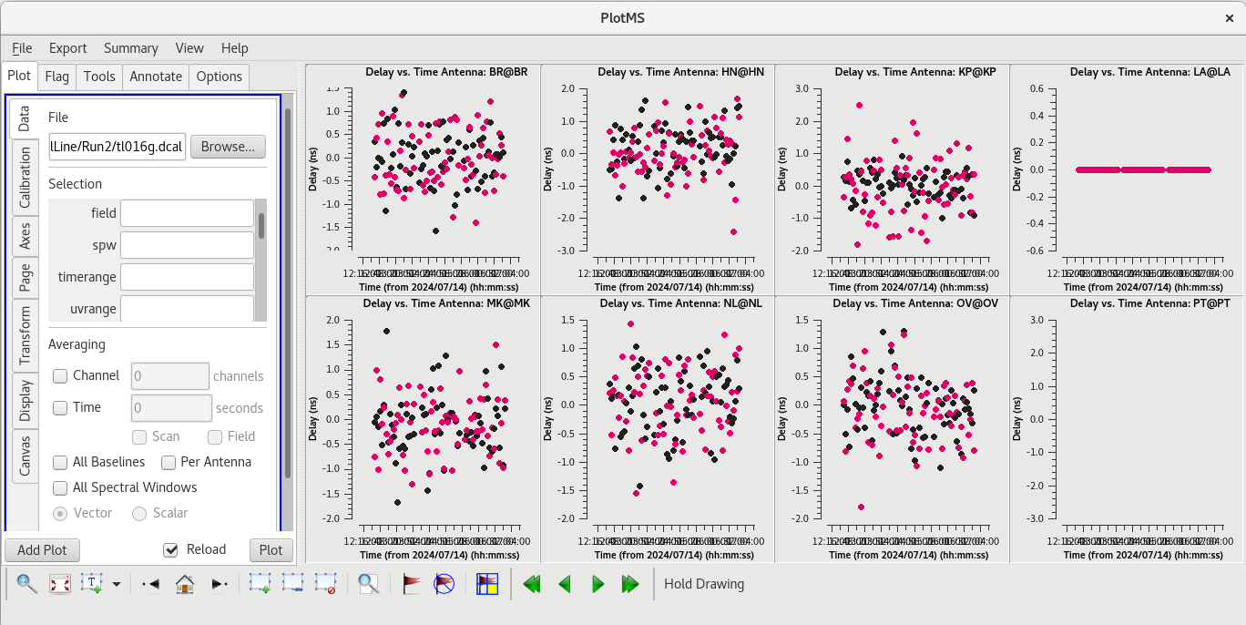
When gaincal finishes, check the logger window. You should see:
Finished solving.
Calibration solve statistics per spw:  (expected/attempted/succeeded):
  Spw 0: 66/66/66
CASA found 66 solution intervals based on our solint, it attempted to find a solution for all 66 intervals, and it succeeded on all 66 attempts. This is what we want to see. Plot the delay solutions and inspect them.
#In CASA
plotms(vis='tl016g.dcal', xaxis='time', yaxis='delay', gridrows=2, gridcols=4, iteraxis='antenna', coloraxis='corr')
You should see that the solutions are all small (a few nanoseconds) and centered around zero.
Next, we will refine the phases. For this step, we will set the solution interval to 20 seconds (solint='20s' ) to give us two solutions per scan on the phase reference calibrator.
#In CASA
gaincal(vis='tl016g.ms', field='J0306+6243', caltable='tl016g.pcal', solint='20s', refant='LA', minblperant=3, gaintype='G', calmode='p', gaintable=['tl016g.eop', 'tl016g_smooth.accor', 'tl016g.gcal', 'tl016g.tsys', 'tl016g.sbd', 'tl016g.mbd', 'tl016g.bpass', 'tl016g.dcal'], interp=['nearest', 'nearest', 'nearest', 'nearest,nearest', 'nearest', 'linear', 'linear,linear', 'linear'], parang=True)
Note that we are pye-applying all of the initial calibration and the refined delays when we do the phase self-calibration.
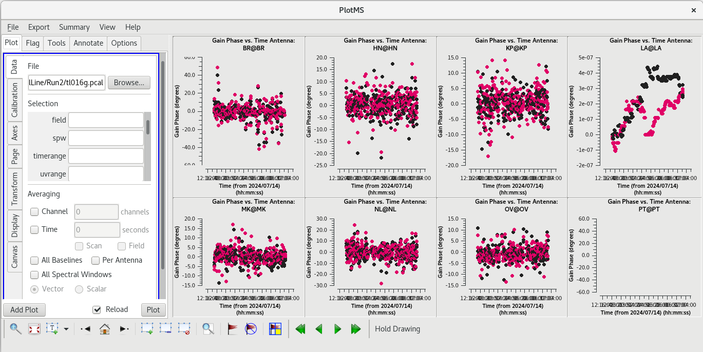
Checking the logger, you should see:
Finished solving.
Calibration solve statistics per spw:  (expected/attempted/succeeded):
  Spw 0: 263/263/263
Again, all the of the numbers match, which is what we want to see.
Inspect the phase solution table with plotms.
#In CASA
plotms(vis='tl016g.pcal', xaxis='time', yaxis='phase', gridrows=2, gridcols=4, iteraxis='antenna', coloraxis='corr')
As with the delays, all of the solutions should be clustered around zero. Most of the antennas look very good. BR has a few mildly concerning outliers, but nothing outrageous.
Notice that when refining both the delays and the phases we set minblperant=3 because closure phases require at least 3 baselines.
Apply the phase self-calibration solutions to the phase reference calibrator.
#In CASA
applycal(vis='tl016g.ms', gaintable=['tl016g.eop', 'tl016g_smooth.accor', 'tl016g.gcal', 'tl016g.tsys', 'tl016g.sbd', 'tl016g.mbd', 'tl016g.bpass', 'tl016g.dcal', 'tl016g.pcal'], interp=['nearest', 'nearest', 'nearest', 'nearest,nearest', 'nearest', 'linear', 'linear,linear', 'linear', 'linear'], parang=True)
Make a new image after the improved phase calibration using tclean just as we did previously. Remember to use a new imagename for this new image of the phase self-calibrated data.
#In CASA
tclean(vis='tl016g.ms', field='J0306+6243', imagename='J0306_sc2', imsize=[320], cell=['0.2mas'], stokes='I', deconvolver='clark', weighting='natural', niter=1000, interactive=True, savemodel='modelcolumn')
Once you have created the new image, check for improvement with imstat. As long as you did not change the imsize or cell parameters, you can use the same on- and off-source boxes that we defined earlier.
#In CASA
imstat(imagename='J0306_sc2.image', box=j0306_onbox)
imstat(imagename='J0306_sc2.image', box=j0306_offbox)
For the second image of J0306+6243, the values should be fairly close to:
On-source:
'flux': 0.167
'max': 0.172
Off-source:
'rms': 0.00057
Record these values in your notes. There is a small improvement in the rms, but the amount of cleaned flux remains almost exactly the same.
Amplitude Self-Calibration
#In CASA
gaincal(vis='tl016g.ms', field='J0306+6243', caltable='tl016g.apcal', solint='inf', refant='LA', minblperant=4, gaintype='G', calmode='ap', solnorm=True, gaintable=['tl016g.eop', 'tl016g_smooth.accor', 'tl016g.gcal', 'tl016g.tsys', 'tl016g.sbd', 'tl016g.mbd', 'tl016g.bpass', 'tl016g.dcal', 'tl016g.pcal'], interp=['nearest', 'nearest', 'nearest', 'nearest,nearest', 'nearest', 'linear', 'linear,linear', 'linear', 'linear'], parang=True)
Notice that we have set minblperant=4 because closure amplitudes require 4 baselines, and solint='inf' to use the full scan for each solution.
In the logger, you should see:
Finished solving.
Calibration solve statistics per spw:  (expected/attempted/succeeded):
  Spw 0: 66/66/66
All of the numbers match, which is what we like to see. Scrolling up a little in the logger, you should find a line that says something like "Normalization factor (MEAN) for spw 0 = 1.01489". Typically, you want this average normalization factor to be close to 1.0, indicating that none of the antennas had a major flux density scaling problem. Ours is about 1.015, which is a good result.
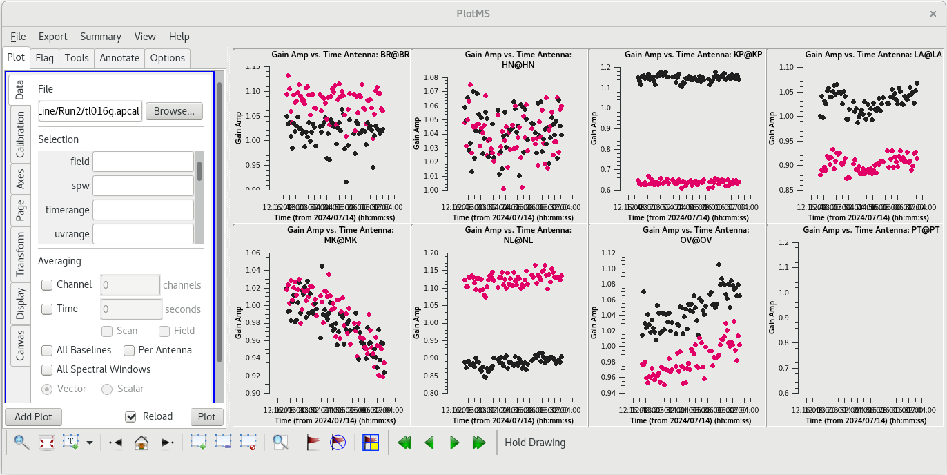
We should take a look at the solutions on each telescope using plotms.
#In CASA
plotms(vis='tl016g.apcal', xaxis='time', yaxis='amp', gridrows=2, gridcols=4, iteraxis='antenna', coloraxis='corr')
You should see that most of the solutions are near 1.0, but a few telescopes have larger corrections. KP, LA, and NL show significant differences between the RR and LL data. This is not uncommon for VLBA observations, and the corrections are not suspiciously large.
Apply the amplitude solutions to the phase reference calibrator.
#In CASA
applycal(vis='tl016g.ms', gaintable=['tl016g.eop', 'tl016g_smooth.accor', 'tl016g.gcal', 'tl016g.tsys', 'tl016g.sbd', 'tl016g.mbd', 'tl016g.bpass', 'tl016g.dcal', 'tl016g.pcal', 'tl016g.apcal'], interp=['nearest', 'nearest', 'nearest', 'nearest,nearest', 'nearest', 'linear', 'linear,linear', 'linear', 'linear', 'linear'], parang=True)
Make one last image of the phase reference calibrator, just to check for improvements. Since we will not be doing any more self-calibration on this source, we will set savemodel='none' to save some time and disk space. Remember to use a new imagename again.
#In CASA
tclean(vis='tl016g.ms', field='J0306+6243', imagename='J0306_sc3', imsize=[320], cell=['0.2mas'], stokes='I', deconvolver='clark', weighting='natural', niter=1000, interactive=True, savemodel='none')
Check the image statistics to make sure the self-calibration is making an improvement
#In CASA
imstat(imagename='J0306_sc3.image', box=j0306_onbox)
imstat(imagename='J0306_sc3.image', box=j0306_offbox)
For the final image of J0306+6243, the values should be fairly close to:
On-source:
'flux': 0.189
'max': 0.177
Off-source:
'rms': 0.00023
This is a significant improvement over the phase self-calibrated image!
We are now done with the self-calibration of the data.
The Zoom Band Data
Next, we will load in the data where we have zoomed in on the maser lines. These data have much higher spectral resolution than the full data set.
# In CASA
importfitsidi(fitsidifile='TL016GZOOM.IDIFITS', vis='tl016g_zoom.ms', constobsid=True, scanreindexgap_s=15)
The first thing we want to do with the zoom band data is get rid of the PT station.
#In CASA
flagdata(vis='tl016g_zoom.ms', mode='manual', antenna='PT')
Now that we have a zoom band MS, we will apply all of the solutions we drived from the full data set to the zoom band data.
#In CASA
applycal(vis='tl016g_zoom.ms', gaintable=['tl016g.eop', 'tl016g_smooth.accor', 'tl016g.gcal', 'tl016g.tsys', 'tl016g.sbd', 'tl016g.mbd', 'tl016g.bpass', 'tl016g.dcal', 'tl016g.pcal', 'tl016g.apcal'], interp=['nearest', 'nearest', 'nearest', 'nearest,nearest', 'nearest', 'linear', 'linear,linear', 'linear', 'linear', 'linear'], parang=True)
It should now be clear why we did not do the self-calibration steps on the file we split out earlier. We wanted all of the calibration tables to come from the primary MS so we could safely apply them to the zoom MS.
We should inspect some of the data to make sure the calibration was applied properly. We'll start with looking at the phase vs frequency for one scan on the back up fringe finder, J0217+7349, just like we did after the global fringe fit step. Remember that we needed to average the data in time to see the details properly. Because we have so many spectral channels in our zoom band, it will be useful to also average in frequency for this plot.
#In CASA
plotms(vis='tl016g_zoom.ms', xaxis='frequency', yaxis='phase', ydatacolumn='corrected', field='J0217+7349', antenna='*&*', scan='92', correlation='rr,ll', gridrows=2, gridcols=4, iteraxis='antenna', coloraxis='corr', avgchannel='60', avgtime='60')
The phases are mostly centered around zero degrees, which is what we want to see. Let's take a look at more of the data and in a different way. We will plot the phases vs uv-distance (in unit of wavelength) for all scans on J0217+7349. For this plot, we will want to average even more of our spectral channels together.
#In CASA
plotms(vis='tl016g_zoom.ms', xaxis='uvwave', yaxis='phase', ydatacolumn='corrected', field='J0217+7349', antenna='*&*', correlation='rr,ll', coloraxis='corr', avgchannel='600', avgtime='60')
Again, the phases are generally centered around zero degrees. Things look like they get a little messy at the longer baselines, but this could be due to source structure. Overall, the calibrated data look pretty good.
Now that we are satisfied the calibration is good, we can start making images of the maser lines.
First, we will split out the calibrated data on our target, W3OH.
#In CASA
split(vis='tl016g_zoom.ms', outputvis='w3oh_zoom.ms', field='W3OH', antenna='*&*', datacolumn='corrected')
This will make a new MS which is about 2.8 GB in size. It will contain only W3OH, only the calibrated data, and only the cross-correlations.
Let's take a look at the spectrum for our zoom band data on the maser lines.
#In CASA
plotms(vis='tl016g_zoom.ms', field='W3OH', scan='87', xaxis='frequency', yaxis='amp', coloraxis='corr', iteraxis='antenna')
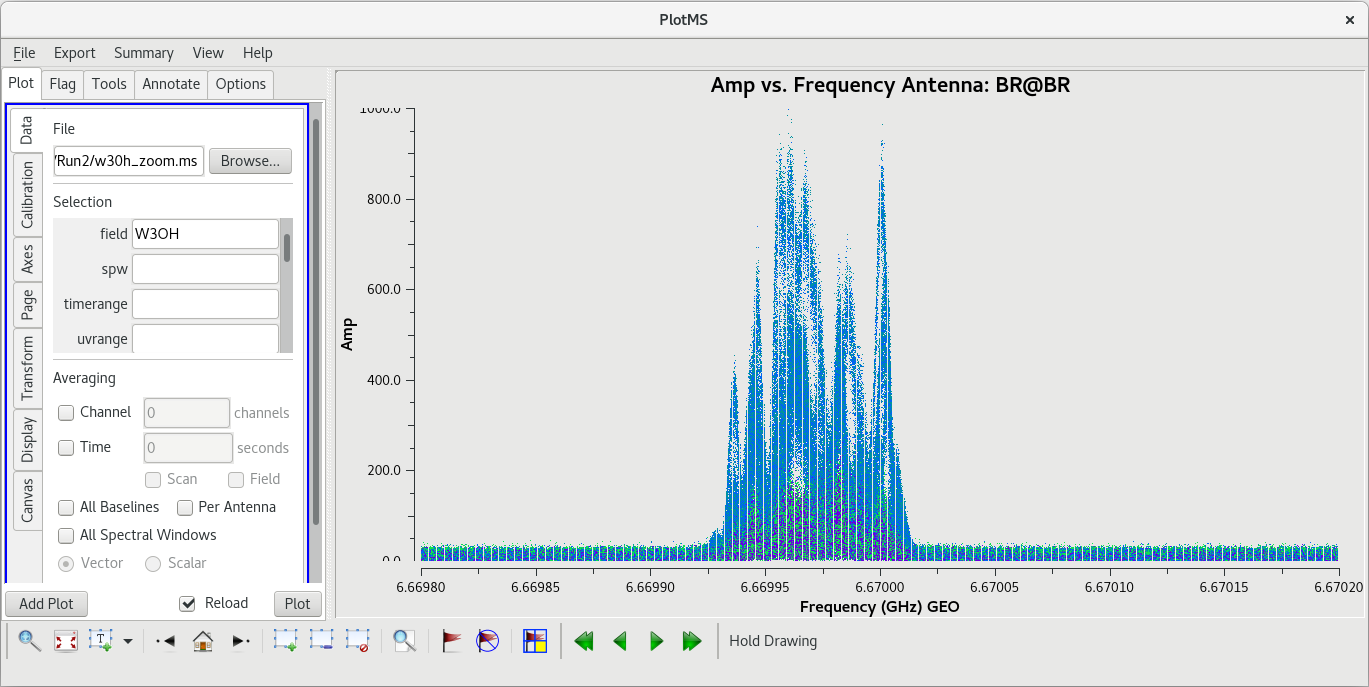
You should see a large spread in the frequencies of the maser line. This is due to different regions of W3OH having different velocities, and therefore different Doppler shifts. To properly image the maser lines, we will need to know both the location in the field and the frequency of the lines at that location.
Now, we will finally make images of the masers. There are a few differences between making these images and when we made continuum images of the phase reference calibrator. Namely, we will use specmode='cube'.
There are actually many masers in our field of view. To make one image with all of them, you will need a large amount of memory (RAM). This should only be attempted on an NRAO cluster node, or a computer with at least 32 GB of RAM (preferably 64 GB). Also, be warned that it may take you all day to make one image. For those who are interested in trying to make this large image cube, here are the reocmmended tclean inputs: vis='w3oh_zoom.ms', field='W3OH', spw='0:240~440', imsize=[1620], cell=['0.2mas'], stokes='I', specmode='cube', restfreq='6668.5192MHz', deconvolver='hogbom', weighting='natural', niter=100000, interactive=True, savemodel='none'. Good luck.
For this tutorial, we will cheat a little and make two small image cubes of select maser regions rather than one huge image cube.
A NOTE ON BEST PRACTICES: When making VLBA image cubes of targets like masers, it is best to create separate clean masks for each spectral channel (this is part of the reason that making the big image of the entire field might take all day; you need to create several unique masks for each spectral channel). Because the maser line has a Doppler shift, it will not be equally bright in each spectral channel and its position is different in each spectral channel. If you define a single clean mask for all specrtral channels, you could clean noise and/or artifacts in the channels without maser emission. However, if the area of interest is small enough that the restoring beam sidelobes are not going to contaminate other parts of the image, you can get away with only defining one clean mask for all spectral channels.
We will start with something relatively easy. There is a region in the southern part of our target region with a single bright maser confined to a relatively small number of spectral channels. The region is also small enough that we should be able to avoid problems with the sidelobes, so we can define a single clean mask for all of the spectral channels. We will use tclean in the interactive mode and set specmode='cube'. We will also need to shift the center of the image to the location of the maser using the phasecenter parameter. Finally, we need to provide the rest frequency of the maser line, which is 6668.5192MHz.
#In CASA
tclean(vis='w3oh_zoom.ms', field='W3OH', spw='0:276~304', imagename='W3OH_zoom_South', imsize=[200], cell=['0.2mas'], phasecenter='J2000 02:27:03.823 +61.52.25.084', stokes='I', specmode='cube', restfreq='6668.5192MHz', deconvolver='hogbom', weighting='natural', niter=10000, interactive=True, savemodel='none')
The interactive clean GUI will open showing the first spectral channel in our selected range. You should not see anything in there, yet. In the right-hand panel under "Channels", click on the Play button to step through all of the channels we have selected for this cube. You should see the maser line become very obvious in fourth or fifth spectral channel. It will appear to move from right to left as the display steps through the spectral channels. Notice that some artifacts start to become obvious in the tenth or eleventh spectral channel. These are the sidelobes in our beam. Fortunately, the maser in this region is confined to a region small enough that the sidelobes will not overlap any of the maser emission. So, we can be lazy and just define a single clean mask for all of the spectral channels. Click the Stop button once you have watched the display step through all of the channels a few times.
In the green region in the upper left, select "All Channels". Any time we add a clean mask in one spectral channel, it will apply to all spetral channels. Use the Forward Step button (right-pointing triangle with vertical line on right-hand side) to step through the spectral channels until you get to one where the maser emission is obvious. Use you favorite mask drawing tool (I tend to use the Ellipse tool for this one) to draw the first clean mask. Step through more channels and add mask components that cover all of the maser emission in every spectral channel. Once you have a mask defined and you are confident it covers all of the obvious maser emission, click the "Continue deconvolution" button (circular green arrow in upper right of the green region) to start the clean process.
 |
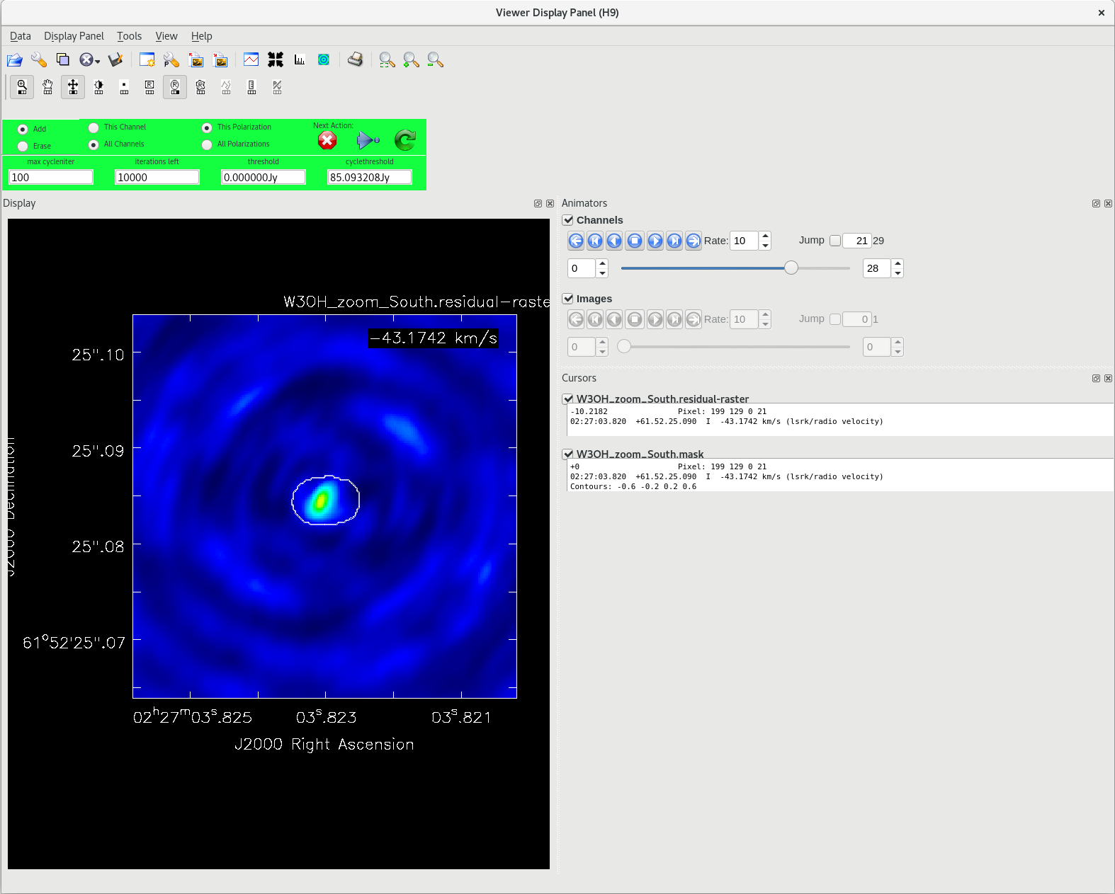 |
When the first round of cleaning finishes, you will get a new set of residual images. Step through them and enlarge your clean mask to get all of the maser emission you can see now that the noise is reduced. Once your larger clean mask is set, click the "Continue deconvolution" button again to continue cleaning. Go through this process until the maser region is noise-like in all spectral channels. When you are done cleaning, click the "Stop deconvolving now" button (red cirlce with the white 'X' in the middle). Several new files will be created in you directory, including the image file "W3OH_zoom_South.image".
You can inspect the image cube with the CASA viewer or with CARTA. For this tutorial, we will use the viewer
#In CASA
imview
This will open a new window. Click on the File icon (just below "Data" in the top row) and look for your image cube file. Select the image cube file and click "raster image". This will display a colorscale version of the image cube. Click the Play button to step through all of the spectral windows. You should see the maser get brighter and move from right to left in the display.
Now that we have an image cube, let's do a little spectral analysis. We'll make a position-velocity diagram. In order to do this, we will need to describe a "slit" (a straight line in pixel space) along the maser's path as we step through the spectral channels. Our maser appears to move almost perfectly horizontally, so the y pixel position should not change much. Looking at the lower spectral channels, we will start our "slit" at x=126, y=102 (just to the west/right of the maser in the lower spectral channels). Stepping through the spectral channels, we will end our slit at x=79, y=102. Use the CASA task impv to create the position-velocity diagram.
#In CASA
impv(imagename='W3OH_zoom_South.image', outfile='W3OH_zoom_South_PV1.image', mode='coords', start=[126,102], end=[79,102])
This will make a new file called "W3OH_zoom_South_PV1.image", which you can open with the CASA viewer.
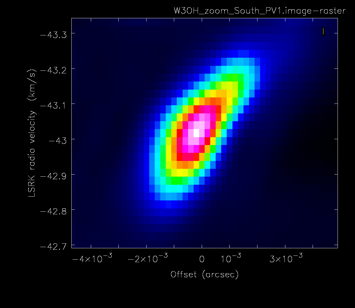 |
Now that we have done an easy example of imaging a maser region, let's try something more challenging. We will make an image cube of a region near the center of our pointing. This region has several masers, and they are separated in both space and frequency. Because there are multiple masers in the area and the region is larger than for our first image, we will need to make separate clean masks for each spectral channel.
#In CASA
tclean(vis='w3oh_zoom.ms', field='W3OH', spw='0:300~342', imagename='W3OH_zoom_Center', imsize=[320], cell=['0.2mas'], phasecenter='J2000 02:27:03.818 +61.52.25.209', stokes='I', specmode='cube', restfreq='6668.5192MHz', deconvolver='hogbom', weighting='natural', niter=10000, interactive=True, savemodel='none')
Make sure that you have "This Channel" selected (in the green region) so that you create clean masks for each spectral channel separately. When stepping through the spectral channels for the dirty image, it may not be obvious what is a maser and what is an sidelobe artifact. To start with, only mask the brightest objects in a spectral channel. After cleaning a little, it will become more obvious what is a real maser. You will need to update the clean masks each time you get a new residual image. Keep an eye on the Remaining Iterations box in the interactive clean window. You will likely see the number get pretty low before you decide to stop cleaning. If you run out of iterations, you can start tclean again and pick up where you left off as long as restart=True (which is the default) and all of the image parameters (imagename, imsize, cell, etc.) are the same as the previous execution.
Once you are done cleaning and have created your image cube of the central region, take a look at it with the CASA viewer.
#In CASA
imview
Open the file "W3OH_zoom_Center.image" as a raster image. Click the Play button to step through the spectral channels. You should see a complicated region with several masers appearing, moving, and disappearing.
Congratulations! You have calibrated and imaged a VLBA spectral line observation in CASA!
