CARMA spectral line mosaic M99 3.1: Difference between revisions
| (31 intermediate revisions by 3 users not shown) | |||
| Line 4: | Line 4: | ||
== Overview == | == Overview == | ||
[[Image:m99a.jpg|thumb|KPNO optical composite image of M99 in the Virgo Cluster (NOAO/AURA/NSF). North is approximately pointing to the right in this image.]] | |||
This tutorial describes the data reduction for CO (1-0) data observed toward the galaxy M99 (NGC 4254) using CARMA. | This tutorial describes the data reduction for CO (1-0) data observed toward the galaxy M99 (NGC 4254) using CARMA. | ||
These data were kindly provided by the CARMA STING team and should not be used for scientific purposes. More information about STING and these data in particular can be found in Rahman et al. (2010) and [http://www.astro.umd.edu/~bolatto/STING/ CARMA STING webpage]. | These data were kindly provided by the CARMA STING team and should not be used for scientific purposes. More information about STING and these data in particular can be found in Rahman et al. (2010) and [http://www.astro.umd.edu/~bolatto/STING/ CARMA STING webpage]. | ||
CO (1-0) observations are a standard method used by millimeter astronomers to estimate the distribution of molecular gas in galaxies. Most of this gas is actually molecular hydrogen (H2), but without a dipole moment H2 is not able to emit effectively under the physical conditions where it is found (T < 50 K, n > 100 cm^-3). CO is the next most common molecule (though less abundant by a factor of 10^-4) and its low rotational transitions are easily excited in most molecular clouds. As a result, the CO lines are (for now) the bread-and-butter for extragalactic millimeter science. | |||
In this tutorial we follow common CARMA practice to utilize a wide band (500 MHz) spectral window to calibrate narrow band ( | |||
Observations like these can be used in a number of ways. Rahman et al. (2010) compared these data to maps of Halpha, infrared, and UV emission to | |||
study the link between molecular gas and star formation in M99. By compiling observations of multiple CO transitions or combining with | |||
observations of other molecules, these data can be used to study how the physical conditions inside the molecular gas vary across the galaxy (e.g., see Wilson et al. 2009 for a multi-transition study of M99). The velocity of the gas, traced by the doppler shift of the CO line, can be used to measure the total mass of the galaxy (including dark matter), infer the orientation of the disk, estimate Coriolis forces and shear in the gas, and search for deviations from the simple case of a rotating disk. | |||
In this tutorial we follow common CARMA practice to utilize a wide band (500 MHz) spectral window to calibrate narrow band (60 MHz) spectral windows in order to achieve better signal-to-noise. | |||
==Getting the Data== | |||
The tutorial below assumes that you have followed the initial MIRIAD data reduction and export to fits steps described at | The tutorial below assumes that you have EITHER followed the initial MIRIAD data reduction and export to fits steps described at | ||
[[Extracting data from MIRIAD]] | [[Extracting data from MIRIAD]], OR if you want to skip the miriad steps, you can download the resulting fits files from | ||
http://casa.nrao.edu/Data/CARMA/M99/M99_CARMA.fits.tar | |||
After downloading, unpack the data in the directory you will be working in with | After downloading, unpack the data in the directory you will be working in with | ||
| Line 19: | Line 28: | ||
tar -xvf M99_CARMA.fits.tar | tar -xvf M99_CARMA.fits.tar | ||
this will create a directory called fits. | this will create a directory called fits. The tutorial assumes that you are working one level above the fits directory. | ||
== How to Use This casaguide== | |||
[[Image:clean.png|thumb|Example of inputs for the clean task.]] | |||
There are a number of possible ways to run CASA. Many aspects are described in [[Getting_Started_in_CASA]]. You should review this page if you are new to CASA. In brief you can run CASA interactively by looking at the inputs to tasks with '''inp taskname''' (example: inp clean), setting the parameters one by one (example: selectdata=T) as you desire and then run '''go'''. After setting parameters one by one in a task and then looking at the inputs again, you will notice that the parameters that have been set to something other than their defaults are blue. If you have mistyped any parameters, they will be red and must be fixed for the task to run correctly. You can get more detailed help on any task by typing '''help taskname''' (example: help clean). Once a task is run you can get the same parameters back by running '''tget taskname''' (example: tget clean); subsequent runs will overwrite the previous tget file. | |||
The second way to run CASA is to provide task function calls. This tutorial is made up of such calls, which were developed by looking at the inputs for each task and deciding what needed to be changed from default values. For task function calls, '''only parameters that you want to be different from their defaults need to be set'''. A series of task function calls can be combined together into a script, and run with '''execfile('scriptname.py')'''. It is possible to extract a script containing all the CASA task function calls in this and other casaguides using the method described at the [[Extracting_scripts_from_these_tutorials]] page. | |||
If you are a relative novice or just new to CASA it is strongly recommended to work through this tutorial by cutting and pasting the task function calls provided below after you have read all the associated explanations, and work at your own pace, look at the inputs to the tasks to see what other options exist, and read the help files. Later when you are more comfortable, you might try extracting the script, modify it for your purposes and begin to reduce other data. | |||
== Import fits files == | == Import fits files == | ||
| Line 29: | Line 47: | ||
for i in range(4,7): | for i in range(4,7): | ||
msfile = "c0104I"+str(i)+".ms" | msfile = "c0104I"+str(i)+".ms" | ||
importuvfits(fitsfile="fits/c0104I."+str(i)+".fits", | importuvfits(fitsfile="fits/c0104I."+str(i)+".fits",vis=msfile) | ||
myfiles.append(msfile) | myfiles.append(msfile) | ||
</source> | </source> | ||
| Line 64: | Line 81: | ||
tb.close() | tb.close() | ||
</source> | </source> | ||
Now look at the listobs output again. | |||
<source lang="python"> | <source lang="python"> | ||
| Line 446: | Line 465: | ||
</source> | </source> | ||
== Calibrate Absolute Flux == | == Calibrate the Absolute Flux Scale== | ||
<source lang="python"> | <source lang="python"> | ||
| Line 481: | Line 500: | ||
</source> | </source> | ||
Notice spwmap=[[0,0,0],[0,0,0],[0,0,0]]. For this call, spwmap was not strictly necessary because the default spwmap=[] | '''Notice spwmap=[[0,0,0],[0,0,0],[0,0,0]]'''. For this call, spwmap was not strictly necessary because the default spwmap=[] | ||
would have had the same effect. This default means for each calibration table specified in gaintable, apply the corresponding solutions from the specified spw(s) to itself. There are as many [] entries in spwmap as there are tables specified in gaintable, and there are as many spw entries per [] list as the total number of spw in the data. For example, if there had been 6 spw in this dataset, and 4 (instead of 3) tables to apply one would write spwmap=[[0,0,0,0,0,0],[0,0,0,0,0,0],[0,0,0,0,0,0],[0,0,0,0,0,0]]. | would have had the same effect. This default means for each calibration table specified in gaintable, apply the corresponding solutions from the specified spw(s) to itself. There are as many [] entries in spwmap as there are tables specified in gaintable, and there are as many spw entries per [] list as the total number of spw in the data. For example, if there had been 6 spw in this dataset, and 4 (instead of 3) tables to apply one would write spwmap=[[0,0,0,0,0,0],[0,0,0,0,0,0],[0,0,0,0,0,0],[0,0,0,0,0,0]]. | ||
They need to be specified in the same order as the table order in gaintable, though the order in gaintable itself is arbitrary. | They need to be specified in the same order as the table order in gaintable, though the order in gaintable itself is arbitrary. | ||
Now for spw='1,2', we see the real power of spwmap | '''Notice gainfield=['1','1','1']'''. This parameter lets us specify which source the solutions should come from. Again, there should be as many entries as calibration tables specified in gaintable, and the gainfield entries need to be in the same order as gaintable, though the order in gaintable itself is arbitrary. | ||
spw 0 is not specified in the spw parameter, we must still have | |||
Now for the narrowband data (spw='1,2'), we see the real power of spwmap. This parameter is what allows us to tell {{applycal}} to use the wideband spw phase and amplitude solutions (0), but the narrowband bandpass solutions as appropriate for each spw independently. Note that even though spw 0 is not specified in the spw parameter, we must still have placeholders for it in each spwmap parameter (i.e. the first 0 in the latter two lists). | |||
<source lang="python"> | <source lang="python"> | ||
| Line 513: | Line 533: | ||
[[Image:M99plotmsfina.png|thumb|Amplitudes after calibration.]] | [[Image:M99plotmsfina.png|thumb|Amplitudes after calibration.]] | ||
For the target we will use both gain calibrators, | For the target, we will use both gain calibrators ('1,21') for phase calibration in {{applycal}}, because both are close in position on the sky to the target. Whichever is closest in time will be applied to the target. We will also use both for flux calibration. However, it is important to note that for more typical millimeter observations, the flux calibrator (usually a planet or minor planet) is often *not* close to the target on the sky and should not be used for phase calibration. In this case, the field entry in the gainfield list corresponding to the flux calibration table will differ from the entry corresponding to the phase calibration table. | ||
<source lang="python"> | <source lang="python"> | ||
| Line 563: | Line 583: | ||
[[Image:M99_interactive.png|thumb|The interactive viewer with the .flux contours in magenta and the clean mask in white contours.]] | [[Image:M99_interactive.png|thumb|The interactive viewer with the .flux contours in magenta and the clean mask in white contours.]] | ||
The clean call below, uses the interactive clean mode. This is important for complex extended emission as is seen in the CO(1-0) for M99. Below we provide a brief description of one easy way you might make a clean mask for this image. Of course making a clean mask for each channel individually would be better if you have the time and patience. | The clean call below, uses the interactive clean mode. This is important for complex extended emission as is seen in the CO(1-0) for M99. Below we provide a brief description of one easy way you might make a clean mask for this image. Of course making a clean mask for each channel individually would be better if you have the time and patience. | ||
'''Note''' The {{clean}} task automatically knows that if imagermode='mosaic' and it sees that there are multiple antenna dish sizes in the data, that it should use the heterogenous array mode for calculating the primary beam response. If you are doing a single field CARMA reduction you still want to chose imagermode='mosaic' so that the primary beam response will be properly calculated for the heterogenous array case. | |||
<source lang="python"> | <source lang="python"> | ||
| Line 579: | Line 601: | ||
When the interactive viewer pops up (this may take a few minutes), click the "folder" icon in top left. From file GUI select "M99_cube_nearest.flux" and then click "Contour Map" under "Display As". This will show the convolution of the primary beam coverage. Next click the "wrench" next to the file folder icon. This will open the "Data Display Options" GUI. At the top, tab over until you see the "M99_cube_nearest.flux-contour" tab. | When the interactive viewer pops up (this may take a few minutes), click the "folder" icon in top left. From file GUI select "M99_cube_nearest.flux" and then click "Contour Map" under "Display As". This will show the convolution of the primary beam coverage. Next click the "wrench" next to the file folder icon. This will open the "Data Display Options" GUI. At the top, tab over until you see the "M99_cube_nearest.flux-contour" tab. | ||
Now change the line color to magenta (from foreground). Now click the zoom button in the Display panel and zoom in on the mosaic region. Chose "all channels" toggle in the green box and then chose the "Polygon drawing" tool from the top, and make a clean mask around the outermost contour (this happens to be the 0.2 contour level). Double click inside the polygon area (with the same button you used to define the polygon), and you should see it turn | Now change the line color to magenta (from foreground). Now click the zoom button in the Display panel and zoom in on the mosaic region. Chose "all channels" toggle in the green box and then chose the "Polygon drawing" tool from the top, and make a clean mask around the outermost contour (this happens to be the 0.2 contour level). Double click inside the polygon area (with the same button you used to define the polygon), and you should see it turn magenta. If you now use the frame slider commands below the image to move back and forth through the cube, you can check that all the emission falls within the masked region. | ||
Once you are satisfied with the mask, '''go to the data drop down menu and close the "M99_cube_nearest.flux-contour" file. If you don't do this you will get a table lock and the final image will not be constructed.''' Then hit the blue arrow to continue cleaning with this mask until the threshold is reached. More clean masking tips and techniques are described in the [[EVLA spectral line IRC10216]] casaguide. | Once you are satisfied with the mask, '''go to the data drop down menu and close the "M99_cube_nearest.flux-contour" file. If you don't do this you will get a table lock and the final image will not be constructed.''' Then hit the blue arrow to continue cleaning with this mask until the threshold is reached. More clean masking tips and techniques are described in the [[EVLA spectral line IRC10216]] casaguide. | ||
| Line 591: | Line 613: | ||
</source> | </source> | ||
Then use the | Then use the frame slider to go to a line free channel, select the box region tool and make a box. When you double click in the box, the image statistics for the channel you are on will print to the terminal. Move the box around a bit to see what the variation is. You should get something like 20 - 25 mJy (it will be on the high end of this range in channels with line emission). If you want the box tool to go away, hit the escape key. | ||
Next make integrated intensity maps (moment 0) and integrated velocity maps (moment 1). | Next make integrated intensity maps (moment 0) and integrated velocity maps (moment 1). To do this, we'll want to know what channels the line emission starts and ends on. The first channel with significant emission is channel 1, while the last channel with significant emission is channel 23. | ||
[[Image:moment_maps_2.png|thumb|Example of moment 0 and moment 1 images side by side.]] | [[Image:moment_maps_2.png|thumb|Example of moment 0 and moment 1 images side by side.]] | ||
| Line 602: | Line 624: | ||
axis='spectral', | axis='spectral', | ||
chans='1~23',outfile='M99_cube.moment0') | chans='1~23',outfile='M99_cube.moment0') | ||
</source> | </source> | ||
| Line 620: | Line 643: | ||
</source> | </source> | ||
You can open both moment maps as rasters and then blink between them by first clicking the "blink" toggle and then using the | You can open both moment maps as rasters and then blink between them by first clicking the "blink" toggle and then using the frame slider to cycle through. You might also try opening the "p wrench tool" (Viewer Canvas Manager) at the top of the Viewer display panel, then go to "Number of panels" and up the number in x to 2. Then if its not already selected, click blink in the Viewer display to see both images side by side. It will help to make your viewer window fairly wide. | ||
Also try opening the moment1 as a raster and moment0 as a contour map (In the example at right, I've played with the default contour levels in the "Data display options"). | Also try opening the moment1 as a raster and moment0 as a contour map (In the example at right, I've played with the default contour levels in the "Data display options"). | ||
During the imaging process, the primary beam response of the different antennas was taken into account to form the mosaic and properly weight the different contributions, but we have not yet '''corrected''' the images for the response. In this sense the images are not yet, ''flux correct'' -- instead, the mosaic appears to have constant noise, instead of the reality where the rms noise increases towards the edges of the mosaiced region. The primary beam response (taking into account the mosaic and the heterogeneous nature of CARMA) is saved in the ''imagename.flux'' image. Have a look at it now with the viewer. | |||
<source lang="python"> | |||
viewer(infile='M99_cube_nearest.flux') | |||
</source> | |||
Then use the folder icon to open the file browser and select M99_cube_nearest.image. Then use the '''blink''' toggle to blink between them. Notice that near the center of the mosaic the .flux image is one and that this gets smaller and smaller towards the edges. To correct for this primary beam response, you divide the .image by the .flux. | |||
<source lang="python"> | |||
immath(imagename=['M99_cube_nearest.image','M99_cube_nearest.flux'], | |||
expr='IM0/IM1',outfile='M99_cube_nearest.pbcor') | |||
</source> | |||
Now load this new image into the viewer you already have open (or reopen it if you closed it) to check the effect. For analysis that involves the true flux density like the moment 0, column density etc, you should use this primary beam corrected map. However, now the noise is considerably higher near the edges (as it should be). Try remaking the moment 0 image with the corrected cube (M99_cube_nearest.pbcor). | |||
For publication, you may wish to denote the half-power point of the mosaic by overlaying a dashed contour on the moment zero map. This can be done in the viewer. First load the moment map as a raster image. Then load the .flux image as a contour map. Then click the wrench tool and select the second tab (i.e. the flux image tab). Change the relative contour levels to [0.5], then select "Dash positive contours?" to "True". | |||
{{Checked 3.0.2}} | {{Checked 3.0.2}} | ||
--[[User:CBrogan|Crystal Brogan]] | --[[User:CBrogan|Crystal Brogan]] | ||
{{Checked 3.1.0}} | |||
Latest revision as of 21:27, 26 May 2011
Overview
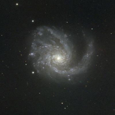
This tutorial describes the data reduction for CO (1-0) data observed toward the galaxy M99 (NGC 4254) using CARMA. These data were kindly provided by the CARMA STING team and should not be used for scientific purposes. More information about STING and these data in particular can be found in Rahman et al. (2010) and CARMA STING webpage. CO (1-0) observations are a standard method used by millimeter astronomers to estimate the distribution of molecular gas in galaxies. Most of this gas is actually molecular hydrogen (H2), but without a dipole moment H2 is not able to emit effectively under the physical conditions where it is found (T < 50 K, n > 100 cm^-3). CO is the next most common molecule (though less abundant by a factor of 10^-4) and its low rotational transitions are easily excited in most molecular clouds. As a result, the CO lines are (for now) the bread-and-butter for extragalactic millimeter science.
Observations like these can be used in a number of ways. Rahman et al. (2010) compared these data to maps of Halpha, infrared, and UV emission to study the link between molecular gas and star formation in M99. By compiling observations of multiple CO transitions or combining with observations of other molecules, these data can be used to study how the physical conditions inside the molecular gas vary across the galaxy (e.g., see Wilson et al. 2009 for a multi-transition study of M99). The velocity of the gas, traced by the doppler shift of the CO line, can be used to measure the total mass of the galaxy (including dark matter), infer the orientation of the disk, estimate Coriolis forces and shear in the gas, and search for deviations from the simple case of a rotating disk.
In this tutorial we follow common CARMA practice to utilize a wide band (500 MHz) spectral window to calibrate narrow band (60 MHz) spectral windows in order to achieve better signal-to-noise.
Getting the Data
The tutorial below assumes that you have EITHER followed the initial MIRIAD data reduction and export to fits steps described at Extracting data from MIRIAD, OR if you want to skip the miriad steps, you can download the resulting fits files from
http://casa.nrao.edu/Data/CARMA/M99/M99_CARMA.fits.tar
After downloading, unpack the data in the directory you will be working in with
tar -xvf M99_CARMA.fits.tar
this will create a directory called fits. The tutorial assumes that you are working one level above the fits directory.
How to Use This casaguide
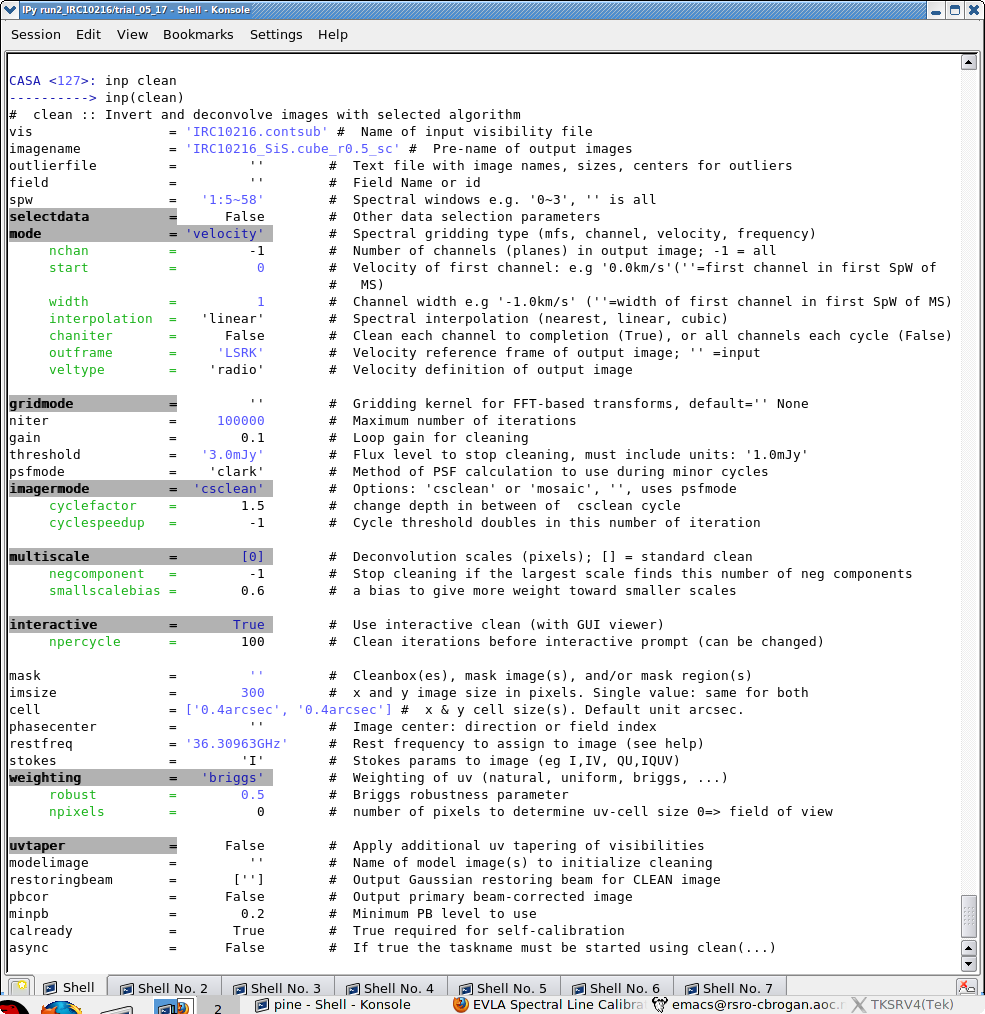
There are a number of possible ways to run CASA. Many aspects are described in Getting_Started_in_CASA. You should review this page if you are new to CASA. In brief you can run CASA interactively by looking at the inputs to tasks with inp taskname (example: inp clean), setting the parameters one by one (example: selectdata=T) as you desire and then run go. After setting parameters one by one in a task and then looking at the inputs again, you will notice that the parameters that have been set to something other than their defaults are blue. If you have mistyped any parameters, they will be red and must be fixed for the task to run correctly. You can get more detailed help on any task by typing help taskname (example: help clean). Once a task is run you can get the same parameters back by running tget taskname (example: tget clean); subsequent runs will overwrite the previous tget file.
The second way to run CASA is to provide task function calls. This tutorial is made up of such calls, which were developed by looking at the inputs for each task and deciding what needed to be changed from default values. For task function calls, only parameters that you want to be different from their defaults need to be set. A series of task function calls can be combined together into a script, and run with execfile('scriptname.py'). It is possible to extract a script containing all the CASA task function calls in this and other casaguides using the method described at the Extracting_scripts_from_these_tutorials page.
If you are a relative novice or just new to CASA it is strongly recommended to work through this tutorial by cutting and pasting the task function calls provided below after you have read all the associated explanations, and work at your own pace, look at the inputs to the tasks to see what other options exist, and read the help files. Later when you are more comfortable, you might try extracting the script, modify it for your purposes and begin to reduce other data.
Import fits files
Below we show an example of creating a python dictionary and using "for" loops in python to run importuvfits multiple times, and then use the output as the input to the concat task.
myfiles = []
for i in range(4,7):
        msfile = "c0104I"+str(i)+".ms"
        importuvfits(fitsfile="fits/c0104I."+str(i)+".fits",vis=msfile)
        myfiles.append(msfile)
concat(vis=myfiles,concatvis='c0104I',timesort=True)
listobs(vis='c0104I')
Look at the logger output. Notice that the CARMA data comes into CASA with antenna names that are numbers and that CASA also creates an antenna ID number for each antenna (it also creates ID numbers for fields and spw). Both the antenna name and ID can be used to identify an antenna, which is very confusing if both are numbers -- but not the same number. The python commands below will append the antenna names with CA to more easily distinguish them from their IDs. ALMA will already have antenna names that are strings, as does the EVLA. This step is only needed for data that comes into CASA via importuvfits.
tb.open("c0104I/ANTENNA",nomodify=False)
namelist=tb.getcol("NAME").tolist()
for i in range(len(namelist)):
	name = 'CA'+namelist[i]
	print ' Changing '+namelist[i]+' to '+name
	namelist[i]=name

tb.putcol("NAME",namelist)
tb.close()
Now look at the listobs output again.
listobs(vis='c0104I')
 Fields: 22
   ID   Code Name         RA            Decl           Epoch   nVis
   0         MARS         09:15:50.0585 +17.21.03.8918 J2000   9450
   1         3C273        12:29:06.7000 +02.03.08.5980 J2000   60480
   2         NGC4254      12:18:47.8090 +14.24.13.9342 J2000   24570
   3         NGC4254      12:18:49.6000 +14.24.13.9342 J2000   24570
   4         NGC4254      12:18:51.3910 +14.24.13.9342 J2000   24570
   5         NGC4254      12:18:52.2865 +14.24.36.4672 J2000   24570
   6         NGC4254      12:18:50.4955 +14.24.36.4672 J2000   24570
   7         NGC4254      12:18:48.7045 +14.24.36.4672 J2000   24570
   8         NGC4254      12:18:46.9135 +14.24.36.4672 J2000   24570
   9         NGC4254      12:18:46.0179 +14.24.59.0000 J2000   24570
   10        NGC4254      12:18:47.8090 +14.24.59.0000 J2000   24570
   11        NGC4254      12:18:49.6000 +14.24.59.0000 J2000   24570
   12        NGC4254      12:18:51.3910 +14.24.59.0000 J2000   24570
   13        NGC4254      12:18:53.1821 +14.24.59.0000 J2000   24570
   14        NGC4254      12:18:52.2865 +14.25.21.5328 J2000   24570
   15        NGC4254      12:18:50.4955 +14.25.21.5328 J2000   24570
   16        NGC4254      12:18:48.7045 +14.25.21.5328 J2000   24570
   17        NGC4254      12:18:46.9135 +14.25.21.5328 J2000   22680
   18        NGC4254      12:18:47.8090 +14.25.44.0658 J2000   22680
   19        NGC4254      12:18:49.6000 +14.25.44.0658 J2000   22680
   20        NGC4254      12:18:51.3910 +14.25.44.0658 J2000   22680
   21        3C274        12:30:49.4230 +12.23.28.0440 J2000   45360
    (nVis = Total number of time/baseline visibilities per field)
 Spectral Windows:  (3 unique spectral windows and 1 unique polarization setups)
   SpwID  Chans Frame Ch1(MHz)    ChanWid(kHz)TotBW(kHz)  Ref(MHz)    Corrs
   0          15 LSRK  113978.067  31250       468750      113978.067  RR
   1          63 LSRK  114289.671  976.5625    61523.4375  114289.671  RR
   2          63 LSRK  114341.036  976.5625    61523.4375  114341.036  RR
 The SOURCE table is empty: see the FIELD table
 Antennas: 15:
   ID   Name  Station   Diam.    Long.         Lat.
   0    CA1     ANT1      10.4 m   -116.45.01.0  +37.13.43.4
   1    CA2     ANT2      10.4 m   -116.59.48.3  +37.52.00.3
   2    CA3     ANT3      10.4 m   -120.06.43.6  +37.35.02.8
   3    CA4     ANT4      10.4 m   -119.38.33.8  +38.26.22.2
   4    CA5     ANT5      10.4 m   -119.13.25.0  +35.03.23.4
   5    CA6     ANT6      10.4 m   -119.06.39.2  +38.54.24.4
   6    CA7     ANT7      6.1  m   -119.30.34.9  +36.58.55.6
   7    CA8     ANT8      6.1  m   -118.08.34.0  +37.16.45.8
   8    CA9     ANT9      6.1  m   -118.46.59.9  +36.48.41.4
   9    CA10    ANT10     6.1  m   -118.29.04.6  +36.03.45.6
   10   CA11    ANT11     6.1  m   -118.48.40.9  +37.15.57.8
   11   CA12    ANT12     6.1  m   -119.33.27.5  +36.06.46.1
   12   CA13    ANT13     6.1  m   -118.31.43.5  +37.05.19.4
   13   CA14    ANT14     6.1  m   -118.13.18.7  +36.50.34.6
   14   CA15    ANT15     6.1  m   -117.23.50.2  +36.25.48.2
Since you were (likely) not the original observer for these data, here is a basic overview of how we will use them:
Observing Strategy:

Bandpass, Gain, and Flux calibrator: 3c273 field ID=1
Secondary Gain Calibrator 3C274 field ID=21
Extra flux calibrator Mars field ID=0

The target mosaic (M99) is in field IDs 2~20

There is one wideband channel (spw=0) and two narrow band channels
(spw=1,2)
Initial Inspection and Flagging
First, flag edge channels:
flagdata(vis='c0104I',mode='manualflag',selectdata=True,spw='0:0~1;13~14')
flagdata(vis='c0104I',mode='manualflag',selectdata=True,spw='1~2:0~1;61~62')
Let's look at the wide band channel on all sources:
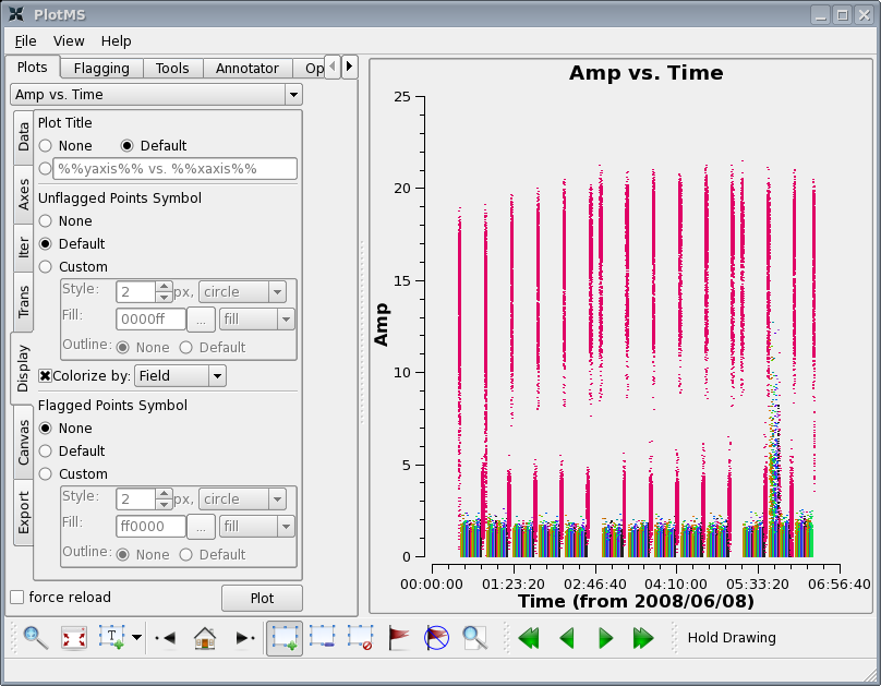
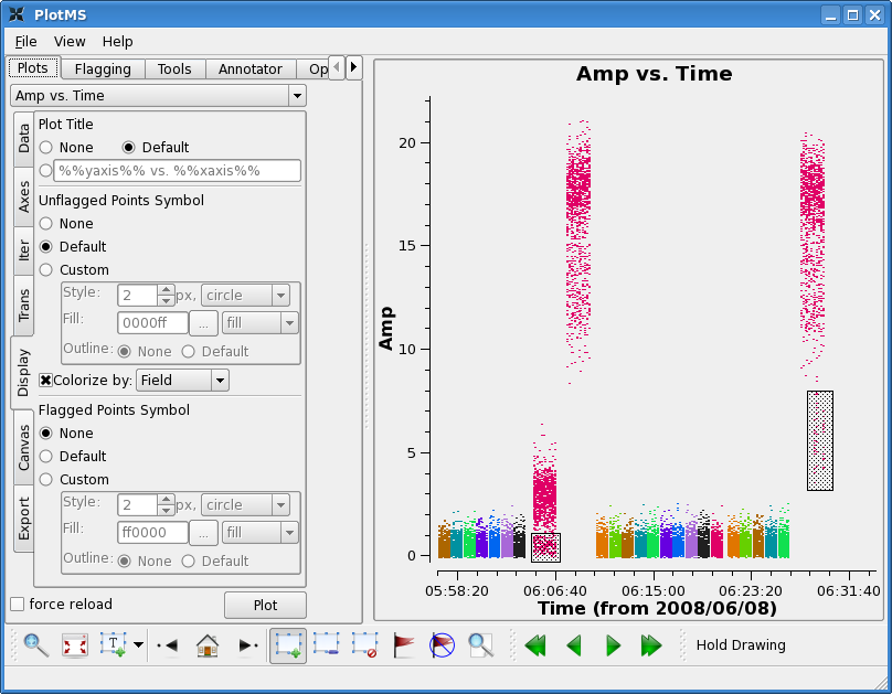
plotms(vis='c0104I',xaxis='time',yaxis='amp',field='1~21', spw='0',
      avgchannel='15')
Click "Display" tab in the plotms GUI and select "Colorize by: Field", then click the plot button.
There are a few things to notice:
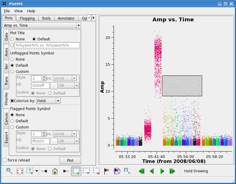
First there is some very noticeably bad target data near the end of the observation. Use the zoom button to zoom in on the bad timerange, click the Mark Region icon and put a box over a modest number of the offending high points, and then press the Locate button.
Information about the located points will display to the terminal (not the Log Messages window). This will tell you that the offending telescope is antenna name=CA13 (id=12) and that the field-ids are 2~11. Looking at the plot the bad time range is 05:43:00~05:54:00.
Click the "Clear Regions" button, and then the "house" button to
unzoom.
Next note that the first two scans on 3c273 and the last scan on
3c273 show some low points. Also the last scan on 3c274 shows low
points. Again use zoom, mark, and locate to see if you can see a
pattern.
The first two scans on 3c273 don't show a particular pattern -- no particular antenna or individual time range appears to be responsible. This is usually a good indication that it cannot be calibrated out. Also note that it is unlikely that the target data in between is good, though this is not obvious because the target is weak. However, 3c274 does look ok, before the second 3c273 scan. Unfortunately, there is no way to calibrate the first target scans even if they are good, with no calibrator scan to precede them. For now we will flag 3c273 scans and the target in that timerange.
As for the last scans, there is a pattern: problems with the last scan on 3c273 appears to be caused by antenna CA7 (in scan 272) and problems with the last scan on 3c274 appears to be related to antenna CA8 (scan 255).
Looking at the lowest points on all the 3c273 scans, baseline CA2-CA8 appears low, we will also wait to see if this calibrates out.
We will flag the narrow band channels wherever we see problems in wideband. You can either make separate plotting commands, or combine as below. To demonstrate different possibilities we use timerange to identify some data, and scan number to identify others.
flagdata(vis='c0104I',spw='0~2',
	 antenna=['CA13','','CA7','CA8'],
	 field=['2~11','1~20','1','21'],
	 scan=['','','272','255'],
	 timerange=['05:43:00~05:54:00','00:25:00~00:55:00','',''])
Note that each of these flagging commands could have been written out separately, but combining them into one command will run much faster than the combined time of multiple calls as the data only have to be searched once.
Set the Absolute Flux Scale
Often for millimeter observations, the absolute flux scale is determined by observing a planet and using a model of its flux as a function of baseline length (most planets are not point sources at mm frequencies using typical arrays). This is because the flux of planets change in a mostly predictable way (depending primarily on distance at any given time) than quasars. CASA does not yet have this functionality (we expect it for the next release). The flux of 3c273 is inserted from CARMA flux monitoring (which used the Mars observation to derive the 3c273 flux). Note that the first argument to the fluxdensity parameter is the Stokes I (total intensity).
setjy(vis='c0104I', field='3C273',fluxdensity=[17.8,0.,0.,0.], spw='0~2')
Transferring Gains from One Spectral Window to Another
Below we lay out in detail the steps for using the wideband gain calibration for the narrowband CARMA data. There are a few important things to note about this procedure:
(1) There are two essential calibrations that must be done: Bandpass as a function of frequency (amplitude and phase) and Gain as a function of time (amplitude and phase).
(2) Each spectral window (spw) will have independent bandpass shapes in both amplitude and phase.
(3) As long as the system is relatively stable with time, the gain calibrations are typically the same for each spectral window after the full bandpass dependence is removed.
In a dataset where each spw calibrates only itself, one typically normalizes the bandpass solutions, so that they take out the shape of the bandpass (in amplitude and phase), but not the absolute amplitude or phase offsets (which vary from spw to spw). In that case the gain solutions contain both the phase and amplitude solutions as a function of time, but also the absolute bandpass amplitude and phase offsets. The CASAguide EVLA spectral line IRC10216 provides an example of this procedure.
By contrast, in a case where you want to apply the gain calibrations from one spw to another, you definitely do not want those gains to apply the absolute bandpass amplitude and phase offsets derived from one spw to another. This is why in the steps below, we use solnorm=F in the bandpass task. This forces the absolute bandpass amplitude and phase offsets to be contained in the bandpass solutions (which are derived independently for each spw).
Calibrate the Wideband Bandpass
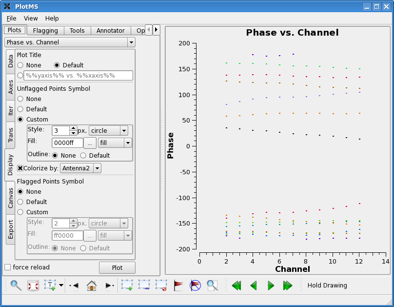
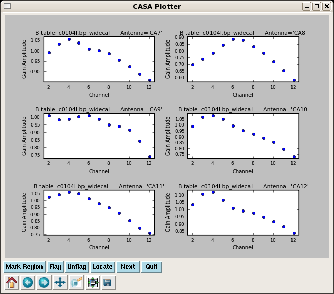
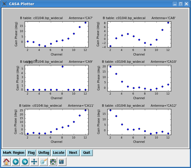
Lets start by looking at the bandpass calibrator's phase as a function of channel for the wideband data.
plotms(vis='c0104I',xaxis='channel',yaxis='phase',
       field='1',spw='0',antenna='CA1',
       avgtime='1e8',avgscan=T)
Select colorize by antenna2, and select "custom" for unflagged points, and then raise the style to 3 to make the plotted points easier to see. You will see that the phase does not change a great deal on individual baselines over the wide band channel (spw=0). This means that averaging over some channels will not introduce significant closure errors. Check other antennas if you like.
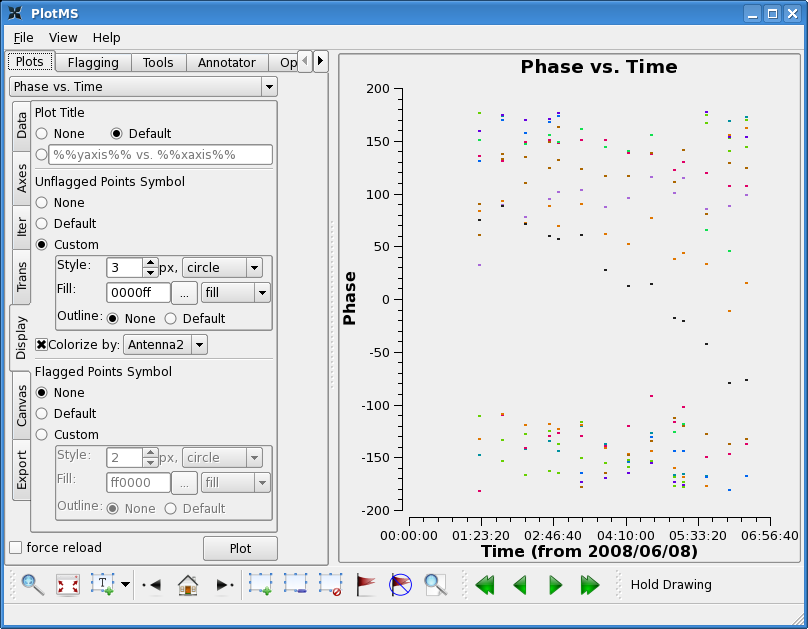
Now look at the phase as a function of time. With avgtime a large number, but no avgscan=T, this command will show the average phase per scan. Since the cache changes, the colorize option changes too. You will have to select these again as above.
plotms(vis='c0104I',xaxis='time',yaxis='phase',
       field='1',spw='0',
       antenna='CA1',
       avgchannel='15',avgtime='1e8')
Here you see significant variation with time. This is not surprising as the bandpass calibrator was observed over a fairly long period of time (~6 hours). In this case, it is important to calibrate the phase before solving for the bandpass. We choose a fairly narrow channel range since the bandpass phase as a function of frequency has not been taken out yet (though for these data it is quite well behaved).
gaincal(vis='c0104I',caltable='c0104I.bpphase_widecal',
        field='1',spw='0:5~9',
        refant='CA9',calmode='p',solint='inf',minsnr=2.0)
The use of solint='inf' here without setting combine will get one solution per scan.
Look at the solutions:
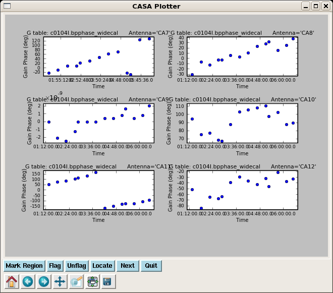
plotcal(caltable='c0104I.bpphase_widecal',
        xaxis='time',yaxis='phase',
        iteration='antenna',subplot=321)
Note the phase drift is > 100 degrees on some antennas -- this is why it would not have been appropriate to vector average these data into one bp solution before taking out the phase. Use the "Next" button to page through all antennas.
Having done a preliminary phase solution we can now combine all the 3C273 scans into one bandpass solution. Note the default combine parameter is different for bandpass : combine='scan'.
bandpass(vis='c0104I',caltable='c0104I.bp_widecal',
         interp='',field='1',spw='0',
         bandtype='B',solint='inf',
         refant='CA9',solnorm=F,
         gaintable=['c0104I.bpphase_widecal'],
         spwmap=[[]])
Note that you will see warning messages "Insufficient unflagged antennas to proceed with this solve" for the channels that were flagged previously. This behavior is expected and does not indicate a problem. Next, plot the amplitude and phase of the wideband bandpass solutions.
plotcal(caltable='c0104I.bp_widecal',xaxis='chan',yaxis='amp',
        iteration='antenna',subplot=321)
plotcal(caltable='c0104I.bp_widecal',xaxis='chan',yaxis='phase',
        iteration='antenna',subplot=321)
Calibrate the Wideband Gains
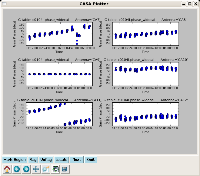
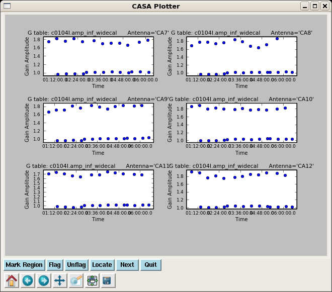
Now resolve for phase and also amplitude while applying the bandpass solutions, for both calibrators 3c273 and 3c274. We will not use the first gain solution again.
First, do a phase solution on the timescale of an individual integration. (Consulting the listobs will reveal that each scan is about 5 minutes long, built up of 10-second integrations.)
gaincal(vis='c0104I',caltable='c0104I.phase_widecal',
        field='1,21',spw='0',
        refant='CA9',calmode='p',solint='int',minsnr=2.0,
        gaintable=['c0104I.bp_widecal'],
        spwmap=[[]])
plotcal(caltable='c0104I.phase_widecal',xaxis='time',yaxis='phase',
        iteration='antenna',subplot=321,plotrange=[0,0,-180,180])
Note the significant phase variation within a single scan. If we used an average phase over each whole scan to derive the amplitude solutions, it would decorrelate the subsequent amplitude corrections.
So use the phase calibration just derived to get an amplitude solution over each scan:
gaincal(vis='c0104I',caltable='c0104I.amp_inf_widecal',
        field='1,21',spw='0',
        refant='CA9',calmode='ap',solint='inf',minsnr=2.0,
        gaintable=['c0104I.bp_widecal','c0104I.phase_widecal'],
        spwmap=[[]])
plotcal(caltable='c0104I.amp_inf_widecal',xaxis='time',yaxis='amp',
        iteration='antenna',subplot=321)
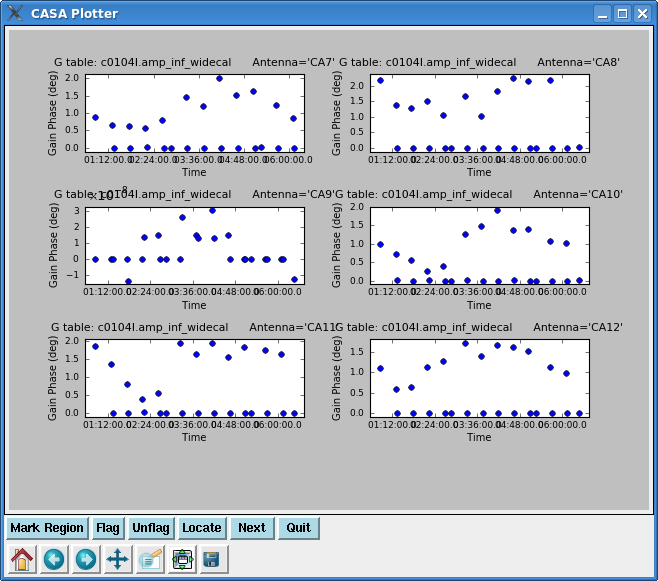
Note the different gains for 3c273 scans and 3c274 scans, this just reflects that the two calibrators have different strengths.
Next plot the phase from the amplitude solutions -- this will be the residual phase after taking out the integration-time based solutions. This gives a good idea of the residual phase noise. If this is more than a few degrees, the cause should be investigated. Note that the scatter for 3c274 is larger than 3c273 -- this reflects that 3c274 is significantly weaker and thus has lower S/N.
plotcal(caltable='c0104I.amp_inf_widecal',xaxis='time',yaxis='phase',
        iteration='antenna',subplot=321)
Here we re-run the phase only calibration but now getting one solution per scan to apply later to the target. An alternative would be to smooth the integration time phase calibration table, but this is a bit simpler.
gaincal(vis='c0104I',caltable='c0104I.phase_inf_widecal',
        field='1,21',spw='0',
        refant='CA9',calmode='p',solint='inf',minsnr=2.0,
        gaintable=['c0104I.bp_widecal'],
        spwmap=[[]])
plotcal(caltable='c0104I.phase_inf_widecal',xaxis='time',yaxis='phase',
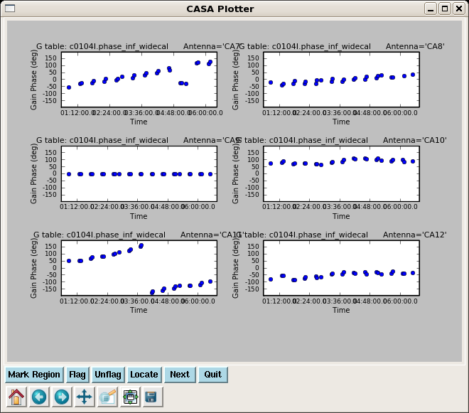
        iteration='antenna',subplot=321,plotrange=[0,0,-180,180])
This is a very important plot to look at carefully as these are the phase solutions that will be applied to the target. Note that the phases for 3c273 and 3c274 are very similar, but not exactly the same. Unfortunately we can not color by field here to make it easier to see.
Calibrate the Narrow Band Bandpasses
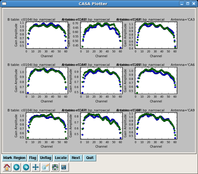
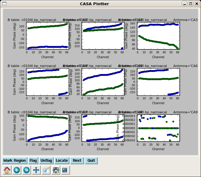
Solve for the narrow band bandpasses, applying the time-dependent phase and amplitude corrections derived from the wideband data. Because there are 3 spw in the data, you must set a placeholder for all three in spwmap, even though we are only solving for 2 of them.
bandpass(vis='c0104I',caltable='c0104I.bp_narrowcal',
         interp='',field='1',spw='1,2',
         bandtype='B',solint='inf',
         refant='CA9',solnorm=F,
         gaintable=['c0104I.phase_widecal','c0104I.amp_inf_widecal'],
         spwmap=[[0,0,0],[0,0,0]])
plotcal(caltable='c0104I.bp_narrowcal',xaxis='chan',yaxis='amp',
        iteration='antenna',subplot=331)
plotcal(caltable='c0104I.bp_narrowcal',xaxis='chan',yaxis='phase',
        iteration='antenna',subplot=331)
Calibrate the Absolute Flux Scale
fluxscale(vis='c0104I',caltable='c0104I.amp_inf_widecal',
          fluxtable='c0104I.fluxcal',reference='1')
The derived flux density for the other calibrator will be printed in the logger. It is a good idea to copy these lines for future reference.
Flux density for 3C274 in SpW=0 is: 3.11626 +/- 0.0146614
     (SNR = 212.549, nAnt= 15)
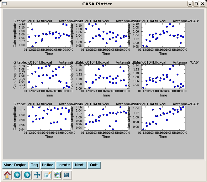
Check that the flux table looks reasonable; as the raw fluxes of the calibrators were close to their measured values in Jy, it is not surprising that the points for each antenna are clustered around 1.0.
plotcal(caltable='c0104I.fluxcal',xaxis='time',yaxis='amp',
        iteration='antenna',subplot=331)
Applycal and Inspect
We run applycal separately for the wide and narrow band data so we can apply the appropriate bandpass tables.
Applying solutions to 3C273, first for the wideband data (spw='0'):
applycal(vis='c0104I',field='1',spw='0',
        gaintable=['c0104I.bp_widecal','c0104I.phase_widecal',
        'c0104I.fluxcal'],
        spwmap=[[0,0,0],[0,0,0],[0,0,0]],gainfield=['1','1','1'])
Notice spwmap=[[0,0,0],[0,0,0],[0,0,0]]. For this call, spwmap was not strictly necessary because the default spwmap=[] would have had the same effect. This default means for each calibration table specified in gaintable, apply the corresponding solutions from the specified spw(s) to itself. There are as many [] entries in spwmap as there are tables specified in gaintable, and there are as many spw entries per [] list as the total number of spw in the data. For example, if there had been 6 spw in this dataset, and 4 (instead of 3) tables to apply one would write spwmap=[[0,0,0,0,0,0],[0,0,0,0,0,0],[0,0,0,0,0,0],[0,0,0,0,0,0]]. They need to be specified in the same order as the table order in gaintable, though the order in gaintable itself is arbitrary.
Notice gainfield=['1','1','1']. This parameter lets us specify which source the solutions should come from. Again, there should be as many entries as calibration tables specified in gaintable, and the gainfield entries need to be in the same order as gaintable, though the order in gaintable itself is arbitrary.
Now for the narrowband data (spw='1,2'), we see the real power of spwmap. This parameter is what allows us to tell applycal to use the wideband spw phase and amplitude solutions (0), but the narrowband bandpass solutions as appropriate for each spw independently. Note that even though spw 0 is not specified in the spw parameter, we must still have placeholders for it in each spwmap parameter (i.e. the first 0 in the latter two lists).
applycal(vis='c0104I',field='1',spw='1,2',
        gaintable=['c0104I.bp_narrowcal','c0104I.phase_widecal',
        'c0104I.fluxcal'],
        spwmap=[[],[0,0,0],[0,0,0]],gainfield=['1','1','1'])
Applying solutions to 3C274:
applycal(vis='c0104I',field='21',spw='0',
        gaintable=['c0104I.bp_widecal','c0104I.phase_widecal',
        'c0104I.fluxcal'],
        spwmap=[],gainfield=['1','21','21'])
applycal(vis='c0104I',field='21',spw='1,2',
        gaintable=['c0104I.bp_narrowcal','c0104I.phase_widecal',
        'c0104I.fluxcal'],
        spwmap=[[],[0,0,0],[0,0,0]],gainfield=['1','21','21'])
For the target, we will use both gain calibrators ('1,21') for phase calibration in applycal, because both are close in position on the sky to the target. Whichever is closest in time will be applied to the target. We will also use both for flux calibration. However, it is important to note that for more typical millimeter observations, the flux calibrator (usually a planet or minor planet) is often *not* close to the target on the sky and should not be used for phase calibration. In this case, the field entry in the gainfield list corresponding to the flux calibration table will differ from the entry corresponding to the phase calibration table.
applycal(vis='c0104I',field='2~20',spw='0',
        gaintable=['c0104I.bp_widecal','c0104I.phase_inf_widecal',
        'c0104I.fluxcal'],
        spwmap=[],gainfield=['1','1,21','1,21'])
applycal(vis='c0104I',field='2~20',spw='1,2',
        gaintable=['c0104I.bp_narrowcal','c0104I.phase_inf_widecal',
        'c0104I.fluxcal'],
        spwmap=[[],[0,0,0],[0,0,0]],gainfield=['1','1,21','1,21'])
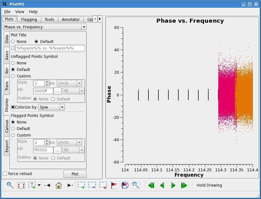
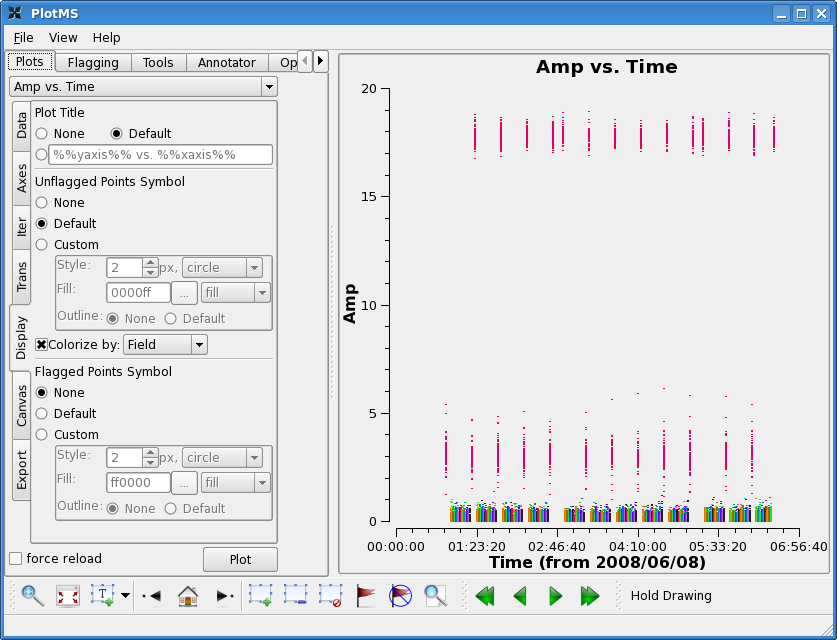
You should now see, for example, that the phases are flat across all spw for 3C273, and amplitudes match the monitored calibrator fluxes for this date (with the source data at the bottom).
plotms(vis='c0104I',xaxis='frequency',ydatacolumn='corrected',
       field='1',avgtime='1e8')
plotms(vis='c0104I',xaxis='time',yaxis='amp',ydatacolumn='corrected',
       field='1~21',spw='0',
       avgchannel='15',avgtime='1e8')
Deconvolution and Imaging
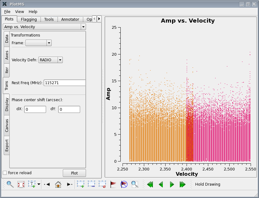
plotms(vis='c0104I',xaxis='velocity',yaxis='amp',ydatacolumn='corrected',
       field='2',spw='1~2',avgtime='1e8')
in plotms in the Trans tab set the CO rest frequency (115271.2 MHz) in order to see the velocity range of the narrow band channels (don't forget to click Plot again). Unfortunately the individual pointings are a bit too weak to see the UV vector averaged CO signal but you can at least see the observed velocity range.
Go to Display tab and choose colorize by spw. Notice that the edge channels are a bit noisy -- especially a concern in the overlap region. We will exclude these below.
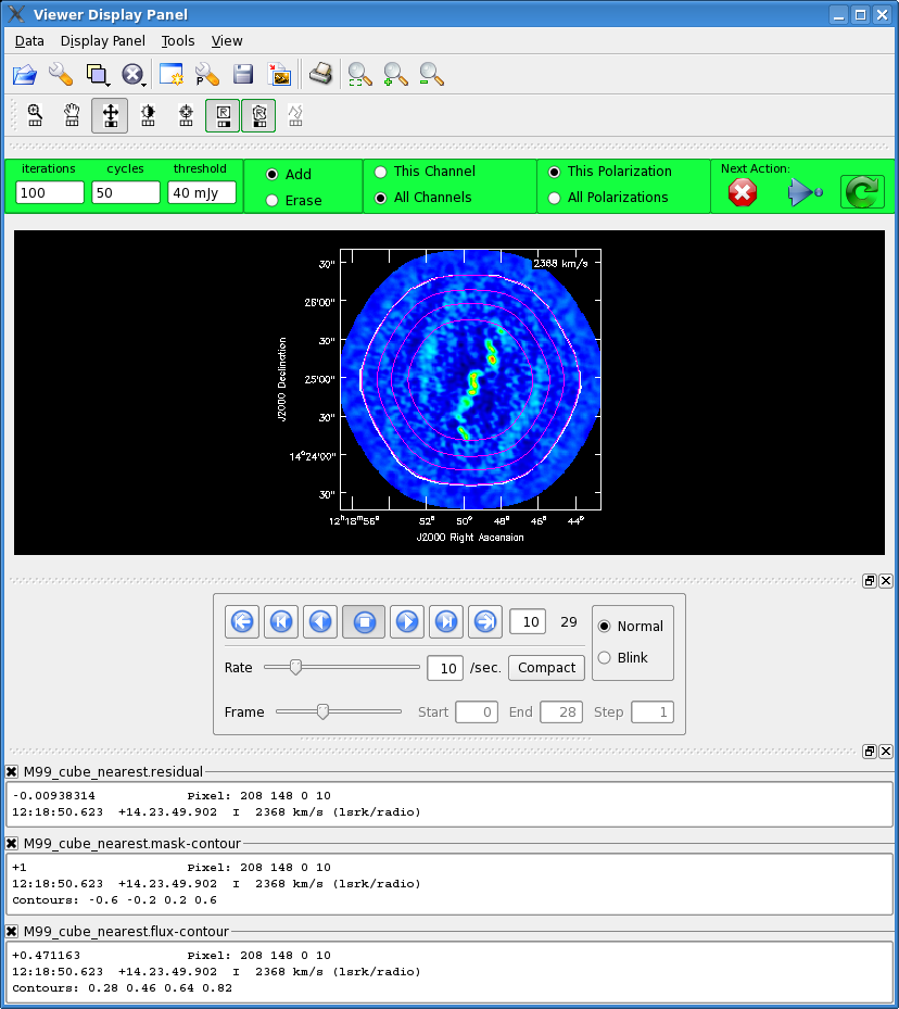
The clean call below, uses the interactive clean mode. This is important for complex extended emission as is seen in the CO(1-0) for M99. Below we provide a brief description of one easy way you might make a clean mask for this image. Of course making a clean mask for each channel individually would be better if you have the time and patience.
Note The clean task automatically knows that if imagermode='mosaic' and it sees that there are multiple antenna dish sizes in the data, that it should use the heterogenous array mode for calculating the primary beam response. If you are doing a single field CARMA reduction you still want to chose imagermode='mosaic' so that the primary beam response will be properly calculated for the heterogenous array case.
clean(vis='c0104I',imagename='M99_cube_nearest',spw='1~2:3~59',field='2~20',
      phasecenter='11',
      cell='0.9arcsec',imsize=450,
      mode='velocity',start='2268km/s',width='10.0km/s',
      interpolation='nearest',
      imagermode='mosaic',cyclefactor=2,
      restfreq='115.2712GHz',interactive=T,
      minpb=0.1,pbcor=F,
      niter=5000,threshold='40mJy')
When the interactive viewer pops up (this may take a few minutes), click the "folder" icon in top left. From file GUI select "M99_cube_nearest.flux" and then click "Contour Map" under "Display As". This will show the convolution of the primary beam coverage. Next click the "wrench" next to the file folder icon. This will open the "Data Display Options" GUI. At the top, tab over until you see the "M99_cube_nearest.flux-contour" tab.
Now change the line color to magenta (from foreground). Now click the zoom button in the Display panel and zoom in on the mosaic region. Chose "all channels" toggle in the green box and then chose the "Polygon drawing" tool from the top, and make a clean mask around the outermost contour (this happens to be the 0.2 contour level). Double click inside the polygon area (with the same button you used to define the polygon), and you should see it turn magenta. If you now use the frame slider commands below the image to move back and forth through the cube, you can check that all the emission falls within the masked region.
Once you are satisfied with the mask, go to the data drop down menu and close the "M99_cube_nearest.flux-contour" file. If you don't do this you will get a table lock and the final image will not be constructed. Then hit the blue arrow to continue cleaning with this mask until the threshold is reached. More clean masking tips and techniques are described in the EVLA spectral line IRC10216 casaguide.
Image Analysis
First lets see what the rms noise level in a single channel is using the viewer.
viewer(infile='M99_cube_nearest.image')
Then use the frame slider to go to a line free channel, select the box region tool and make a box. When you double click in the box, the image statistics for the channel you are on will print to the terminal. Move the box around a bit to see what the variation is. You should get something like 20 - 25 mJy (it will be on the high end of this range in channels with line emission). If you want the box tool to go away, hit the escape key.
Next make integrated intensity maps (moment 0) and integrated velocity maps (moment 1). To do this, we'll want to know what channels the line emission starts and ends on. The first channel with significant emission is channel 1, while the last channel with significant emission is channel 23.
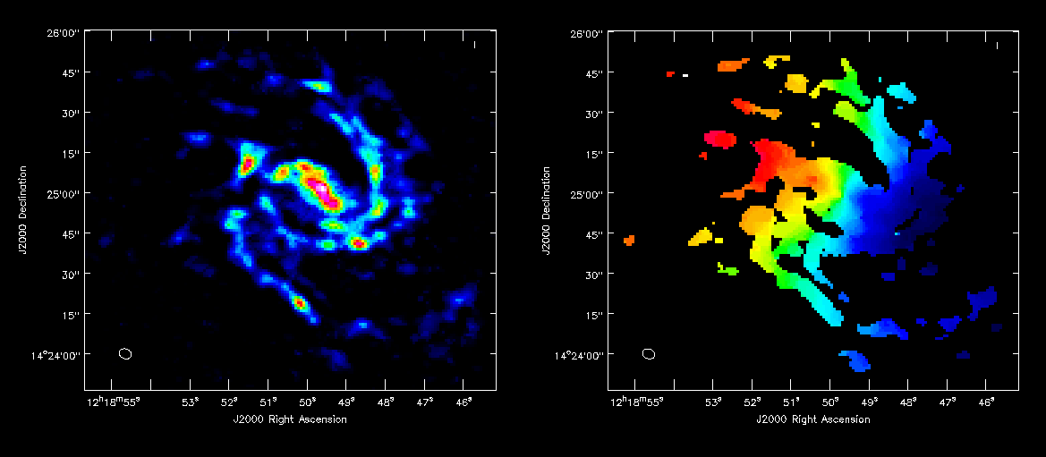
For moment zero, its best to limit the calculation to image channels with significant signal in them, but not to apply a flux cutoff, as this will bias the derived integrated intensities upward.
immoments(imagename='M99_cube_nearest.image',moments=[0],
          axis='spectral',
          chans='1~23',outfile='M99_cube.moment0')
For moment 1, it is essential to apply a conservative flux cutoff to limit the calculation to high signal-to-noise areas. Here we use about 5sigma.
immoments(imagename='M99_cube_nearest.image',moments=[1],
          axis='spectral',
          chans='1~23',excludepix=[-100,0.125],
          outfile='M99_cube.moment1')
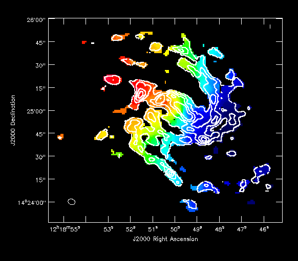
Next you can open the viewer by typing
viewer
You can open both moment maps as rasters and then blink between them by first clicking the "blink" toggle and then using the frame slider to cycle through. You might also try opening the "p wrench tool" (Viewer Canvas Manager) at the top of the Viewer display panel, then go to "Number of panels" and up the number in x to 2. Then if its not already selected, click blink in the Viewer display to see both images side by side. It will help to make your viewer window fairly wide.
Also try opening the moment1 as a raster and moment0 as a contour map (In the example at right, I've played with the default contour levels in the "Data display options").
During the imaging process, the primary beam response of the different antennas was taken into account to form the mosaic and properly weight the different contributions, but we have not yet corrected the images for the response. In this sense the images are not yet, flux correct -- instead, the mosaic appears to have constant noise, instead of the reality where the rms noise increases towards the edges of the mosaiced region. The primary beam response (taking into account the mosaic and the heterogeneous nature of CARMA) is saved in the imagename.flux image. Have a look at it now with the viewer.
viewer(infile='M99_cube_nearest.flux')
Then use the folder icon to open the file browser and select M99_cube_nearest.image. Then use the blink toggle to blink between them. Notice that near the center of the mosaic the .flux image is one and that this gets smaller and smaller towards the edges. To correct for this primary beam response, you divide the .image by the .flux.
immath(imagename=['M99_cube_nearest.image','M99_cube_nearest.flux'],
       expr='IM0/IM1',outfile='M99_cube_nearest.pbcor')
Now load this new image into the viewer you already have open (or reopen it if you closed it) to check the effect. For analysis that involves the true flux density like the moment 0, column density etc, you should use this primary beam corrected map. However, now the noise is considerably higher near the edges (as it should be). Try remaking the moment 0 image with the corrected cube (M99_cube_nearest.pbcor).
For publication, you may wish to denote the half-power point of the mosaic by overlaying a dashed contour on the moment zero map. This can be done in the viewer. First load the moment map as a raster image. Then load the .flux image as a contour map. Then click the wrench tool and select the second tab (i.e. the flux image tab). Change the relative contour levels to [0.5], then select "Dash positive contours?" to "True".
Last checked on CASA Version 3.0.2 (r11631).
Last checked on CASA Version 3.1.0.