First Look at Image Analysis CASA 6.5.4: Difference between revisions
Tag: Undo |
|
| (One intermediate revision by the same user not shown) | |
(No difference)
| |
Latest revision as of 14:15, 8 February 2024
About this Guide
Last checked on CASA Version 6.5.4
This guide features CARTA, the “Cube Analysis and Rendering Tool for Astronomy,” which is the new NRAO visualization tool for images and cubes. The CASA viewer (imview) has not been maintained for a few years and will be removed from future versions of CASA. We strongly recommend using CARTA, as it provides a much more efficient, stable, and feature rich user experience. A comparison of the CASA viewer and CARTA, as well as instructions on how to use CARTA at NRAO, is provided in the CARTA section of the CASA docs.
The first few tutorials provided us with a spectral line data cube and a continuum image. Next we'd like to understand some of the properties of the images that we have produced.
In case you don't have the images from the first tutorials handy, let's start by copying the image files from the working directory in the full data package (download instructions are at First_Look_at_Imaging_CASA_6.5.4) to our current directory:
# In CASA - comment these out if you are using the extracted script and you want to use your own images from completing the line imaging tutorial
os.system('rm -rf twhya_cont.image')
os.system('cp -r ../working/twhya_cont.image .')
os.system('rm -rf twhya_n2hp.image')
os.system('cp -r ../working/twhya_n2hp.image .')
You can also simply download them with your browser at https://bulk.cv.nrao.edu/almadata/public/ALMA_firstlooks/twhya_cont.image and https://bulk.cv.nrao.edu/almadata/public/ALMA_firstlooks/twhya_n2hp.image .
If you do have images from the prior tutorials, you'll want fifth_image.image (our best continuum image) from the self-cal tutorial, which you will substitute for twhya_cont.image in the commands here, and twhya_n2hp.image from the spectral line imaging tutorial.
Recall that we orient ourselves with measurement sets (UV data) using the listobs task. For images, an analogous way to get basic header information is to use the imhead task.
# In CASA
imhead('twhya_cont.image')
imhead('twhya_n2hp.image')
CASA prints the image header information to the logger:
imhead::::casa  ##########################################
imhead::::casa  ##### Begin Task: imhead             #####
imhead::::casa  imhead( imagename='twhya_cont.image', mode='summary', hdkey='', hdvalue='', verbose=False )
ImageMetaData::summary
ImageMetaData::summary+ Image name       : twhya_cont.image
ImageMetaData::summary+ Object name      : TW Hya
ImageMetaData::summary+ Image type       : PagedImage
ImageMetaData::summary+ Image quantity   : Intensity
ImageMetaData::summary+ Pixel mask(s)    : mask0
ImageMetaData::summary+ Region(s)        : None
ImageMetaData::summary+ Image units      : Jy/beam
ImageMetaData::summary+ Restoring Beam   : 0.609236 arcsec, 0.452453 arcsec, -51.5786 deg
ImageMetaData::summary
ImageMetaData::summary+ Direction reference : J2000
ImageMetaData::summary+ Spectral  reference : LSRK
ImageMetaData::summary+ Velocity  type      : RADIO
ImageMetaData::summary+ Rest frequency      : 3.72637e+11 Hz
ImageMetaData::summary+ Pointing center     :  11:01:51.796000  -34.42.17.366000
ImageMetaData::summary+ Telescope           : ALMA
ImageMetaData::summary+ Observer            : cqi
ImageMetaData::summary+ Date observation    : 2012/11/19/07:56:26.544000
ImageMetaData::summary+ Telescope position: [2.22514e+06m, -5.44031e+06m, -2.48103e+06m] (ITRF)
ImageMetaData::summary+
ImageMetaData::summary+ Axis Coord Type      Name             Proj Shape Tile   Coord value at pixel        Coord incr Units
ImageMetaData::summary+ ----------------------------------------------------------------------------------------------------
ImageMetaData::summary+ 0    0     Direction Right Ascension   SIN   250  250  11:01:51.796   125.00     -1.000000e-01 arcsec
ImageMetaData::summary+ 1    0     Direction Declination       SIN   250  250 -34.42.17.366   125.00      1.000000e-01 arcsec
ImageMetaData::summary+ 2    1     Stokes    Stokes                    1    1             I
ImageMetaData::summary+ 3    2     Spectral  Frequency                 1    1   3.72637e+11     0.00 2.34445114878e+08 Hz
ImageMetaData::summary+                      Velocity                                     0     0.00     -1.886149e+02 km/s
imhead::::casa  Task imhead complete. Start time: 2023-10-06 14:07:35.341678 End time: 2023-10-06 14:07:38.267440
imhead::::casa  ##### End Task: imhead               #####
imhead::::casa  ##########################################

imhead::::casa  ##########################################
imhead::::casa  ##### Begin Task: imhead             #####
imhead::::casa  imhead( imagename='twhya_n2hp.image', mode='summary', hdkey='', hdvalue='', verbose=False )
ImageMetaData::summary
ImageMetaData::summary+ Image name       : twhya_n2hp.image
ImageMetaData::summary+ Object name      : TW Hya
ImageMetaData::summary+ Image type       : PagedImage
ImageMetaData::summary+ Image quantity   : Intensity
ImageMetaData::summary+ Pixel mask(s)    : mask0
ImageMetaData::summary+ Region(s)        : None
ImageMetaData::summary+ Image units      : Jy/beam
ImageMetaData::summary+ Restoring Beam   : 0.614894 arcsec, 0.453196 arcsec, -52.3802 deg
ImageMetaData::summary
ImageMetaData::summary+ Direction reference : J2000
ImageMetaData::summary+ Spectral  reference : LSRK
ImageMetaData::summary+ Velocity  type      : RADIO
ImageMetaData::summary+ Rest frequency      : 3.72672e+11 Hz
ImageMetaData::summary+ Pointing center     :  11:01:51.796000  -34.42.17.366000
ImageMetaData::summary+ Telescope           : ALMA
ImageMetaData::summary+ Observer            : cqi
ImageMetaData::summary+ Date observation    : 2012/11/19/07:56:26.544000
ImageMetaData::summary+ Telescope position: [2.22514e+06m, -5.44031e+06m, -2.48103e+06m] (ITRF)
ImageMetaData::summary+
ImageMetaData::summary+ Axis Coord Type      Name             Proj Shape Tile   Coord value at pixel      Coord incr Units
ImageMetaData::summary+ --------------------------------------------------------------------------------------------------
ImageMetaData::summary+ 0    0     Direction Right Ascension   SIN   250  125  11:01:51.796   125.00   -1.000000e-01 arcsec
ImageMetaData::summary+ 1    0     Direction Declination       SIN   250   50 -34.42.17.366   125.00    1.000000e-01 arcsec
ImageMetaData::summary+ 2    1     Stokes    Stokes                    1    1             I
ImageMetaData::summary+ 3    2     Spectral  Frequency                15    5  3.726725e+11     0.00 -6.21550810e+05 Hz
ImageMetaData::summary+                      Velocity                                     0     0.00    5.000000e-01 km/s
imhead::::casa  Task imhead complete. Start time: 2023-10-06 14:07:38.461741 End time: 2023-10-06 14:07:38.501495
imhead::::casa  ##### End Task: imhead               #####
imhead::::casa  ##########################################
Statistics
Often we'd like to measure basic image statistics and fluxes. Recall you can do these operations pretty easily in CARTA. You can also get statistics using the imstat task.
# In CASA
my_stats = imstat('twhya_n2hp.image', chans='0~4')
The imstat task returns a python dictionary. The imstat results are printed to the logger window, and you can examine the contents of the python dictionary as follows:
# In CASA
print(my_stats)
print(my_stats['rms'])
It's useful to see that the RMS is about 29 mJy/beam in the line cube.
You can also just print the dictionary to the terminal screen:
# In CASA
imstat('twhya_n2hp.image', chans='0~4')
This task is useful for measuring basic source characteristics. For example, calculate the statistics for a box encompassing the disk - you see that the integrated flux is about 2.0 Jy.
# In CASA
imstat('twhya_cont.image', box='100,100,150,150')
my_stats = imstat('twhya_cont.image', box='100,100,150,150')
print(my_stats['flux'])
Alternatively, a box defined off the disk will give image noise statistics.
# In CASA
imstat('twhya_cont.image', box='25,150,225,200')
This gives an RMS of 1.9 mJy, varying slightly from what we saw in the selfcal tutorial (2.0 mJy) because the region used to calculate it is different. If you want your stats to be consistent, you can draw a region in CARTA, export the region as, say, "my_region_file", and then give imstat "region = 'my_region_file'" instead of defining a simple rectangle with the "box" parameter. Just be careful not to use both parameters at once!
Moments
For the spectral line cube, it's very useful to "collapse" the cube in various ways to analyze the emission. The immoments task lets you do this.
The first few "moments" are defined as follows:
 moments = -1 : mean value of the spectral coordinate
 moments =  0 : integrated value of the spectral coordinate
 moments =  1 : intensity weighted coordinate; traditionally used to get 'velocity fields'
 moments =  2 : intensity weighted dispersion of the coordinate; traditionally used to get "velocity dispersion"
A more complete description of image moments is given in the task documentation immoments.

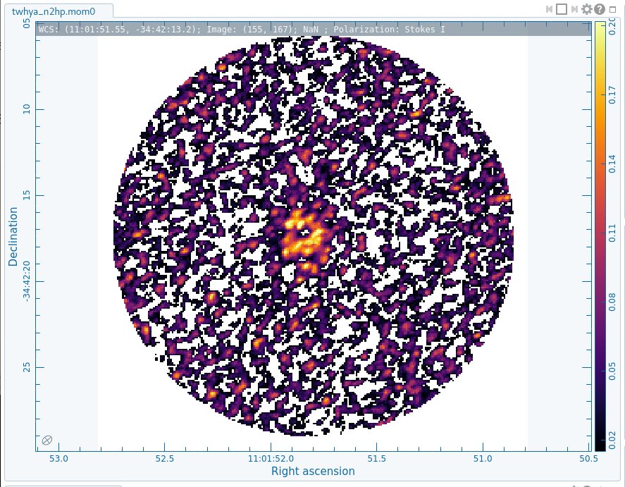
Let's make a moment 0 image, clipped at ~1 sigma (~30 mJy) to limit the amount of noise that gets included. We further restrict the channels to include the known line channels 5-7, with a buffer on either side.
# In CASA
os.system('rm -rf twhya_n2hp.mom0')
immoments('twhya_n2hp.image',
          outfile='twhya_n2hp.mom0',
          includepix=[30e-3,100],
          chans='4~12',
          moments=0)
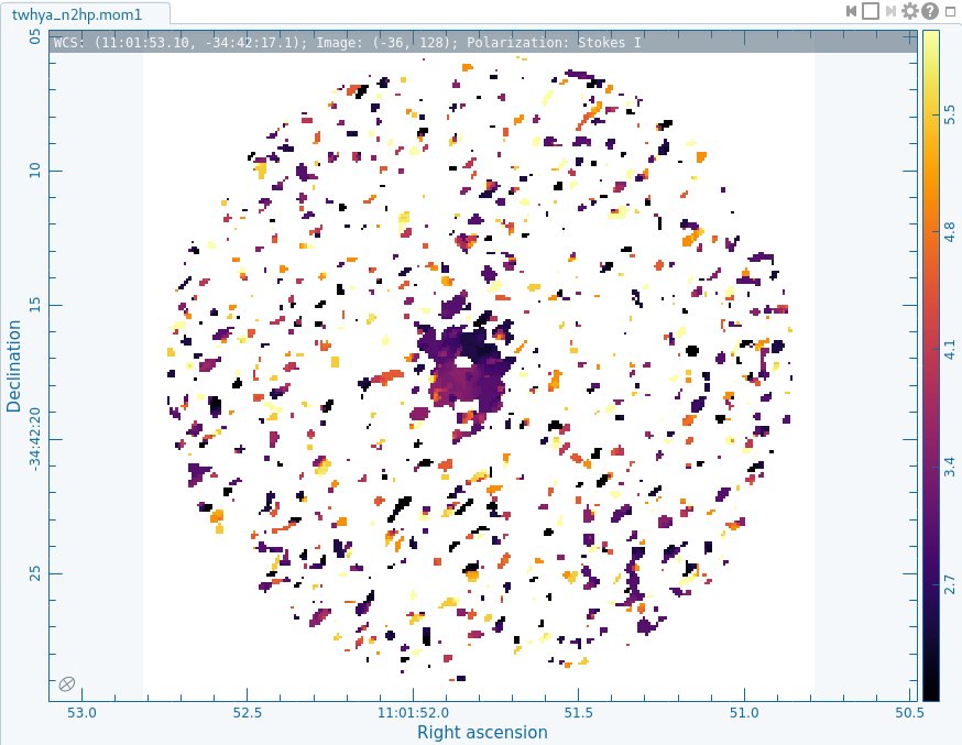
Make a moment 1 image clipped instead at ~2 sigma (~60 mJy):
# In CASA
os.system('rm -rf twhya_n2hp.mom1')
immoments('twhya_n2hp.image',
          outfile='twhya_n2hp.mom1',
          includepix=[60e-3,100],
          chans='4~12',
          moments=1)
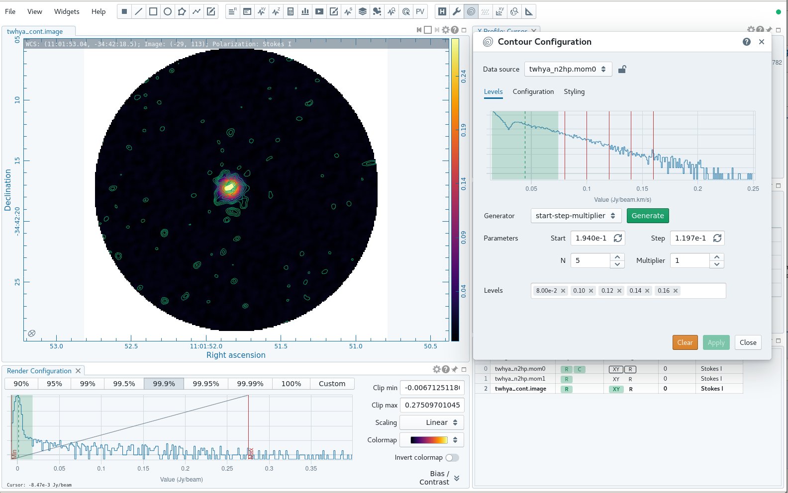
At this point we have a few really neat things to see: first the line shows a hole in the middle. Overlay it on the dust (continuum) disk using CARTA (Figure 2) and you can notice that they align but with the N2H+ existing only outside a certain radius - in this case the "snow line". Also have a look at the velocity field to see the rotation of the disk (Figure 3).
To open CARTA, if you are using NRAO machines, you can navigate to your working directory in a terminal, and then type:
# In bash
carta --no_browser
Copy the URL it returns and paste into a browser window to view your CARTA session. To overlay the N2H+ moment 0 contour in CARTA, open twhya_cont.image and twhya_n2hp.mom0 holding ctrl while clicking to select both, or open one and then use "append" to open the second file. Use the animator tab to make the continuum image the "active" image. On the "View" menu, select "Contours". Make sure the lock next to the "Data source" drop-down menu is UNlocked, so that you can choose twhya_n2hp.mom0 as the data source. You can either use the generator in this Contour Configuration pane to create the levels, or type them into the "levels" box directly. Figure 2 shows twhya_n2hp.mom0 contours at levels, in Jy, of 0.08, 0.10, 0.12, 0.14, and 0.16. You can also choose the smoothing algorithm and factor on the Configuration tab in the Contour Configuration pane, and you can choose the thickness, color, etc of the contours in the Styling tab.


Here, we are not using the primary beam corrected images and cubes when creating our moment maps. Remember that it's often very convenient to work in images before primary beam correction because the noise is the same across the field (e.g., this is a clean data set to search for signal) but it's very important to remember to apply this correction before calculating fluxes or intensities for science.
Export FITS images
CASA is great (of course) but you will ultimately want to export your data to a common format to analyze in other programs, share with other astronomers, or archive. It's easy to export images from CASA's image format to FITS images via the exportfits command.
# In CASA
exportfits(imagename='twhya_cont.image',
           fitsimage='twhya_cont.fits',
           overwrite=True)
For the cube we want to specify additionally that the frequency axis will be written out as velocity.
# In CASA
exportfits(imagename='twhya_n2hp.image',
           fitsimage='twhya_n2hp.fits',
           velocity=True,
           overwrite=True)