First Look at Line Imaging CASA 6.5.4: Difference between revisions
Tag: Manual revert |
|||
| (4 intermediate revisions by the same user not shown) | |||
| Line 10: | Line 10: | ||
provided. | provided. | ||
If you have not completed the previous tutorial, you'll need the self-calibrated data. You can download the full package for these First Look tutorials following the instructions at [[First_Look_at_Imaging_CASA_6.5.4]] Guide for instructions. The full package contains twhya_selfcal.ms.tar, or you can download twhya_selfcal.ms.tar separately at https://bulk.cv.nrao.edu/almadata/ | If you have not completed the previous tutorial, you'll need the self-calibrated data. You can download the full package for these First Look tutorials following the instructions at [[First_Look_at_Imaging_CASA_6.5.4]] Guide for instructions. The full package contains twhya_selfcal.ms.tar, or you can download twhya_selfcal.ms.tar separately at https://bulk.cv.nrao.edu/almadata/public/ALMA_firstlooks/twhya_selfcal.ms.tar . | ||
Note that it often makes good sense to self-calibrate on the continuum source, even when the main science goal is to image spectral line emission. This is especially true when the continuum is bright and not overly complex. Sometimes, though, it can make better sense to self-calibrate on a spectral line, and apply those solutions to the entire data set. For now, we will apply the continuum self-cal solutions to our spectral line data to optimize our spectral line images. | Note that it often makes good sense to self-calibrate on the continuum source, even when the main science goal is to image spectral line emission. This is especially true when the continuum is bright and not overly complex. Sometimes, though, it can make better sense to self-calibrate on a spectral line, and apply those solutions to the entire data set. For now, we will apply the continuum self-cal solutions to our spectral line data to optimize our spectral line images. | ||
| Line 42: | Line 41: | ||
plot the amplitude as a function of channel number, averaging the data over | plot the amplitude as a function of channel number, averaging the data over | ||
time. (The parameter avgscan=True tells CASA to allow time averaging across scans.) | time. (The parameter avgscan=True tells CASA to allow time averaging across scans.) | ||
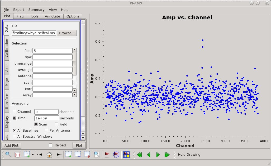
[[File:Imaging-tutorial-line-plotms-1_6.5.4.jpg|thumb|<caption>Figure 1: In this plot of amplitude vs. channel number, we can see several high amplitudes that represent detected spectral line emission. Note that the amplitudes away from the spectral line are well above zero, showing the continuum emission.</caption>]] | [[File:Imaging-tutorial-line-plotms-1_6.5.4.jpg|thumb|<caption>Figure 1: In this plot of amplitude vs. channel number, we can see several high amplitudes that represent detected spectral line emission. Note that the amplitudes away from the spectral line are well above zero, showing the continuum emission.</caption>]] | ||
<source lang="python"> | <source lang="python"> | ||
| Line 90: | Line 87: | ||
similar to what we did before, and look at the spectrum, which | similar to what we did before, and look at the spectrum, which | ||
should now contain only the spectral line. Note that {{uvcontsub_6.5.4}} preserves the field number, unlike {{uvcontsub_old_6.5.4}}. | should now contain only the spectral line. Note that {{uvcontsub_6.5.4}} preserves the field number, unlike {{uvcontsub_old_6.5.4}}. | ||
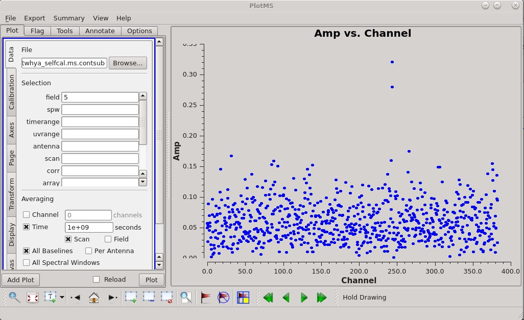
[[File:Imaging-tutorial-line-plotms-2_6.5.4.jpg|thumb|<caption>Figure 2: A plot of amplitude vs. channel number, after continuum subtraction. Note that because the amplitude is positive definite, you don't expect the line-free channels to go entirely down to zero. They should just | [[File:Imaging-tutorial-line-plotms-2_6.5.4.jpg|thumb|<caption>Figure 2: A plot of amplitude vs. channel number, after continuum subtraction. Note that because the amplitude is positive definite, you don't expect the line-free channels to go entirely down to zero. They should just | ||
average to a very small value that reflects the noise.</caption>]] | average to a very small value that reflects the noise.</caption>]] | ||
<source lang="python"> | <source lang="python"> | ||
| Line 136: | Line 131: | ||
In addition, the [https://help.almascience.org/kb/articles/what-changes-were-made-to-the-psf-beam-fitting-algorithm-in-casa-6 beam-fitting] algorithm has been updated, starting in CASA 6.2. | In addition, the [https://help.almascience.org/kb/articles/what-changes-were-made-to-the-psf-beam-fitting-algorithm-in-casa-6 beam-fitting] algorithm has been updated, starting in CASA 6.2. | ||
Otherwise, this {{tclean_6.5.4}} will resemble our previous calls when we imaged the continuum. | Otherwise, this {{tclean_6.5.4}} will resemble our previous calls when we imaged the continuum. | ||
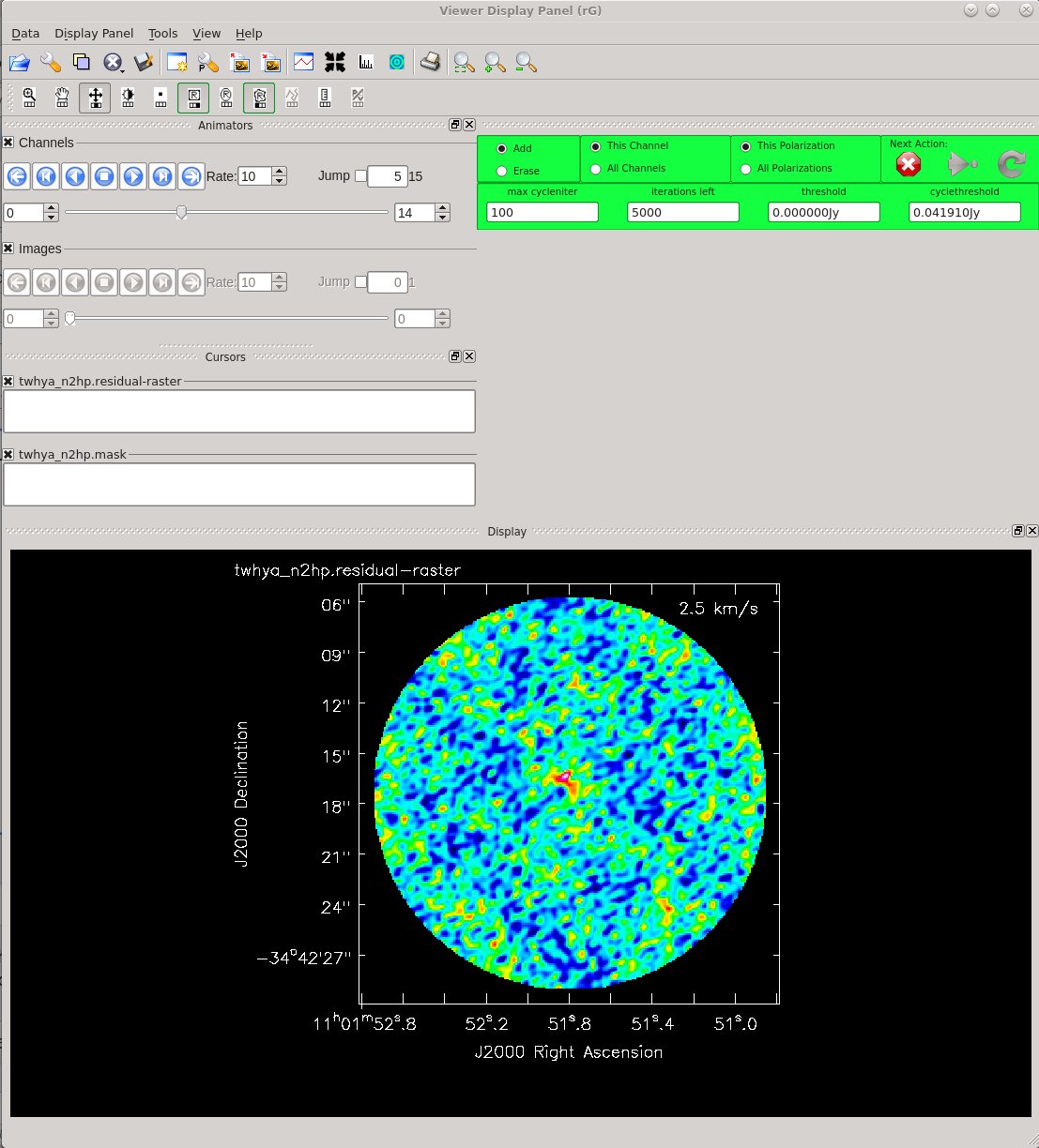
[[File:Imaging-tutorial-line-clean_6.5.4.jpg|thumb|<caption>Figure 3: Here we show the tclean viewer, after using the tape deck control to step up to channel 5, which shows some line emission.</caption>]] | [[File:Imaging-tutorial-line-clean_6.5.4.jpg|thumb|<caption>Figure 3: Here we show the tclean viewer, after using the tape deck control to step up to channel 5, which shows some line emission.</caption>]] | ||
<source lang="python"> | <source lang="python"> | ||
| Line 159: | Line 152: | ||
imsize = [250, 250], | imsize = [250, 250], | ||
cell = '0.1arcsec', | cell = '0.1arcsec', | ||
weighting = 'briggsbwtaper', | weighting = 'briggsbwtaper', | ||
robust = 0.5, | robust = 0.5, | ||
| Line 182: | Line 174: | ||
The output of the {{tclean_6.5.4}} task is a data cube. You can use CARTA to | The output of the {{tclean_6.5.4}} task is a data cube. You can use CARTA to | ||
inspect the cube, plot spectra, estimate the noise, and overlay this | inspect the cube, plot spectra, estimate the noise, and overlay this | ||
result with the earlier continuum image. | result with the earlier continuum image. If you are using NRAO machines, you can navigate to your working directory in a terminal, and then type: | ||
<source lang="bash"> | |||
# In bash | |||
carta --no_browser | |||
</source> | |||
Copy the URL it returns and paste into a browser window to view your CARTA session. | |||
[[File:Imaging-tutorial-line-profile_6.5.4.jpg|thumb|<caption>Figure 4: Here we show a spectral line profile plotted using the spectral profiler tool in CARTA.</caption>]] | [[File:Imaging-tutorial-line-profile_6.5.4.jpg|thumb|<caption>Figure 4: Here we show a spectral line profile plotted using the spectral profiler tool in CARTA.</caption>]] | ||
CARTA gives you the capability to make spectral profile plots. Load the cube image and use the "Animator" tab to step through the channels. Then use the drawing tools at the top to draw a box or ellipse or polygon around a region of interest, or set a single point using the "point marking" button to get a spectrum from a cut through a single pixel on the image. To get the spectrum, click the spectral profiler tool, highlighted with a red box in Figure 4. The spectrum shown is from a small region centered on one of the bright lobes of emission in channel 6. | CARTA gives you the capability to make spectral profile plots. Load the cube image and use the "Animator" tab to step through the channels. Then use the drawing tools at the top to draw a box or ellipse or polygon around a region of interest, or set a single point using the "point marking" button to get a spectrum from a cut through a single pixel on the image. To get the spectrum, click the spectral profiler tool, highlighted with a red box in Figure 4. The spectrum shown is from a small region centered on one of the bright lobes of emission in channel 6. | ||
Latest revision as of 20:16, 15 August 2024
About this Guide
Last checked on CASA Version 6.5.4
This guide features CARTA, the “Cube Analysis and Rendering Tool for Astronomy,” which is the new NRAO visualization tool for images and cubes. The CASA viewer (imview) has not been maintained for a few years and will be removed from future versions of CASA. We strongly recommend using CARTA, as it provides a much more efficient, stable, and feature rich user experience. A comparison of the CASA viewer and CARTA, as well as instructions on how to use CARTA at NRAO, is provided in the CARTA section of the CASA docs.
This lesson steps you through imaging of spectral lines.
We start here with the self-calibrated data from the previous tutorial. We could just as easily begin with the non self-calibrated data, but we would not then benefit from the improvements that the self calibration provided.
If you have not completed the previous tutorial, you'll need the self-calibrated data. You can download the full package for these First Look tutorials following the instructions at First_Look_at_Imaging_CASA_6.5.4 Guide for instructions. The full package contains twhya_selfcal.ms.tar, or you can download twhya_selfcal.ms.tar separately at https://bulk.cv.nrao.edu/almadata/public/ALMA_firstlooks/twhya_selfcal.ms.tar .
Note that it often makes good sense to self-calibrate on the continuum source, even when the main science goal is to image spectral line emission. This is especially true when the continuum is bright and not overly complex. Sometimes, though, it can make better sense to self-calibrate on a spectral line, and apply those solutions to the entire data set. For now, we will apply the continuum self-cal solutions to our spectral line data to optimize our spectral line images.
First, copy the self-calibrated measurement set to the current directory. This measurement set contains both spectral line and continuum data for our science target. Note that if you would like to use your own self-calibrated measurement set from the previous tutorial here, you will need to change the filename in the commands from 'twhya_selfcal.ms' to your best result (i.e., 'twhya_selfcal_4.ms') throughout this tutorial.
If you do not want to use your own self-calibrated data, and you downloaded the full package:
# In CASA - comment these two lines out of extracted script if you created your own selfcal.ms
os.system('rm -rf twhya_selfcal.ms')
os.system('tar -xvf ../working/twhya_selfcal.ms.tar')
The untarred measurement set will be automatically placed in your current directory, which can be verified with an "ls" command.
Continuum subtraction
Our first step is to remove the continuum emission from the UV data. Here, continuum emission means broadband emission that spans all spectral channels. The continuum may have some mild frequency dependence, and that's OK. The cleanest way to do the continuum subtraction is to operate on the UV data, fitting the amplitudes using only those spectral channels that are free from spectral line emission. We will do so using the CASA task uvcontsub.
The main subtlety in the UV continuum subtraction is that we want to be sure to fit the continuum using only channels that contain mostly continuum (and not line) emission. To this end, the first thing that we will do is plot the integrated spectrum of the science target using the plotms task. We specify the science source (field 5) and plot the amplitude as a function of channel number, averaging the data over time. (The parameter avgscan=True tells CASA to allow time averaging across scans.)

# In CASA
plotms(vis='twhya_selfcal.ms',
       xaxis='channel',
       yaxis='amp',
       field='5',
       avgspw=False,
       avgtime='1e9',
       avgscan=True,
       avgbaseline=True,
       showgui = True)
Inside the plotms tabs, you can toggle the axis to frequency and then back to channel - the N2H+ line is at 372.67249 GHz and you can see that there are several high amplitudes around channel 250 representing a weak but still visible spectral line. The rest of the spectrum seems reasonably clear for measuring the continuum. To be sure that we exclude all spectral line emission, let's avoid channels 240-280 in our continuum fit.
*NOTE* The uvcontsub task in CASA 6.5.4 is different than the uvcontsub in previous versions. The input parameters have changed, and this new task currently does not support combining spws for fitting. If you need this functionality, you can use the old version of uvcontsub by calling uvcontsub_old.
In our call to uvcontsub, we specify the line-free regions by setting fitspec='0:0~239;281~383'. In this case we'll fit only a constant amplitude (flat) continuum by setting the fitorder to 0. We target only field '5', the science source. We want to write out the continuum-subtracted measurement set to "twhya_selfcal.ms.contsub".
On a larger ALMA dataset, this step may take some time depending on your computing resources!
# In CASA
os.system('rm -rf twhya_selfcal.ms.contsub')
uvcontsub(vis = 'twhya_selfcal.ms',
          field = '5',
          fitspec = '0:0~239;281~383',
          fitorder = 0,
          outputvis='twhya_selfcal.ms.contsub')
The output is a continuum-subtracted UV data set that has the file extension ".contsub". We can now plot that using plotms, similar to what we did before, and look at the spectrum, which should now contain only the spectral line. Note that uvcontsub preserves the field number, unlike uvcontsub_old.

# In CASA
plotms(vis='twhya_selfcal.ms.contsub',
       xaxis='channel',
       yaxis='amp',
       field='5',
       avgspw=False,
       avgtime='1e9',
       avgscan=True,
       avgbaseline=True,
       showgui = True)
The continuum subtraction looks reasonably good. We'll see better when we image the cube.
Imaging the spectral line
Line imaging is like continuum imaging with (as you would expect) the additional dimension of spectral information. In the call to tclean, we now need to set specmode="cube". Further, we need to specify the third axis onto which the data will be gridded by setting appropriate values (and units) for the start, width, and nchan parameters. This third axis can be specified in units of channel, velocity, or frequency. Any of these choices would be valid for these data. Here, we image 15 channels in the output data cube, each 0.5 km/s in width, starting at 0 km/s in the LSRK reference frame by setting start="0.0km/s", nchan=15, and width="0.5km/s". The velocity is defined relative to the N2H+ rest frequency, which can be looked up in splatalogue.
Set the N2H+ rest frequency in a python variable as follows:
# In CASA
restfreq = '372.67249GHz'
Next we will use tclean to make the cube, targeting the continuum-subtracted data. Set field to '5' and spw to '0' (the only options in this data set), and use specmode="cube" with 15 channels of 0.5 km/s starting at 0.0 km/s defined in the LSRK frame (a common frame for Galactic and extragalactic work). We also set restoringbeam='common' to ensure a constant beam size for each plane in the cube. Weighting has been changed to 'briggsbwtaper'. This is a new weighting scheme available starting in CASA 6.2. See Imaging Algorithms for more information. In addition, the beam-fitting algorithm has been updated, starting in CASA 6.2. Otherwise, this tclean will resemble our previous calls when we imaged the continuum.

# In CASA
os.system('rm -rf twhya_n2hp.*')
tclean(vis = 'twhya_selfcal.ms.contsub',
       imagename = 'twhya_n2hp',
       field = '5',
       spw = '0',
       specmode = 'cube',
       perchanweightdensity=True,
       nchan = 15,
       start = '0.0km/s',
       width = '0.5km/s',
       outframe = 'LSRK',
       restfreq = restfreq,
       deconvolver= 'hogbom',
       gridder = 'standard',
       imsize = [250, 250],
       cell = '0.1arcsec',
       weighting = 'briggsbwtaper',
       robust = 0.5,
       restoringbeam='common',
       interactive = True,
       niter=5000)
We specified interactive mode, so the clean GUI will come up. When it does, step through the channels in the cube using the tape deck controls. We see emission over a few channels near the center of the cube. Notice the location of the emission shifts from channel to channel -- Cool! This is showing velocity structure from the rotating disk!
Since the line emission has fairly low signal-to-noise, we don't expect cleaning to make a dramatic improvement here. But, let's give it a shot to try to improve the image. For spectral cubes, it's possible to specify a clean mask individually for each velocity channel, or you can specify a single mask that gets applied to all channels. There is a button at the top of the tclean GUI that toggles between these options. Both are viable approaches. For a high fidelity telescope like ALMA it's often (but not always) fine to use a single mask across all channels. Try interactively drawing a clean mask as you did previously in the CASA guide for continuum imaging. Select either the button to clean only "This channel" or apply the clean mask to all channels by selecting the "All channels" button below it. Then clean for 100 iterations or so until the maximum of the residuals inside the clean box is comparable to the surrounding noise. To finish, close the clean window by clicking the red "X."
The output of the tclean task is a data cube. You can use CARTA to inspect the cube, plot spectra, estimate the noise, and overlay this result with the earlier continuum image. If you are using NRAO machines, you can navigate to your working directory in a terminal, and then type:
# In bash
carta --no_browser
Copy the URL it returns and paste into a browser window to view your CARTA session.

CARTA gives you the capability to make spectral profile plots. Load the cube image and use the "Animator" tab to step through the channels. Then use the drawing tools at the top to draw a box or ellipse or polygon around a region of interest, or set a single point using the "point marking" button to get a spectrum from a cut through a single pixel on the image. To get the spectrum, click the spectral profiler tool, highlighted with a red box in Figure 4. The spectrum shown is from a small region centered on one of the bright lobes of emission in channel 6.
Primary beam correction
As with continuum imaging, the line data cubes produced by CASA do not have the primary beam correction by default. Remember that to form an astronomically correct image of the sky, the output of tclean needs to be divided by this primary beam (or, in the case of mosaics, the combination of primary beam patterns used to make the mosaic). For final calculations you will therefore want to produce a primary beam-corrected version of your cube. You can create the primary beam-corrected cube in tclean by setting the parameter pbcor = True. This will produce an additional file with the extension .image.pbcor, which is the cleaned cube corrected for the primary beam.
If you've already cleaned your data and don't want to rerun tclean, CASA stores the primary beam information needed to make this correction in the file with the .pb extension. The CASA task impbcor can be used to combine the .pb image with the output image from tclean to produce a primary-beam corrected image. First remove the old primary beam corrected image if it exists:
# In CASA
os.system('rm -rf twhya_n2hp.pbcor.image')
Now correct the image:
# In CASA
impbcor(imagename='twhya_n2hp.image',
        pbimage='twhya_n2hp.pb',
        outfile='twhya_n2hp.pbcor.image')