Jupiter: continuum polarization calibration 6.4.1: Difference between revisions
No edit summary |
|||
| (31 intermediate revisions by the same user not shown) | |||
| Line 3: | Line 3: | ||
| style="background: red; color: white;" | '''DISCLAIMER''' | | style="background: red; color: white;" | '''DISCLAIMER''' | ||
|- | |- | ||
| This is an advanced reference guide to calibration and imaging of pre-upgrade VLA polarimetric data with CASA 6.4.1. If you are a | | This is an advanced reference guide to calibration and imaging of pre-upgrade VLA polarimetric data with CASA 6.4.1. If you are a beginner or novice user, please consult the relevant [https://casaguides.nrao.edu/index.php/Karl_G._Jansky_VLA_Tutorials CASA guides] first. | ||
|} | |} | ||
== Data Download | == Overview, Data Download, & Import == | ||
'''Overview''' | |||
This CASA guide discusses how to set the flux scale for calibration of an archival VLA multi-band data set, taken in D-configuration (15 April 1999), with a resolution of around 14 arcsec. The original observation included several planets and observing bands. This guide will focus on Jupiter and its respective calibrators in C-band (6cm). | This CASA guide discusses how to set the flux scale for calibration of an archival VLA multi-band data set, taken in D-configuration (15 April 1999), with a resolution of around 14 arcsec. The original observation included several planets and observing bands. This guide will focus on Jupiter and its respective calibrators in C-band (6cm). | ||
''' | We would like to note that the CASAviewer has not been maintained for a few years and will be removed from future versions of CASA. The NRAO replacement visualization tool for images and cubes is CARTA, the “Cube Analysis and Rendering Tool for Astronomy”. It is available from the '''[https://cartavis.org/ CARTA]''' website. We strongly recommend to use CARTA, as it provides a much more efficient, stable, and feature rich user experience. A comparison of the CASAviewer and CARTA, as well as instructions on how to use CARTA at NRAO is provided in the respective section of '''[https://casadocs.readthedocs.io/en/stable/notebooks/carta.html CASA docs]'''. This tutorial shows Figures generated with CARTA for visualization. | ||
(Note, all CASA guides are meant to be used with monolithic CASA and not pip-wheel, because the GUIs are not necessarily validated.) | |||
'''Data Download Options''' | |||
The data set for this tutorial can be downloaded from the '''[https://data.nrao.edu NRAO Archive Access Tool (AAT)]''' by searching on '''FLUX99''' in the top search bar. You will see one data set to download, FLUX99_1_51283.96221_51284.96001.exp. There are two approaches to downloading this data set. Since this is a very small data set, it should only take about a minute. | The data set for this tutorial can be downloaded from the '''[https://data.nrao.edu NRAO Archive Access Tool (AAT)]''' by searching on '''FLUX99''' in the top search bar. You will see one data set to download, FLUX99_1_51283.96221_51284.96001.exp. There are two approaches to downloading this data set. Since this is a very small data set, it should only take about a minute. | ||
| Line 20: | Line 28: | ||
If you need help with this step, please contact us through the '''[https://help.nrao.edu NRAO Science Helpdesk]''' under the '''VLA/VLBA Archive and Data Retrieval''' department. | If you need help with this step, please contact us through the '''[https://help.nrao.edu NRAO Science Helpdesk]''' under the '''VLA/VLBA Archive and Data Retrieval''' department. | ||
The operator/observing log can be found online at the '''[http://www.vla.nrao.edu/astro/archive/obslogs/ VLA Archive: Observing Logs]''' webpage. Select April 1999 and then select View. You will see a long list of all the observing logs from April 1999, use the web browser to search on FLUX99. You will find four logs, since a new log was created each time there was an operator shift change during an observation. | |||
| Line 33: | Line 44: | ||
casa -r 6.4.1-12-pipeline-2022.2.0.64 | casa -r 6.4.1-12-pipeline-2022.2.0.64 | ||
</source> | </source> | ||
'''Importing Data''' | '''Importing Data''' | ||
| Line 794: | Line 806: | ||
########################################## | ########################################## | ||
</pre> | </pre> | ||
[[Image:CASA6.4.1-plotants.png|thumb|Figure 1: plotants]] | |||
Next, we will use '''[https://casadocs.readthedocs.io/en/v6.4.1/api/tt/casatasks.manipulation.split.html?highlight=split split]''' to split out the following into a new MS. | Next, we will use '''[https://casadocs.readthedocs.io/en/v6.4.1/api/tt/casatasks.manipulation.split.html?highlight=split split]''' to split out the following into a new MS. | ||
| Line 810: | Line 824: | ||
<source lang="python"> | <source lang="python"> | ||
# Figure 1 | |||
plotants(vis='jupiter6cm.demo.ms', figfile='jupiter6cm.demo.ant.png') | plotants(vis='jupiter6cm.demo.ms', figfile='jupiter6cm.demo.ant.png') | ||
</source> | </source> | ||
| Line 816: | Line 831: | ||
== Data Inspection and Flagging == | == Data Inspection and Flagging == | ||
[[Image:CASA6.4.1-ampvUVdist.png|thumb|Figure 2: plotms Amplitude vs. UVdist colorized by spw (vis='jupiter6cm.demo.ms')]] | |||
In this section we present two methods of flagging the data: | In this section we present two methods of flagging the data: | ||
| Line 826: | Line 843: | ||
<source lang="python"> | <source lang="python"> | ||
# Figure 2 | |||
plotms(vis='jupiter6cm.demo.ms', selectdata=True, field='1331+305', correlation='RR,LL', xaxis='uvdist', yaxis='amp') | plotms(vis='jupiter6cm.demo.ms', selectdata=True, field='1331+305', correlation='RR,LL', xaxis='uvdist', yaxis='amp') | ||
</source> | </source> | ||
| Line 877: | Line 895: | ||
=== Initial Gain Calibration === | === Initial Gain Calibration === | ||
[[Image:CASA6.4.1-ampvtime.png|thumb|Figure | [[Image:CASA6.4.1-ampvtime.png|thumb|Figure 3: plotms Amplitude vs. Time (vis='jupiter6cm.demo.G').]] | ||
[[Image:CASA6.4.1-phsvtime.png|thumb|Figure | [[Image:CASA6.4.1-phsvtime.png|thumb|Figure 4: plotms Phase vs. Time (vis='jupiter6cm.demo.G').]] | ||
[[Image:CASA6.4.1-gainampvtime.png|thumb|Figure | [[Image:CASA6.4.1-gainampvtime.png|thumb|Figure 5: plotms Gain Amp vs. Time (plotfile='jupiter6cm.demo.Gflx.amp.png').]] | ||
[[Image:CASA6.4.1-gainphasevtime.png|thumb|Figure | [[Image:CASA6.4.1-gainphasevtime.png|thumb|Figure 6: plotms Gain Phase vs. Time (plotfile='jupiter6cm.demo.Gflx.phase.png').]] | ||
At this stage the data have an overall flux density scaling determined, but full gain solutions aren't there yet. The relevant task is '''[https://casadocs.readthedocs.io/en/v6.4.1/api/tt/casatasks.calibration.gaincal.html?highlight=gaincal gaincal]''' (analogous to the AIPS task CALIB). '''[https://casadocs.readthedocs.io/en/v6.4.1/api/tt/casatasks.calibration.gaincal.html?highlight=gaincal Gaincal]''' will produce a separate table with solutions, and we will use appropriate extensions to keep track of the different tables and their corresponding solutions (e.g., gain curve table = .gc). | At this stage the data have an overall flux density scaling determined, but full gain solutions aren't there yet. The relevant task is '''[https://casadocs.readthedocs.io/en/v6.4.1/api/tt/casatasks.calibration.gaincal.html?highlight=gaincal gaincal]''' (analogous to the AIPS task CALIB). '''[https://casadocs.readthedocs.io/en/v6.4.1/api/tt/casatasks.calibration.gaincal.html?highlight=gaincal Gaincal]''' will produce a separate table with solutions, and we will use appropriate extensions to keep track of the different tables and their corresponding solutions (e.g., gain curve table = .gc). | ||
| Line 898: | Line 916: | ||
# And check the solutions | # And check the solutions | ||
# Figure | # Figure 3: | ||
plotms(vis='jupiter6cm.demo.G', xaxis='time', yaxis='amp', gridrows=3, gridcols=3, iteraxis='antenna') | plotms(vis='jupiter6cm.demo.G', xaxis='time', yaxis='amp', gridrows=3, gridcols=3, iteraxis='antenna') | ||
# Figure | # Figure 4: | ||
plotms(vis='jupiter6cm.demo.G', xaxis='time', yaxis='phase', plotrange=[-1,-1,-200,200], gridrows=3, gridcols=3, iteraxis='antenna') | plotms(vis='jupiter6cm.demo.G', xaxis='time', yaxis='phase', plotrange=[-1,-1,-200,200], gridrows=3, gridcols=3, iteraxis='antenna') | ||
</source> | </source> | ||
| Line 937: | Line 955: | ||
</source> | </source> | ||
* Figure | * Figure 5 (jupiter6cm.demo.Gflx.amp.png) will show two data points: the value at 1.0 is from 3C286 and the value at 0.42 is the complex gain calibrator. The reason 3C286 is 1.0 is because it is used as the reference and the complex gain calibrator is the flux ratio referenced to 3C286, which is assumed 1.0. In this observation, 3C286 was used as the flux density reference. | ||
* Figure | * Figure 6 (jupiter6cm.demo.Gflx.phase.png) will show two data points at zero (plotted on top of each other). Since we are just scaling amplitudes, we are not expecting the phases to be modified by this calibration table, thus the phases are zero. | ||
=== Polarization Calibration === | === Polarization Calibration === | ||
| Line 947: | Line 965: | ||
==== Set the Polarization Model ==== | ==== Set the Polarization Model ==== | ||
First, set the polarization model for the polarized position-angle calibrator (here 1331+305=3C286 which is also our primary flux calibrator). For polarization properties of your primary polarization calibrator see the '''[https://science.nrao.edu/facilities/vla/docs/manuals/obsguide/modes/pol | First, set the polarization model for the polarized position-angle calibrator (here 1331+305=3C286 which is also our primary flux calibrator). For polarization properties of your primary polarization calibrator see the '''[https://science.nrao.edu/facilities/vla/docs/manuals/obsguide/modes/pol Polarimetry]''' section of the '''[https://go.nrao.edu/vla-obs VLA Observing Guide]'''. | ||
<source lang="python"> | <source lang="python"> | ||
| Line 976: | Line 994: | ||
==== Solve for the Leakage Terms (D terms) ==== | ==== Solve for the Leakage Terms (D terms) ==== | ||
[[Image:CASA6.4.1-ampvant1.png|thumb|Figure | [[Image:CASA6.4.1-ampvant1.png|thumb|Figure 7: plotms Gain Amp vs. Antenna1 (plotfile='jupiter6cm.demo.D.amp.png').]] | ||
[[Image:CASA6.4.1-phsvant1.png|thumb|Figure | [[Image:CASA6.4.1-phsvant1.png|thumb|Figure 8: plotms Gain Phase vs. Antenna1 (plotfile='jupiter6cm.demo.D.phase.png').]] | ||
[[Image:CASA6.4.1-SNRvant1.png|thumb|Figure | [[Image:CASA6.4.1-SNRvant1.png|thumb|Figure 9: plotms SNR vs. Antenna1 (plotfile='jupiter6cm.demo.D.snr.png').]] | ||
In this step we solve for the instrumental polarization. Solving for polarization leakage on 0137+331, we will assume our calibrator has unknown polarization. | In this step we solve for the instrumental polarization. Solving for polarization leakage on 0137+331, we will assume our calibrator has unknown polarization. | ||
| Line 992: | Line 1,010: | ||
<source lang="python"> | <source lang="python"> | ||
# Figure | # Figure 7: | ||
plotms(vis='jupiter6cm.demo.D', xaxis='antenna1', yaxis='amp', showgui=True, plotfile='jupiter6cm.demo.D.amp.png') | plotms(vis='jupiter6cm.demo.D', xaxis='antenna1', yaxis='amp', showgui=True, plotfile='jupiter6cm.demo.D.amp.png') | ||
# Figure | # Figure 8: | ||
plotms(vis='jupiter6cm.demo.D', xaxis='antenna1', yaxis='phase', plotrange=[-1,-1,-200,200], showgui=True, plotfile='jupiter6cm.demo.D.phase.png') | plotms(vis='jupiter6cm.demo.D', xaxis='antenna1', yaxis='phase', plotrange=[-1,-1,-200,200], showgui=True, plotfile='jupiter6cm.demo.D.phase.png') | ||
# Figure | # Figure 9: | ||
plotms(vis='jupiter6cm.demo.D', xaxis='antenna1', yaxis='snr', showgui=True, plotfile='jupiter6cm.demo.D.snr.png') | plotms(vis='jupiter6cm.demo.D', xaxis='antenna1', yaxis='snr', showgui=True, plotfile='jupiter6cm.demo.D.snr.png') | ||
</source> | </source> | ||
| Line 1,027: | Line 1,045: | ||
=== Apply the Calibration === | === Apply the Calibration === | ||
Now that we have derived all the calibration solutions and saved them in the tables of multiple extensions, we need to apply them to the actual data. The '''[https://casadocs.readthedocs.io/en/v6.4.1/api/tt/casatasks.calibration.applycal.html?highlight=applycal applycal]''' task commands will apply the solution tables to the DATA and write a new column CORRECTED_DATA as it is standard for CASA. Important: make sure you set <tt>parang=True</tt>. | Now that we have derived all the calibration solutions and saved them in the tables of multiple extensions, we need to apply them to the actual data. The '''[https://casadocs.readthedocs.io/en/v6.4.1/api/tt/casatasks.calibration.applycal.html?highlight=applycal applycal]''' task commands will apply the solution tables to the DATA column and write a new column CORRECTED_DATA as it is standard for CASA. Important: make sure you set <tt>parang=True</tt>. | ||
<source lang="python"> | <source lang="python"> | ||
| Line 1,048: | Line 1,066: | ||
== Initial Imaging (Stokes I) == | == Initial Imaging (Stokes I) == | ||
[[Image:CARTA3.0.0-jupiter-clean1-rms.png|thumb|Figure | [[Image:CARTA3.0.0-jupiter-clean1-rms.png|thumb|Figure 10: Annotated screen shot of jupiter6cm.demo.JUPITER.I.clean1 in CARTA.]] | ||
Next we will image and clean the Jupiter data. In this step we will self-calibrate, therefore in the initial imaging we will not clean too deeply and we will save the model in the MS data (with the use of parameter <tt>savemodel</tt> in '''[https://casadocs.readthedocs.io/en/v6.4.1/api/tt/casatasks.imaging.tclean.html?highlight=tclean tclean]'''). | Next we will image and clean the Jupiter data. In this step we will self-calibrate, therefore in the initial imaging we will not clean too deeply and we will save the model in the MS data (with the use of parameter <tt>savemodel</tt> in '''[https://casadocs.readthedocs.io/en/v6.4.1/api/tt/casatasks.imaging.tclean.html?highlight=tclean tclean]'''). | ||
| Line 1,073: | Line 1,091: | ||
# Near the top, select the Statistics Widget (tiny calculator icon). Here you will see the rms of the sky around Jupiter. These numbers will change as you move the box around the blank sky. | # Near the top, select the Statistics Widget (tiny calculator icon). Here you will see the rms of the sky around Jupiter. These numbers will change as you move the box around the blank sky. | ||
For an annotated visual example, refer to Figure | For an annotated visual example, refer to Figure 10. (Note, this session of CARTA is using the Dark mode theme found under View.) | ||
| Line 1,082: | Line 1,100: | ||
== Self-Calibration == | == Self-Calibration == | ||
[[Image:CASA6.4.1-ampvtime-ant.png|thumb|Figure | [[Image:CASA6.4.1-ampvtime-ant.png|thumb|Figure 11: plotms Gain Amp vs. Time per antenna (vis='jupiter6cm.demo.JUPITER.split.selfcal1').]] | ||
[[Image:CASA6.4.1-phsvtime-ant.png|thumb|Figure | [[Image:CASA6.4.1-phsvtime-ant.png|thumb|Figure 12: plotms Gain Phase vs. Time per antenna (vis='jupiter6cm.demo.JUPITER.split.selfcal1').]] | ||
[[Image:CARTA3.0.0-jupiter-clean1-2.png|thumb|Figure | [[Image:CARTA3.0.0-jupiter-clean1-2.png|thumb|Figure 13: Annotated screen shot of jupiter6cm.demo.JUPITER.I.clean1.image and jupiter6cm.demo.JUPITER.I.clean2.image in CARTA.]] | ||
In the self-calibration step we run '''[https://casadocs.readthedocs.io/en/v6.4.1/api/tt/casatasks.calibration.gaincal.html?highlight=gaincal gaincal]''' that will make use of the newly created MODEL column in our MS file. | In the self-calibration step we run '''[https://casadocs.readthedocs.io/en/v6.4.1/api/tt/casatasks.calibration.gaincal.html?highlight=gaincal gaincal]''' that will make use of the newly created MODEL column in our MS file. | ||
| Line 1,095: | Line 1,113: | ||
<source lang="python"> | <source lang="python"> | ||
# Figure | # Figure 11: | ||
plotms(vis='jupiter6cm.demo.JUPITER.split.selfcal1',xaxis='time',yaxis='amp',gridrows=2, gridcols=3, iteraxis='antenna') | plotms(vis='jupiter6cm.demo.JUPITER.split.selfcal1',xaxis='time',yaxis='amp',gridrows=2, gridcols=3, iteraxis='antenna') | ||
# Figure | # Figure 12: | ||
plotms(vis='jupiter6cm.demo.JUPITER.split.selfcal1',xaxis='time',yaxis='phase', gridrows=2, gridcols=3 ,iteraxis='antenna',plotrange=[-1,-1,-180,180]) | plotms(vis='jupiter6cm.demo.JUPITER.split.selfcal1',xaxis='time',yaxis='phase', gridrows=2, gridcols=3 ,iteraxis='antenna',plotrange=[-1,-1,-180,180]) | ||
</source> | </source> | ||
| Line 1,114: | Line 1,132: | ||
</source> | </source> | ||
Check the image statistics using '''CARTA'''. See Figure | Check the image statistics using '''CARTA'''. See Figure 13 for details. | ||
# Open both images: '''jupiter6cm.demo.JUPITER.I.clean1.image''' and '''jupiter6cm.demo.JUPITER.I.clean2.image'''. (Note, only one image can be opened at a time. After you have opened one, you will then need to select File -> Append Image to open another image | # Open both images: '''jupiter6cm.demo.JUPITER.I.clean1.image''' and '''jupiter6cm.demo.JUPITER.I.clean2.image'''. (Note, only one image can be opened at a time. After you have opened one, you will then need to select File -> Append Image to open another image.) | ||
# In the lower right under Image List, select XY and R (under Matching) for both images. This will allow you to manipulate the images simultaneously. | # In the lower right under Image List, select XY and R (under Matching) for both images. This will allow you to manipulate the images simultaneously. | ||
# Hover your mouse over one of the images to reveal the zoom icons. These will allow you to zoom in/out of the image. | # Hover your mouse over one of the images to reveal the zoom icons. These will allow you to zoom in/out of the image. | ||
| Line 1,125: | Line 1,143: | ||
== Full Stokes Imaging == | == Full Stokes Imaging == | ||
[[Image:CARTA3.0.0-skyRMS-IQUV.png|thumb|Figure | [[Image:CARTA3.0.0-skyRMS-IQUV.png|thumb|Figure 14: Stokes parameters in CARTA of jupiter6cm.demo.JUPITER.IQUV.clean.]] | ||
At this stage we will perform full Stokes imaging using '''[https://casadocs.readthedocs.io/en/v6.4.1/api/tt/casatasks.imaging.tclean.html?highlight=tclean tclean]''' to create an image of each Stokes parameter that we will later use to create polarized intensity and angle images. | At this stage we will perform full Stokes imaging using '''[https://casadocs.readthedocs.io/en/v6.4.1/api/tt/casatasks.imaging.tclean.html?highlight=tclean tclean]''' to create an image of each Stokes parameter that we will later use to create polarized intensity and angle images. | ||
| Line 1,133: | Line 1,151: | ||
</source> | </source> | ||
Inspect the quality of the cleaned image in '''CARTA''' (see Figure | Inspect the quality of the cleaned image in '''CARTA''' (see Figure 14). | ||
# Open '''jupiter6cm.demo.JUPITER.IQUV.clean.image''', | # Open '''jupiter6cm.demo.JUPITER.IQUV.clean.image''', | ||
# Create a box in a blank part of the sky next to Jupiter, | # Create a box in a blank part of the sky next to Jupiter, | ||
# Select the Statistics Widget, and select the Stokes parameter in the Polarization drop-down menu located in the statistics | # Select the Statistics Widget, and select the Stokes parameter in the Polarization drop-down menu located in the statistics window. | ||
Depending on how deeply you cleaned, you may reach rms values of about: | Depending on how deeply you cleaned, you may reach rms values of about: | ||
| Line 1,146: | Line 1,164: | ||
== Polarization Intensity and Position Angle Images == | == Polarization Intensity and Position Angle Images == | ||
[[Image:CARTA3.0.0- | [[Image:CARTA3.0.0-JUP-POLI-POLA-overlays.png|thumb|Figure 15: Jupiter (top left), polarization intensity (POLI) (top right) with contour overlay, and position angle (POLA) (bottom left) with vector overlay.]] | ||
Next, we will save each Stokes plane as separate images. We can use either the '''[https://casadocs.readthedocs.io/en/v6.4.1/api/tt/casatasks.analysis.imsubimage.html?highlight=imsubimage imsubimage]''' or '''[https://casadocs.readthedocs.io/en/v6.4.1/api/tt/casatasks.analysis.immath.html?highlight=immath immath]''' tasks to do so. | Next, we will save each Stokes plane as separate images. We can use either the '''[https://casadocs.readthedocs.io/en/v6.4.1/api/tt/casatasks.analysis.imsubimage.html?highlight=imsubimage imsubimage]''' or '''[https://casadocs.readthedocs.io/en/v6.4.1/api/tt/casatasks.analysis.immath.html?highlight=immath immath]''' tasks to do so. | ||
| Line 1,184: | Line 1,202: | ||
Again, check the statistics of these final images with '''[https://casadocs.readthedocs.io/en/stable/notebooks/carta.html CARTA]'''. | Again, check the statistics of these final images with '''[https://casadocs.readthedocs.io/en/stable/notebooks/carta.html CARTA]'''. | ||
See Figure | See Figure 15 to view Jupiter, POLI, and POLA images. Note, CARTA cannot yet overlay multiple images. However, it can overlay contours and vectors. | ||
| Line 1,197: | Line 1,215: | ||
<!--Last edited by Trent Seelig, 2019-08-27--> | <!--Last edited by Trent Seelig, 2019-08-27--> | ||
<!-- | <!--Last edited by Heidi Medlin, 2023/02/08 for CASA6.4.1 and CARTA3.0.0 (added many links & all screen shots)--> | ||
Latest revision as of 18:30, 9 February 2023
| DISCLAIMER |
| This is an advanced reference guide to calibration and imaging of pre-upgrade VLA polarimetric data with CASA 6.4.1. If you are a beginner or novice user, please consult the relevant CASA guides first. |
Overview, Data Download, & Import
Overview
This CASA guide discusses how to set the flux scale for calibration of an archival VLA multi-band data set, taken in D-configuration (15 April 1999), with a resolution of around 14 arcsec. The original observation included several planets and observing bands. This guide will focus on Jupiter and its respective calibrators in C-band (6cm).
We would like to note that the CASAviewer has not been maintained for a few years and will be removed from future versions of CASA. The NRAO replacement visualization tool for images and cubes is CARTA, the “Cube Analysis and Rendering Tool for Astronomy”. It is available from the CARTA website. We strongly recommend to use CARTA, as it provides a much more efficient, stable, and feature rich user experience. A comparison of the CASAviewer and CARTA, as well as instructions on how to use CARTA at NRAO is provided in the respective section of CASA docs. This tutorial shows Figures generated with CARTA for visualization.
(Note, all CASA guides are meant to be used with monolithic CASA and not pip-wheel, because the GUIs are not necessarily validated.)
Data Download Options
The data set for this tutorial can be downloaded from the NRAO Archive Access Tool (AAT) by searching on FLUX99 in the top search bar. You will see one data set to download, FLUX99_1_51283.96221_51284.96001.exp. There are two approaches to downloading this data set. Since this is a very small data set, it should only take about a minute.
- You may download the data set without logging in to your my.nrao.edu account. You will receive an email with instructions on how to retrieve the data.
- Or, login to the AAT with your my.nrao.edu username and password to make use of the NRAO lustre system. You will receive an email with instructions on how to retrieve the data directly or the path you chose for the data to be downloaded to. Note, you will need to have an active nm-account and a directory the AAT can write to (e.g., chmod 777 directory). Once the data has completed its download into your nm-account on lustre, you will need to cd into several directories starting with a string of numbers, then a *.exp/ directory, and then another *.exp/ directory, to then find the .exp file. For ease of use and finding again, you may want to consider moving this file into the top level of the directory you created to work with this file.
If you need help with this step, please contact us through the NRAO Science Helpdesk under the VLA/VLBA Archive and Data Retrieval department.
The operator/observing log can be found online at the VLA Archive: Observing Logs webpage. Select April 1999 and then select View. You will see a long list of all the observing logs from April 1999, use the web browser to search on FLUX99. You will find four logs, since a new log was created each time there was an operator shift change during an observation.
Running CASA
To choose which version of CASA you wish to use, type:
casa -ls
To run the CASA version used in this guide, type:
casa -r 6.4.1-12-pipeline-2022.2.0.64
Importing Data
CASA task importvla will read the .exp file format and create a CASA native measurement set (MS).
importvla(archivefiles='FLUX99_1_51283.96221_51284.96001.exp', vis='FLUX99.ms')
Use listobs to check the observation setup and print verbose summary of the observations to the CASA logger. The listfile input parameter is optional, but is good practice to print the listobs output to a text file for future reference.
listobs(vis='FLUX99.ms',listfile='FLUX99.txt')
The output of this task is fairly long, the abridged version is shown below since we will use this to determine which sources and spectral windows (spws) to split out for a simplified data set.
##########################################
##### Begin Task: listobs #####
Observer: unavailable Project: FLUX99
Observation: VLA
Data records: 9778860 Total elapsed time = 86210 seconds
Observed from 15-Apr-1999/23:06:06.7 to 16-Apr-1999/23:02:56.7 (TAI)
ObservationID = 0 ArrayID = 0
Date Timerange (TAI) Scan FldId FieldName nRows SpwIds Average Interval(s) ScanIntent
15-Apr-1999/23:06:06.7 - 23:13:30.0 1 0 0137+331 93366 [0,1] [3.33, 3.33]
23:13:36.7 - 23:15:00.0 2 0 0137+331 17550 [2,3] [3.33, 3.33]
23:15:16.7 - 23:16:10.0 3 0 0137+331 11232 [4,5] [3.33, 3.33]
23:19:06.7 - 23:20:20.0 4 0 0137+331 15444 [6,7] [3.33, 3.33]
23:20:36.7 - 23:21:30.0 5 0 0137+331 11232 [8,9] [3.33, 3.33]
23:21:46.7 - 23:22:50.0 6 0 0137+331 13338 [10,11] [3.33, 3.33]
23:23:06.7 - 23:24:10.0 7 0 0137+331 13338 [12,13] [3.33, 3.33]
23:38:26.7 - 23:48:00.0 8 1 0813+482 120744 [4,5] [3.33, 3.33]
23:48:06.7 - 23:49:30.0 9 1 0813+482 17550 [2,3] [3.33, 3.33]
23:49:36.7 - 23:50:50.0 10 1 0813+482 15444 [0,1] [3.33, 3.33]
23:51:06.7 - 23:52:00.0 11 1 0813+482 11232 [6,7] [3.33, 3.33]
23:53:36.7 - 23:55:20.0 12 2 0542+498 21762 [4,5] [3.33, 3.33]
23:55:26.7 - 23:56:50.0 13 2 0542+498 17550 [0,1] [3.33, 3.33]
23:56:56.7 - 23:58:00.0 14 2 0542+498 13338 [2,3] [3.33, 3.33]
16-Apr-1999/00:01:06.7 - 00:02:10.0 15 2 0542+498 13338 [6,7] [3.33, 3.33]
00:02:26.7 - 00:03:30.0 16 2 0542+498 13338 [8,9] [3.33, 3.33]
00:03:46.7 - 00:04:40.0 17 2 0542+498 11232 [10,11] [3.33, 3.33]
00:04:56.7 - 00:06:00.0 18 2 0542+498 13338 [12,13] [3.33, 3.33]
00:11:56.7 - 00:13:10.0 19 3 0521+166 15444 [2,3] [3.33, 3.33]
00:16:06.7 - 00:17:10.0 20 3 0521+166 13338 [6,7] [3.33, 3.33]
00:17:26.7 - 00:18:30.0 21 3 0521+166 13338 [8,9] [3.33, 3.33]
00:18:46.7 - 00:19:50.0 22 3 0521+166 13338 [10,11] [3.33, 3.33]
00:20:06.7 - 00:21:10.0 23 3 0521+166 13338 [12,13] [3.33, 3.33]
00:22:06.7 - 00:23:50.0 24 4 0437+296 21762 [4,5] [3.33, 3.33]
00:23:56.7 - 00:25:10.0 25 4 0437+296 15444 [0,1] [3.33, 3.33]
00:25:16.7 - 00:26:30.0 26 4 0437+296 15444 [2,3] [3.33, 3.33]
00:26:46.7 - 00:27:50.0 27 4 0437+296 13338 [6,7] [3.33, 3.33]
00:28:16.7 - 00:30:00.0 28 5 VENUS_0 21762 [4,5] [3.33, 3.33]
00:30:06.7 - 00:31:20.0 29 5 VENUS_0 15444 [2,3] [3.33, 3.33]
00:34:26.7 - 00:35:40.0 30 5 VENUS_0 15444 [6,7] [3.33, 3.33]
00:35:56.7 - 00:37:00.0 31 5 VENUS_0 13338 [8,9] [3.33, 3.33]
00:37:16.7 - 00:38:20.0 32 5 VENUS_0 13338 [10,11] [3.33, 3.33]
00:38:36.7 - 00:39:40.0 33 5 VENUS_0 13338 [12,13] [3.33, 3.33]
00:42:26.7 - 00:43:30.0 34 6 0319+415 13338 [8,9] [3.33, 3.33]
00:43:46.7 - 00:44:50.0 35 6 0319+415 13338 [10,11] [3.33, 3.33]
00:45:06.7 - 00:46:10.0 36 6 0319+415 13338 [12,13] [3.33, 3.33]
00:48:36.7 - 00:50:20.0 37 1 0813+482 21762 [4,5] [3.33, 3.33]
00:50:26.7 - 00:51:50.0 38 1 0813+482 17550 [2,3] [3.33, 3.33]
00:51:56.7 - 00:53:00.0 39 1 0813+482 13338 [0,1] [3.33, 3.33]
00:53:16.7 - 00:54:20.0 40 1 0813+482 13338 [6,7] [3.33, 3.33]
00:56:06.7 - 00:57:50.0 41 2 0542+498 21762 [4,5] [3.33, 3.33]
00:57:56.7 - 00:59:10.0 42 2 0542+498 15444 [0,1] [3.33, 3.33]
00:59:16.7 - 01:00:30.0 43 2 0542+498 15444 [2,3] [3.33, 3.33]
01:03:26.7 - 01:04:40.0 44 2 0542+498 15444 [6,7] [3.33, 3.33]
01:04:56.7 - 01:05:50.0 45 2 0542+498 11232 [8,9] [3.33, 3.33]
01:06:06.7 - 01:07:10.0 46 2 0542+498 13338 [10,11] [3.33, 3.33]
01:07:26.7 - 01:08:30.0 47 2 0542+498 13338 [12,13] [3.33, 3.33]
01:10:16.7 - 01:12:00.0 48 3 0521+166 21762 [4,5] [3.33, 3.33]
01:12:06.7 - 01:13:20.0 49 3 0521+166 15444 [0,1] [3.33, 3.33]
01:13:26.7 - 01:14:40.0 50 3 0521+166 15444 [2,3] [3.33, 3.33]
01:17:36.7 - 01:18:40.0 51 3 0521+166 13338 [6,7] [3.33, 3.33]
01:18:56.7 - 01:20:00.0 52 3 0521+166 13338 [8,9] [3.33, 3.33]
01:20:16.7 - 01:21:20.0 53 3 0521+166 13338 [10,11] [3.33, 3.33]
01:21:36.7 - 01:22:40.0 54 3 0521+166 13338 [12,13] [3.33, 3.33]
01:23:26.7 - 01:25:00.0 55 4 0437+296 19656 [4,5] [3.33, 3.33]
01:25:06.7 - 01:26:20.0 56 4 0437+296 15444 [0,1] [3.33, 3.33]
01:26:26.7 - 01:27:40.0 57 4 0437+296 15444 [2,3] [3.33, 3.33]
01:27:56.7 - 01:29:00.0 58 4 0437+296 13338 [6,7] [3.33, 3.33]
01:29:26.7 - 01:31:10.0 59 7 VENUS_1 21762 [4,5] [3.33, 3.33]
01:31:16.7 - 01:32:40.0 60 7 VENUS_1 17550 [2,3] [3.33, 3.33]
01:35:36.7 - 01:36:50.0 61 7 VENUS_1 15444 [6,7] [3.33, 3.33]
01:37:06.7 - 01:38:10.0 62 7 VENUS_1 13338 [8,9] [3.33, 3.33]
01:38:26.7 - 01:39:30.0 63 8 VENUS_2 13338 [10,11] [3.33, 3.33]
01:39:46.7 - 01:40:50.0 64 8 VENUS_2 13338 [12,13] [3.33, 3.33]
01:43:26.7 - 01:44:30.0 65 6 0319+415 13338 [8,9] [3.33, 3.33]
01:44:46.7 - 01:45:50.0 66 6 0319+415 13338 [10,11] [3.33, 3.33]
01:46:06.7 - 01:47:10.0 67 6 0319+415 13338 [12,13] [3.33, 3.33]
01:49:46.7 - 01:51:30.0 68 9 1411+522 21762 [4,5] [3.33, 3.33]
01:51:36.7 - 01:53:00.0 69 9 1411+522 17550 [0,1] [3.33, 3.33]
01:53:06.7 - 01:54:10.0 70 9 1411+522 13338 [2,3] [3.33, 3.33]
01:57:06.7 - 01:58:20.0 71 9 1411+522 15444 [6,7] [3.33, 3.33]
01:58:36.7 - 01:59:40.0 72 9 1411+522 13338 [8,9] [3.33, 3.33]
01:59:56.7 - 02:00:50.0 73 9 1411+522 11232 [10,11] [3.33, 3.33]
02:01:06.7 - 02:02:10.0 74 9 1411+522 13338 [12,13] [3.33, 3.33]
02:02:56.7 - 02:04:30.0 75 10 1331+305 19656 [4,5] [3.33, 3.33]
02:04:36.7 - 02:05:50.0 76 10 1331+305 15444 [0,1] [3.33, 3.33]
02:05:56.7 - 02:07:10.0 77 10 1331+305 15444 [2,3] [3.33, 3.33]
02:10:06.7 - 02:11:20.0 78 10 1331+305 15444 [6,7] [3.33, 3.33]
02:11:36.7 - 02:12:30.0 79 10 1331+305 11232 [8,9] [3.33, 3.33]
02:12:46.7 - 02:13:50.0 80 10 1331+305 13338 [10,11] [3.33, 3.33]
02:14:06.7 - 02:15:10.0 81 10 1331+305 13338 [12,13] [3.33, 3.33]
02:17:26.7 - 02:19:10.0 82 1 0813+482 21762 [4,5] [3.33, 3.33]
02:19:16.7 - 02:20:30.0 83 1 0813+482 15444 [2,3] [3.33, 3.33]
02:20:36.7 - 02:21:50.0 84 1 0813+482 15444 [0,1] [3.33, 3.33]
02:22:06.7 - 02:23:10.0 85 1 0813+482 13338 [6,7] [3.33, 3.33]
02:24:16.7 - 02:26:00.0 86 2 0542+498 21762 [4,5] [3.33, 3.33]
02:26:06.7 - 02:27:30.0 87 2 0542+498 17550 [0,1] [3.33, 3.33]
02:27:36.7 - 02:28:50.0 88 2 0542+498 15444 [2,3] [3.33, 3.33]
02:31:36.7 - 02:32:40.0 89 2 0542+498 13338 [6,7] [3.33, 3.33]
02:32:56.7 - 02:34:00.0 90 2 0542+498 13338 [8,9] [3.33, 3.33]
02:34:16.7 - 02:35:20.0 91 2 0542+498 13338 [10,11] [3.33, 3.33]
02:35:36.7 - 02:36:40.0 92 2 0542+498 13338 [12,13] [3.33, 3.33]
02:37:46.7 - 02:39:30.0 93 3 0521+166 21762 [4,5] [3.33, 3.33]
02:39:36.7 - 02:41:00.0 94 3 0521+166 17550 [0,1] [3.33, 3.33]
02:41:06.7 - 02:42:20.0 95 3 0521+166 15444 [2,3] [3.33, 3.33]
02:45:06.7 - 02:46:20.0 96 3 0521+166 15444 [6,7] [3.33, 3.33]
02:46:36.7 - 02:47:40.0 97 3 0521+166 13338 [8,9] [3.33, 3.33]
02:47:56.7 - 02:48:50.0 98 3 0521+166 11232 [10,11] [3.33, 3.33]
02:49:06.7 - 02:50:10.0 99 3 0521+166 13338 [12,13] [3.33, 3.33]
02:50:46.7 - 02:52:20.0 100 4 0437+296 19656 [4,5] [3.33, 3.33]
02:52:26.7 - 02:53:50.0 101 4 0437+296 17550 [0,1] [3.33, 3.33]
02:53:56.7 - 02:55:00.0 102 4 0437+296 13338 [2,3] [3.33, 3.33]
02:55:16.7 - 02:56:20.0 103 4 0437+296 13338 [6,7] [3.33, 3.33]
02:59:16.7 - 03:01:00.0 104 9 1411+522 21762 [4,5] [3.33, 3.33]
03:01:06.7 - 03:02:20.0 105 9 1411+522 15444 [0,1] [3.33, 3.33]
03:02:26.7 - 03:03:40.0 106 9 1411+522 15444 [2,3] [3.33, 3.33]
03:06:36.7 - 03:07:40.0 107 9 1411+522 13338 [6,7] [3.33, 3.33]
03:07:56.7 - 03:09:00.0 108 9 1411+522 13338 [8,9] [3.33, 3.33]
03:09:16.7 - 03:10:20.0 109 9 1411+522 13338 [10,11] [3.33, 3.33]
03:10:36.7 - 03:11:40.0 110 9 1411+522 13338 [12,13] [3.33, 3.33]
03:12:26.7 - 03:14:10.0 111 10 1331+305 21762 [4,5] [3.33, 3.33]
03:14:16.7 - 03:15:30.0 112 10 1331+305 15444 [0,1] [3.33, 3.33]
03:15:36.7 - 03:16:50.0 113 10 1331+305 15444 [2,3] [3.33, 3.33]
03:19:46.7 - 03:20:50.0 114 10 1331+305 13338 [6,7] [3.33, 3.33]
03:21:06.7 - 03:22:10.0 115 10 1331+305 13338 [8,9] [3.33, 3.33]
03:22:26.7 - 03:23:30.0 116 10 1331+305 13338 [10,11] [3.33, 3.33]
03:23:46.7 - 03:24:50.0 117 10 1331+305 13338 [12,13] [3.33, 3.33]
03:27:46.7 - 03:29:40.0 118 1 0813+482 23868 [4,5] [3.33, 3.33]
03:29:46.7 - 03:31:00.0 119 1 0813+482 15444 [2,3] [3.33, 3.33]
03:31:06.7 - 03:32:20.0 120 1 0813+482 15444 [0,1] [3.33, 3.33]
03:32:36.7 - 03:33:40.0 121 1 0813+482 13338 [6,7] [3.33, 3.33]
03:34:56.7 - 03:36:40.0 122 2 0542+498 21762 [4,5] [3.33, 3.33]
03:36:46.7 - 03:38:00.0 123 2 0542+498 15444 [0,1] [3.33, 3.33]
03:38:06.7 - 03:39:20.0 124 2 0542+498 15444 [2,3] [3.33, 3.33]
03:42:16.7 - 03:43:20.0 125 2 0542+498 13338 [6,7] [3.33, 3.33]
03:43:36.7 - 03:44:40.0 126 2 0542+498 13338 [8,9] [3.33, 3.33]
03:44:56.7 - 03:46:00.0 127 2 0542+498 13338 [10,11] [3.33, 3.33]
03:46:16.7 - 03:47:20.0 128 2 0542+498 13338 [12,13] [3.33, 3.33]
03:49:46.7 - 03:51:30.0 129 9 1411+522 21762 [4,5] [3.33, 3.33]
03:51:36.7 - 03:53:00.0 130 9 1411+522 17550 [0,1] [3.33, 3.33]
03:53:06.7 - 03:54:20.0 131 9 1411+522 15444 [2,3] [3.33, 3.33]
03:57:06.7 - 03:58:10.0 132 9 1411+522 13338 [6,7] [3.33, 3.33]
03:58:26.7 - 03:59:30.0 133 9 1411+522 13338 [8,9] [3.33, 3.33]
03:59:46.7 - 04:00:50.0 134 9 1411+522 13338 [10,11] [3.33, 3.33]
04:01:06.7 - 04:02:10.0 135 9 1411+522 13338 [12,13] [3.33, 3.33]
04:03:06.7 - 04:04:50.0 136 10 1331+305 21762 [4,5] [3.33, 3.33]
04:04:56.7 - 04:06:20.0 137 10 1331+305 17550 [0,1] [3.33, 3.33]
04:06:26.7 - 04:07:30.0 138 10 1331+305 13338 [2,3] [3.33, 3.33]
04:10:26.7 - 04:11:40.0 139 10 1331+305 15444 [6,7] [3.33, 3.33]
04:11:56.7 - 04:13:00.0 140 10 1331+305 13338 [8,9] [3.33, 3.33]
04:13:16.7 - 04:14:10.0 141 10 1331+305 11232 [10,11] [3.33, 3.33]
04:14:26.7 - 04:15:30.0 142 10 1331+305 13338 [12,13] [3.33, 3.33]
04:18:46.7 - 04:20:40.0 143 1 0813+482 23868 [4,5] [3.33, 3.33]
04:20:46.7 - 04:22:00.0 144 1 0813+482 15444 [2,3] [3.33, 3.33]
04:22:06.7 - 04:23:20.0 145 1 0813+482 15444 [0,1] [3.33, 3.33]
04:23:36.7 - 04:24:40.0 146 1 0813+482 13338 [6,7] [3.33, 3.33]
04:25:46.7 - 04:27:40.0 147 2 0542+498 23868 [4,5] [3.33, 3.33]
04:27:46.7 - 04:29:10.0 148 2 0542+498 17550 [0,1] [3.33, 3.33]
04:29:16.7 - 04:30:30.0 149 2 0542+498 15444 [2,3] [3.33, 3.33]
04:33:16.7 - 04:34:20.0 150 2 0542+498 13338 [6,7] [3.33, 3.33]
04:34:36.7 - 04:35:40.0 151 2 0542+498 13338 [8,9] [3.33, 3.33]
04:35:56.7 - 04:37:00.0 152 2 0542+498 13338 [10,11] [3.33, 3.33]
04:37:16.7 - 04:38:20.0 153 2 0542+498 13338 [12,13] [3.33, 3.33]
04:42:46.7 - 04:44:40.0 154 11 MARS_0 23868 [4,5] [3.33, 3.33]
04:44:50.0 - 04:46:00.0 155 12 MARS_1 14742 [2,3] [3.33, 3.33]
04:49:16.7 - 04:50:40.0 156 13 MARS_2 17550 [6,7] [3.33, 3.33]
04:50:56.7 - 04:52:00.0 157 13 MARS_2 13338 [8,9] [3.33, 3.33]
04:52:16.7 - 04:53:20.0 158 14 MARS_3 13338 [10,11] [3.33, 3.33]
04:53:36.7 - 04:54:40.0 159 14 MARS_3 13338 [12,13] [3.33, 3.33]
04:56:46.7 - 04:58:30.0 160 9 1411+522 21762 [4,5] [3.33, 3.33]
04:58:36.7 - 05:00:00.0 161 9 1411+522 17550 [0,1] [3.33, 3.33]
05:00:06.7 - 05:01:20.0 162 9 1411+522 15444 [2,3] [3.33, 3.33]
05:04:06.7 - 05:05:10.0 163 9 1411+522 13338 [6,7] [3.33, 3.33]
05:05:26.7 - 05:06:30.0 164 9 1411+522 13338 [8,9] [3.33, 3.33]
05:06:46.7 - 05:07:50.0 165 9 1411+522 13338 [10,11] [3.33, 3.33]
05:08:06.7 - 05:09:10.0 166 9 1411+522 13338 [12,13] [3.33, 3.33]
05:23:56.7 - 05:33:40.0 167 10 1331+305 122850 [4,5] [3.33, 3.33]
05:33:46.7 - 05:35:00.0 168 10 1331+305 15444 [0,1] [3.33, 3.33]
05:35:06.7 - 05:36:20.0 169 10 1331+305 15444 [2,3] [3.33, 3.33]
05:39:16.7 - 05:40:20.0 170 10 1331+305 13338 [6,7] [3.33, 3.33]
05:40:36.7 - 05:41:40.0 171 10 1331+305 13338 [8,9] [3.33, 3.33]
05:41:56.7 - 05:43:00.0 172 10 1331+305 13338 [10,11] [3.33, 3.33]
05:43:16.7 - 05:44:20.0 173 10 1331+305 13338 [12,13] [3.33, 3.33]
05:47:56.7 - 05:49:50.0 174 1 0813+482 23868 [4,5] [3.33, 3.33]
05:49:56.7 - 05:51:10.0 175 1 0813+482 15444 [2,3] [3.33, 3.33]
05:51:16.7 - 05:52:30.0 176 1 0813+482 15444 [0,1] [3.33, 3.33]
05:52:46.7 - 05:53:50.0 177 1 0813+482 13338 [6,7] [3.33, 3.33]
05:58:26.7 - 06:00:30.0 178 15 MARS_4 25974 [4,5] [3.33, 3.33]
06:00:36.7 - 06:02:00.0 179 16 MARS_5 17550 [2,3] [3.33, 3.33]
06:05:06.7 - 06:06:30.0 180 17 MARS_6 17550 [6,7] [3.33, 3.33]
06:06:46.7 - 06:08:00.0 181 17 MARS_6 15444 [8,9] [3.33, 3.33]
06:08:16.7 - 06:09:20.0 182 18 MARS_7 13338 [10,11] [3.33, 3.33]
06:09:36.7 - 06:10:30.0 183 18 MARS_7 11232 [12,13] [3.33, 3.33]
06:13:16.7 - 06:15:00.0 184 9 1411+522 21762 [4,5] [3.33, 3.33]
06:15:06.7 - 06:16:20.0 185 9 1411+522 15444 [0,1] [3.33, 3.33]
06:16:26.7 - 06:17:40.0 186 9 1411+522 15444 [2,3] [3.33, 3.33]
06:20:36.7 - 06:21:40.0 187 9 1411+522 13338 [6,7] [3.33, 3.33]
06:21:56.7 - 06:23:00.0 188 9 1411+522 13338 [8,9] [3.33, 3.33]
06:23:16.7 - 06:24:20.0 189 9 1411+522 13338 [10,11] [3.33, 3.33]
06:24:36.7 - 06:25:40.0 190 9 1411+522 13338 [12,13] [3.33, 3.33]
06:27:36.7 - 06:29:20.0 191 10 1331+305 21762 [4,5] [3.33, 3.33]
06:29:26.7 - 06:30:40.0 192 10 1331+305 15444 [0,1] [3.33, 3.33]
06:30:46.7 - 06:32:00.0 193 10 1331+305 15444 [2,3] [3.33, 3.33]
06:34:56.7 - 06:36:00.0 194 10 1331+305 13338 [6,7] [3.33, 3.33]
06:36:16.7 - 06:37:20.0 195 10 1331+305 13338 [8,9] [3.33, 3.33]
06:37:36.7 - 06:38:40.0 196 10 1331+305 13338 [10,11] [3.33, 3.33]
06:38:56.7 - 06:40:00.0 197 10 1331+305 13338 [12,13] [3.33, 3.33]
06:44:06.7 - 06:46:00.0 198 1 0813+482 23868 [4,5] [3.33, 3.33]
06:46:06.7 - 06:47:20.0 199 1 0813+482 15444 [2,3] [3.33, 3.33]
06:47:26.7 - 06:48:40.0 200 1 0813+482 15444 [0,1] [3.33, 3.33]
06:48:56.7 - 06:50:00.0 201 1 0813+482 13338 [6,7] [3.33, 3.33]
06:54:56.7 - 06:57:00.0 202 19 MARS_8 25974 [4,5] [3.33, 3.33]
06:57:06.7 - 06:58:20.0 203 20 MARS_9 15444 [2,3] [3.33, 3.33]
07:01:36.7 - 07:03:00.0 204 21 MARS_10 17550 [6,7] [3.33, 3.33]
07:03:16.7 - 07:04:20.0 205 22 MARS_11 13338 [8,9] [3.33, 3.33]
07:04:36.7 - 07:05:40.0 206 22 MARS_11 13338 [10,11] [3.33, 3.33]
07:05:56.7 - 07:07:00.0 207 23 MARS_12 13338 [12,13] [3.33, 3.33]
07:10:36.7 - 07:12:20.0 208 9 1411+522 21762 [4,5] [3.33, 3.33]
07:12:26.7 - 07:13:50.0 209 9 1411+522 17550 [0,1] [3.33, 3.33]
07:13:56.7 - 07:15:10.0 210 9 1411+522 15444 [2,3] [3.33, 3.33]
07:17:56.7 - 07:19:00.0 211 9 1411+522 13338 [6,7] [3.33, 3.33]
07:19:16.7 - 07:20:20.0 212 9 1411+522 13338 [8,9] [3.33, 3.33]
07:20:36.7 - 07:21:40.0 213 9 1411+522 13338 [10,11] [3.33, 3.33]
07:21:56.7 - 07:23:00.0 214 9 1411+522 13338 [12,13] [3.33, 3.33]
07:28:16.7 - 07:30:10.0 215 10 1331+305 23868 [4,5] [3.33, 3.33]
07:30:16.7 - 07:31:30.0 216 10 1331+305 15444 [0,1] [3.33, 3.33]
07:31:36.7 - 07:32:50.0 217 10 1331+305 15444 [2,3] [3.33, 3.33]
07:35:46.7 - 07:36:50.0 218 10 1331+305 13338 [6,7] [3.33, 3.33]
07:37:06.7 - 07:38:10.0 219 10 1331+305 13338 [8,9] [3.33, 3.33]
07:38:26.7 - 07:39:30.0 220 10 1331+305 13338 [10,11] [3.33, 3.33]
07:39:46.7 - 07:40:50.0 221 10 1331+305 13338 [12,13] [3.33, 3.33]
07:42:46.7 - 07:44:30.0 222 24 MARS_13 21762 [4,5] [3.33, 3.33]
07:44:36.7 - 07:46:00.0 223 24 MARS_13 17550 [2,3] [3.33, 3.33]
07:49:06.7 - 07:50:30.0 224 25 MARS_14 17550 [6,7] [3.33, 3.33]
07:50:46.7 - 07:52:00.0 225 25 MARS_14 15444 [8,9] [3.33, 3.33]
07:52:16.7 - 07:53:10.0 226 26 MARS_15 11232 [10,11] [3.33, 3.33]
07:53:26.7 - 07:54:30.0 227 26 MARS_15 13338 [12,13] [3.33, 3.33]
07:58:36.7 - 08:00:40.0 228 9 1411+522 25974 [4,5] [3.33, 3.33]
08:00:46.7 - 08:02:00.0 229 9 1411+522 15444 [0,1] [3.33, 3.33]
08:02:06.7 - 08:03:20.0 230 9 1411+522 15444 [2,3] [3.33, 3.33]
08:06:16.7 - 08:07:20.0 231 9 1411+522 13338 [6,7] [3.33, 3.33]
08:07:36.7 - 08:08:40.0 232 9 1411+522 13338 [8,9] [3.33, 3.33]
08:08:56.7 - 08:10:00.0 233 9 1411+522 13338 [10,11] [3.33, 3.33]
08:10:16.7 - 08:11:20.0 234 9 1411+522 13338 [12,13] [3.33, 3.33]
08:13:26.7 - 08:15:20.0 235 10 1331+305 23868 [4,5] [3.33, 3.33]
08:15:26.7 - 08:16:50.0 236 10 1331+305 17550 [0,1] [3.33, 3.33]
08:16:56.7 - 08:18:00.0 237 10 1331+305 13338 [2,3] [3.33, 3.33]
08:20:56.7 - 08:22:10.0 238 10 1331+305 15444 [6,7] [3.33, 3.33]
08:22:26.7 - 08:23:20.0 239 10 1331+305 11232 [8,9] [3.33, 3.33]
08:23:36.7 - 08:24:40.0 240 10 1331+305 13338 [10,11] [3.33, 3.33]
08:24:56.7 - 08:26:00.0 241 10 1331+305 13338 [12,13] [3.33, 3.33]
08:27:46.7 - 08:29:30.0 242 27 MARS_16 21762 [4,5] [3.33, 3.33]
08:29:36.7 - 08:30:50.0 243 27 MARS_16 15444 [2,3] [3.33, 3.33]
08:34:06.7 - 08:35:30.0 244 28 MARS_17 17550 [6,7] [3.33, 3.33]
08:35:46.7 - 08:36:50.0 245 28 MARS_17 13338 [8,9] [3.33, 3.33]
08:37:06.7 - 08:38:10.0 246 28 MARS_17 13338 [10,11] [3.33, 3.33]
08:38:26.7 - 08:39:30.0 247 29 MARS_18 13338 [12,13] [3.33, 3.33]
08:42:56.7 - 08:44:50.0 248 9 1411+522 23868 [4,5] [3.33, 3.33]
08:44:56.7 - 08:46:20.0 249 9 1411+522 17550 [0,1] [3.33, 3.33]
08:46:26.7 - 08:47:30.0 250 9 1411+522 13338 [2,3] [3.33, 3.33]
08:50:26.7 - 08:51:40.0 251 9 1411+522 15444 [6,7] [3.33, 3.33]
08:51:56.7 - 08:53:00.0 252 9 1411+522 13338 [8,9] [3.33, 3.33]
08:53:16.7 - 08:54:10.0 253 9 1411+522 11232 [10,11] [3.33, 3.33]
08:54:26.7 - 08:55:30.0 254 9 1411+522 13338 [12,13] [3.33, 3.33]
08:57:06.7 - 08:58:50.0 255 10 1331+305 21762 [4,5] [3.33, 3.33]
08:58:56.7 - 09:00:10.0 256 10 1331+305 15444 [0,1] [3.33, 3.33]
09:00:16.7 - 09:01:30.0 257 10 1331+305 15444 [2,3] [3.33, 3.33]
09:04:26.7 - 09:05:40.0 258 10 1331+305 15444 [6,7] [3.33, 3.33]
09:05:56.7 - 09:06:50.0 259 10 1331+305 11232 [8,9] [3.33, 3.33]
09:07:06.7 - 09:08:10.0 260 10 1331+305 13338 [10,11] [3.33, 3.33]
09:08:26.7 - 09:09:30.0 261 10 1331+305 13338 [12,13] [3.33, 3.33]
09:12:56.7 - 09:14:50.0 262 30 NGC7027 23868 [4,5] [3.33, 3.33]
09:14:56.7 - 09:16:20.0 263 30 NGC7027 17550 [2,3] [3.33, 3.33]
09:19:16.7 - 09:20:40.0 264 30 NGC7027 17550 [6,7] [3.33, 3.33]
09:20:56.7 - 09:22:10.0 265 30 NGC7027 15444 [8,9] [3.33, 3.33]
09:22:26.7 - 09:23:30.0 266 30 NGC7027 13338 [10,11] [3.33, 3.33]
09:23:46.7 - 09:24:40.0 267 30 NGC7027 11232 [12,13] [3.33, 3.33]
09:26:56.7 - 09:28:40.0 268 9 1411+522 21762 [4,5] [3.33, 3.33]
09:28:46.7 - 09:30:10.0 269 9 1411+522 17550 [0,1] [3.33, 3.33]
09:30:16.7 - 09:31:20.0 270 9 1411+522 13338 [2,3] [3.33, 3.33]
09:34:16.7 - 09:35:30.0 271 9 1411+522 15444 [6,7] [3.33, 3.33]
09:35:46.7 - 09:36:40.0 272 9 1411+522 11232 [8,9] [3.33, 3.33]
09:36:56.7 - 09:38:00.0 273 9 1411+522 13338 [10,11] [3.33, 3.33]
09:38:16.7 - 09:39:20.0 274 9 1411+522 13338 [12,13] [3.33, 3.33]
09:40:26.7 - 09:42:10.0 275 10 1331+305 21762 [4,5] [3.33, 3.33]
09:42:16.7 - 09:43:30.0 276 10 1331+305 15444 [0,1] [3.33, 3.33]
09:43:36.7 - 09:44:50.0 277 10 1331+305 15444 [2,3] [3.33, 3.33]
09:47:46.7 - 09:48:50.0 278 10 1331+305 13338 [6,7] [3.33, 3.33]
09:49:06.7 - 09:50:10.0 279 10 1331+305 13338 [8,9] [3.33, 3.33]
09:50:26.7 - 09:51:30.0 280 10 1331+305 13338 [10,11] [3.33, 3.33]
09:51:46.7 - 09:52:50.0 281 10 1331+305 13338 [12,13] [3.33, 3.33]
09:56:16.7 - 09:58:10.0 282 30 NGC7027 23868 [4,5] [3.33, 3.33]
09:58:16.7 - 09:59:40.0 283 30 NGC7027 17550 [2,3] [3.33, 3.33]
10:02:46.7 - 10:04:10.0 284 30 NGC7027 17550 [6,7] [3.33, 3.33]
10:04:26.7 - 10:05:40.0 285 30 NGC7027 15444 [8,9] [3.33, 3.33]
10:05:56.7 - 10:06:50.0 286 30 NGC7027 11232 [10,11] [3.33, 3.33]
10:07:06.7 - 10:08:10.0 287 30 NGC7027 13338 [12,13] [3.33, 3.33]
10:12:56.7 - 10:14:50.0 288 31 MARS_19 23868 [4,5] [3.33, 3.33]
10:14:56.7 - 10:16:20.0 289 32 MARS_20 17550 [2,3] [3.33, 3.33]
10:19:26.7 - 10:20:50.0 290 33 MARS_21 17550 [6,7] [3.33, 3.33]
10:21:06.7 - 10:22:20.0 291 33 MARS_21 15444 [8,9] [3.33, 3.33]
10:22:36.7 - 10:23:40.0 292 34 MARS_22 13338 [10,11] [3.33, 3.33]
10:23:56.7 - 10:24:50.0 293 34 MARS_22 11232 [12,13] [3.33, 3.33]
10:27:06.7 - 10:28:50.0 294 9 1411+522 21762 [4,5] [3.33, 3.33]
10:28:56.7 - 10:30:20.0 295 9 1411+522 17550 [0,1] [3.33, 3.33]
10:30:26.7 - 10:31:30.0 296 9 1411+522 13338 [2,3] [3.33, 3.33]
10:34:26.7 - 10:35:40.0 297 9 1411+522 15444 [6,7] [3.33, 3.33]
10:35:56.7 - 10:37:00.0 298 9 1411+522 13338 [8,9] [3.33, 3.33]
10:37:16.7 - 10:38:10.0 299 9 1411+522 11232 [10,11] [3.33, 3.33]
10:38:26.7 - 10:39:30.0 300 9 1411+522 13338 [12,13] [3.33, 3.33]
10:40:26.7 - 10:42:00.0 301 10 1331+305 19656 [4,5] [3.33, 3.33]
10:42:06.7 - 10:43:20.0 302 10 1331+305 15444 [0,1] [3.33, 3.33]
10:43:26.7 - 10:44:40.0 303 10 1331+305 15444 [2,3] [3.33, 3.33]
10:47:36.7 - 10:48:50.0 304 10 1331+305 15444 [6,7] [3.33, 3.33]
10:49:06.7 - 10:50:00.0 305 10 1331+305 11232 [8,9] [3.33, 3.33]
10:50:16.7 - 10:51:20.0 306 10 1331+305 13338 [10,11] [3.33, 3.33]
10:51:36.7 - 10:52:40.0 307 10 1331+305 13338 [12,13] [3.33, 3.33]
10:56:06.7 - 10:57:50.0 308 30 NGC7027 21762 [4,5] [3.33, 3.33]
10:57:56.7 - 10:59:20.0 309 30 NGC7027 17550 [2,3] [3.33, 3.33]
11:02:26.7 - 11:03:50.0 310 30 NGC7027 17550 [6,7] [3.33, 3.33]
11:04:06.7 - 11:05:20.0 311 30 NGC7027 15444 [8,9] [3.33, 3.33]
11:05:36.7 - 11:06:40.0 312 30 NGC7027 13338 [10,11] [3.33, 3.33]
11:06:56.7 - 11:07:50.0 313 30 NGC7027 11232 [12,13] [3.33, 3.33]
11:28:26.7 - 11:35:30.0 314 35 NEPTUNE_0 89154 [4,5] [3.33, 3.33]
11:38:46.7 - 11:40:10.0 315 35 NEPTUNE_0 16848 [6,7] [3.33, 3.33]
11:40:26.7 - 11:41:40.0 316 35 NEPTUNE_0 15444 [8,9] [3.33, 3.33]
11:41:56.7 - 11:43:00.0 317 36 NEPTUNE_1 13338 [10,11] [3.33, 3.33]
11:43:16.7 - 11:44:10.0 318 36 NEPTUNE_1 11232 [12,13] [3.33, 3.33]
11:48:16.7 - 11:50:10.0 319 9 1411+522 23868 [4,5] [3.33, 3.33]
11:50:16.7 - 11:51:30.0 320 9 1411+522 15444 [0,1] [3.33, 3.33]
11:51:36.7 - 11:52:50.0 321 9 1411+522 15444 [2,3] [3.33, 3.33]
11:55:46.7 - 11:56:50.0 322 9 1411+522 13338 [6,7] [3.33, 3.33]
11:57:06.7 - 11:58:10.0 323 9 1411+522 13338 [8,9] [3.33, 3.33]
11:58:26.7 - 11:59:30.0 324 9 1411+522 13338 [10,11] [3.33, 3.33]
11:59:46.7 - 12:00:50.0 325 9 1411+522 13338 [12,13] [3.33, 3.33]
12:01:26.7 - 12:03:10.0 326 10 1331+305 21762 [4,5] [3.33, 3.33]
12:03:16.7 - 12:04:30.0 327 10 1331+305 15444 [0,1] [3.33, 3.33]
12:04:36.7 - 12:05:50.0 328 10 1331+305 15444 [2,3] [3.33, 3.33]
12:08:46.7 - 12:15:20.0 329 10 1331+305 12636 [6,7] [3.33, 3.33]
12:18:56.7 - 12:20:20.0 330 30 NGC7027 17550 [2,3] [3.33, 3.33]
12:23:36.7 - 12:24:50.0 331 30 NGC7027 15444 [6,7] [3.33, 3.33]
12:25:06.7 - 12:26:20.0 332 30 NGC7027 15444 [8,9] [3.33, 3.33]
12:26:36.7 - 12:27:30.0 333 30 NGC7027 11232 [10,11] [3.33, 3.33]
12:27:46.7 - 12:28:50.0 334 30 NGC7027 13338 [12,13] [3.33, 3.33]
12:35:26.7 - 12:37:40.0 335 37 URANUS_0 28080 [4,5] [3.33, 3.33]
12:40:46.7 - 12:42:00.0 336 38 URANUS_1 15444 [6,7] [3.33, 3.33]
12:42:16.7 - 12:43:30.0 337 39 URANUS_2 15444 [8,9] [3.33, 3.33]
12:43:46.7 - 12:44:50.0 338 39 URANUS_2 13338 [10,11] [3.33, 3.33]
12:45:06.7 - 12:46:00.0 339 40 URANUS_3 11232 [12,13] [3.33, 3.33]
12:46:26.7 - 12:48:10.0 340 41 NEPTUNE_2 21762 [4,5] [3.33, 3.33]
12:51:16.7 - 12:52:40.0 341 41 NEPTUNE_2 17550 [6,7] [3.33, 3.33]
12:52:56.7 - 12:54:00.0 342 41 NEPTUNE_2 13338 [8,9] [3.33, 3.33]
12:54:16.7 - 12:55:20.0 343 41 NEPTUNE_2 13338 [10,11] [3.33, 3.33]
12:55:36.7 - 12:56:40.0 344 41 NEPTUNE_2 13338 [12,13] [3.33, 3.33]
13:00:26.7 - 13:02:10.0 345 9 1411+522 21762 [4,5] [3.33, 3.33]
13:02:16.7 - 13:03:30.0 346 9 1411+522 15444 [0,1] [3.33, 3.33]
13:03:36.7 - 13:04:50.0 347 9 1411+522 15444 [2,3] [3.33, 3.33]
13:07:46.7 - 13:09:00.0 348 9 1411+522 15444 [6,7] [3.33, 3.33]
13:09:16.7 - 13:10:10.0 349 9 1411+522 11232 [8,9] [3.33, 3.33]
13:10:26.7 - 13:11:30.0 350 9 1411+522 13338 [10,11] [3.33, 3.33]
13:11:46.7 - 13:12:50.0 351 9 1411+522 13338 [12,13] [3.33, 3.33]
13:15:16.7 - 13:17:10.0 352 30 NGC7027 23868 [4,5] [3.33, 3.33]
13:17:16.7 - 13:18:30.0 353 30 NGC7027 15444 [2,3] [3.33, 3.33]
13:22:06.7 - 13:23:30.0 354 30 NGC7027 17550 [6,7] [3.33, 3.33]
13:23:46.7 - 13:25:00.0 355 30 NGC7027 15444 [8,9] [3.33, 3.33]
13:25:16.7 - 13:26:20.0 356 30 NGC7027 13338 [10,11] [3.33, 3.33]
13:26:36.7 - 13:27:30.0 357 30 NGC7027 11232 [12,13] [3.33, 3.33]
13:30:16.7 - 13:35:40.0 358 42 URANUS_4 68094 [4,5] [3.33, 3.33]
13:38:46.7 - 13:40:00.0 359 42 URANUS_4 15444 [6,7] [3.33, 3.33]
13:40:16.7 - 13:41:20.0 360 42 URANUS_4 13338 [8,9] [3.33, 3.33]
13:41:36.7 - 13:42:40.0 361 43 URANUS_5 13338 [10,11] [3.33, 3.33]
13:42:56.7 - 13:44:00.0 362 43 URANUS_5 13338 [12,13] [3.33, 3.33]
13:44:26.7 - 13:46:10.0 363 44 NEPTUNE_3 21762 [4,5] [3.33, 3.33]
13:49:16.7 - 13:50:30.0 364 45 NEPTUNE_4 15444 [6,7] [3.33, 3.33]
13:50:46.7 - 13:51:50.0 365 45 NEPTUNE_4 13338 [8,9] [3.33, 3.33]
13:52:06.7 - 13:53:10.0 366 45 NEPTUNE_4 13338 [10,11] [3.33, 3.33]
13:53:26.7 - 13:54:30.0 367 46 NEPTUNE_5 13338 [12,13] [3.33, 3.33]
13:57:06.7 - 13:59:00.0 368 0 0137+331 23868 [0,1] [3.33, 3.33]
13:59:06.7 - 14:00:20.0 369 0 0137+331 15444 [2,3] [3.33, 3.33]
14:00:36.7 - 14:01:40.0 370 0 0137+331 13338 [4,5] [3.33, 3.33]
14:04:36.7 - 14:05:40.0 371 0 0137+331 13338 [6,7] [3.33, 3.33]
14:05:56.7 - 14:07:00.0 372 0 0137+331 13338 [8,9] [3.33, 3.33]
14:07:16.7 - 14:08:20.0 373 0 0137+331 13338 [10,11] [3.33, 3.33]
14:08:36.7 - 14:09:40.0 374 0 0137+331 13338 [12,13] [3.33, 3.33]
14:10:36.7 - 14:12:10.0 375 47 JUPITER_0 19656 [4,5] [3.33, 3.33]
14:12:16.7 - 14:13:40.0 376 48 JUPITER_1 17550 [2,3] [3.33, 3.33]
14:16:36.7 - 14:18:10.0 377 49 JUPITER_2 19656 [6,7] [3.33, 3.33]
14:18:26.7 - 14:19:40.0 378 49 JUPITER_2 15444 [8,9] [3.33, 3.33]
14:19:56.7 - 14:21:00.0 379 50 JUPITER_3 13338 [10,11] [3.33, 3.33]
14:21:16.7 - 14:22:20.0 380 50 JUPITER_3 13338 [12,13] [3.33, 3.33]
14:23:56.7 - 14:25:40.0 381 51 URANUS_6 21762 [4,5] [3.33, 3.33]
14:28:46.7 - 14:30:00.0 382 52 URANUS_7 15444 [6,7] [3.33, 3.33]
14:30:16.7 - 14:31:20.0 383 52 URANUS_7 13338 [8,9] [3.33, 3.33]
14:31:36.7 - 14:32:40.0 384 53 URANUS_8 13338 [10,11] [3.33, 3.33]
14:32:56.7 - 14:34:00.0 385 53 URANUS_8 13338 [12,13] [3.33, 3.33]
14:34:26.7 - 14:36:10.0 386 54 NEPTUNE_6 21762 [4,5] [3.33, 3.33]
14:39:16.7 - 14:40:30.0 387 55 NEPTUNE_7 15444 [6,7] [3.33, 3.33]
14:40:46.7 - 14:41:50.0 388 55 NEPTUNE_7 13338 [8,9] [3.33, 3.33]
14:42:06.7 - 14:43:10.0 389 56 NEPTUNE_8 13338 [10,11] [3.33, 3.33]
14:43:26.7 - 14:44:30.0 390 56 NEPTUNE_8 13338 [12,13] [3.33, 3.33]
14:51:06.7 - 14:52:20.0 391 6 0319+415 15444 [8,9] [3.33, 3.33]
14:52:36.7 - 14:53:30.0 392 6 0319+415 11232 [10,11] [3.33, 3.33]
14:53:46.7 - 14:54:50.0 393 6 0319+415 13338 [12,13] [3.33, 3.33]
14:55:36.7 - 14:57:20.0 394 0 0137+331 21762 [0,1] [3.33, 3.33]
14:57:26.7 - 14:58:50.0 395 0 0137+331 17550 [2,3] [3.33, 3.33]
14:59:06.7 - 15:00:00.0 396 0 0137+331 11232 [4,5] [3.33, 3.33]
15:02:56.7 - 15:04:10.0 397 0 0137+331 15444 [6,7] [3.33, 3.33]
15:04:26.7 - 15:05:20.0 398 0 0137+331 11232 [8,9] [3.33, 3.33]
15:05:36.7 - 15:06:40.0 399 0 0137+331 13338 [10,11] [3.33, 3.33]
15:06:56.7 - 15:08:00.0 400 0 0137+331 13338 [12,13] [3.33, 3.33]
15:08:56.7 - 15:10:40.0 401 57 JUPITER_4 21762 [4,5] [3.33, 3.33]
15:10:46.7 - 15:12:00.0 402 47 JUPITER_0 15444 [2,3] [3.33, 3.33]
15:15:16.7 - 15:16:40.0 403 58 JUPITER_5 17550 [6,7] [3.33, 3.33]
15:16:56.7 - 15:18:00.0 404 58 JUPITER_5 13338 [8,9] [3.33, 3.33]
15:18:16.7 - 15:19:20.0 405 59 JUPITER_6 13338 [10,11] [3.33, 3.33]
15:19:36.7 - 15:20:40.0 406 59 JUPITER_6 13338 [12,13] [3.33, 3.33]
15:24:26.7 - 15:26:20.0 407 30 NGC7027 23868 [4,5] [3.33, 3.33]
15:26:26.7 - 15:27:40.0 408 30 NGC7027 15444 [2,3] [3.33, 3.33]
15:31:46.7 - 15:33:10.0 409 30 NGC7027 17550 [6,7] [3.33, 3.33]
15:33:26.7 - 15:34:40.0 410 30 NGC7027 15444 [8,9] [3.33, 3.33]
15:34:56.7 - 15:35:50.0 411 30 NGC7027 11232 [10,11] [3.33, 3.33]
15:36:06.7 - 15:37:10.0 412 30 NGC7027 13338 [12,13] [3.33, 3.33]
15:39:36.7 - 15:45:00.0 413 60 URANUS_9 68094 [4,5] [3.33, 3.33]
15:48:06.7 - 15:49:20.0 414 61 URANUS_10 15444 [6,7] [3.33, 3.33]
15:49:36.7 - 15:50:40.0 415 61 URANUS_10 13338 [8,9] [3.33, 3.33]
15:50:56.7 - 15:52:00.0 416 62 URANUS_11 13338 [10,11] [3.33, 3.33]
15:52:16.7 - 15:53:20.0 417 62 URANUS_11 13338 [12,13] [3.33, 3.33]
15:53:46.7 - 15:55:20.0 418 45 NEPTUNE_4 19656 [4,5] [3.33, 3.33]
15:58:26.7 - 15:59:40.0 419 63 NEPTUNE_9 15444 [6,7] [3.33, 3.33]
15:59:56.7 - 16:01:00.0 420 63 NEPTUNE_9 13338 [8,9] [3.33, 3.33]
16:01:16.7 - 16:02:20.0 421 63 NEPTUNE_9 13338 [10,11] [3.33, 3.33]
16:02:36.7 - 16:03:40.0 422 63 NEPTUNE_9 13338 [12,13] [3.33, 3.33]
16:10:46.7 - 16:12:00.0 423 6 0319+415 15444 [8,9] [3.33, 3.33]
16:12:16.7 - 16:13:10.0 424 6 0319+415 11232 [10,11] [3.33, 3.33]
16:13:26.7 - 16:14:30.0 425 6 0319+415 13338 [12,13] [3.33, 3.33]
16:15:26.7 - 16:17:10.0 426 0 0137+331 21060 [0,1] [3.33, 3.33]
16:17:16.7 - 16:18:30.0 427 0 0137+331 15444 [2,3] [3.33, 3.33]
16:18:46.7 - 16:19:50.0 428 0 0137+331 13338 [4,5] [3.33, 3.33]
16:22:46.7 - 16:24:00.0 429 0 0137+331 15444 [6,7] [3.33, 3.33]
16:24:16.7 - 16:25:10.0 430 0 0137+331 11232 [8,9] [3.33, 3.33]
16:25:26.7 - 16:26:30.0 431 0 0137+331 13338 [10,11] [3.33, 3.33]
16:26:46.7 - 16:27:50.0 432 0 0137+331 13338 [12,13] [3.33, 3.33]
16:29:06.7 - 16:30:50.0 433 64 JUPITER_7 21762 [4,5] [3.33, 3.33]
16:30:56.7 - 16:32:10.0 434 65 JUPITER_8 15444 [2,3] [3.33, 3.33]
16:35:26.7 - 16:36:50.0 435 66 JUPITER_9 17550 [6,7] [3.33, 3.33]
16:37:06.7 - 16:38:10.0 436 67 JUPITER_10 13338 [8,9] [3.33, 3.33]
16:38:26.7 - 16:39:30.0 437 68 JUPITER_11 13338 [10,11] [3.33, 3.33]
16:39:46.7 - 16:40:50.0 438 69 JUPITER_12 13338 [12,13] [3.33, 3.33]
16:42:46.7 - 16:44:30.0 439 70 URANUS_12 21762 [4,5] [3.33, 3.33]
16:47:36.7 - 16:48:50.0 440 71 URANUS_13 15444 [6,7] [3.33, 3.33]
16:49:06.7 - 16:50:10.0 441 72 URANUS_14 13338 [8,9] [3.33, 3.33]
16:50:26.7 - 16:51:30.0 442 62 URANUS_11 13338 [10,11] [3.33, 3.33]
16:51:46.7 - 16:52:50.0 443 62 URANUS_11 13338 [12,13] [3.33, 3.33]
16:54:46.7 - 16:56:40.0 444 30 NGC7027 23868 [4,5] [3.33, 3.33]
16:56:46.7 - 16:58:10.0 445 30 NGC7027 17550 [2,3] [3.33, 3.33]
17:01:26.7 - 17:02:40.0 446 30 NGC7027 15444 [6,7] [3.33, 3.33]
17:02:56.7 - 17:04:10.0 447 30 NGC7027 15444 [8,9] [3.33, 3.33]
17:04:26.7 - 17:05:30.0 448 30 NGC7027 13338 [10,11] [3.33, 3.33]
17:05:46.7 - 17:06:40.0 449 30 NGC7027 11232 [12,13] [3.33, 3.33]
17:22:56.7 - 17:30:40.0 450 2 0542+498 97578 [4,5] [3.33, 3.33]
17:30:46.7 - 17:32:00.0 451 2 0542+498 15444 [0,1] [3.33, 3.33]
17:32:06.7 - 17:33:20.0 452 2 0542+498 15444 [2,3] [3.33, 3.33]
17:35:56.7 - 17:37:10.0 453 2 0542+498 15444 [6,7] [3.33, 3.33]
17:37:26.7 - 17:38:20.0 454 2 0542+498 11232 [8,9] [3.33, 3.33]
17:38:36.7 - 17:39:40.0 455 2 0542+498 13338 [10,11] [3.33, 3.33]
17:39:56.7 - 17:41:00.0 456 2 0542+498 13338 [12,13] [3.33, 3.33]
17:41:46.7 - 17:43:20.0 457 4 0437+296 19656 [4,5] [3.33, 3.33]
17:43:30.0 - 17:44:40.0 458 4 0437+296 14742 [0,1] [3.33, 3.33]
17:44:46.7 - 17:46:00.0 459 4 0437+296 15444 [2,3] [3.33, 3.33]
17:46:16.7 - 17:47:20.0 460 4 0437+296 13338 [6,7] [3.33, 3.33]
17:55:26.7 - 17:57:40.0 461 73 VENUS_3 28080 [4,5] [3.33, 3.33]
17:57:46.7 - 17:59:10.0 462 74 VENUS_4 17550 [2,3] [3.33, 3.33]
18:02:06.7 - 18:03:20.0 463 75 VENUS_5 15444 [6,7] [3.33, 3.33]
18:03:36.7 - 18:04:40.0 464 76 VENUS_6 13338 [8,9] [3.33, 3.33]
18:04:56.7 - 18:06:00.0 465 77 VENUS_7 13338 [10,11] [3.33, 3.33]
18:06:16.7 - 18:07:20.0 466 78 VENUS_8 13338 [12,13] [3.33, 3.33]
18:11:06.7 - 18:12:20.0 467 6 0319+415 15444 [8,9] [3.33, 3.33]
18:12:36.7 - 18:13:40.0 468 6 0319+415 13338 [10,11] [3.33, 3.33]
18:13:56.7 - 18:14:50.0 469 6 0319+415 11232 [12,13] [3.33, 3.33]
18:15:46.7 - 18:17:30.0 470 0 0137+331 21762 [0,1] [3.33, 3.33]
18:17:36.7 - 18:19:00.0 471 0 0137+331 17550 [2,3] [3.33, 3.33]
18:19:16.7 - 18:20:10.0 472 0 0137+331 11232 [4,5] [3.33, 3.33]
18:23:06.7 - 18:24:20.0 473 0 0137+331 15444 [6,7] [3.33, 3.33]
18:24:36.7 - 18:25:40.0 474 0 0137+331 13338 [8,9] [3.33, 3.33]
18:25:56.7 - 18:26:50.0 475 0 0137+331 11232 [10,11] [3.33, 3.33]
18:27:06.7 - 18:28:10.0 476 0 0137+331 13338 [12,13] [3.33, 3.33]
18:30:16.7 - 18:32:00.0 477 79 JUPITER_13 21762 [4,5] [3.33, 3.33]
18:32:06.7 - 18:33:20.0 478 80 JUPITER_14 15444 [2,3] [3.33, 3.33]
18:36:36.7 - 18:38:00.0 479 81 JUPITER_15 17550 [6,7] [3.33, 3.33]
18:38:16.7 - 18:39:20.0 480 82 JUPITER_16 13338 [8,9] [3.33, 3.33]
18:39:36.7 - 18:40:40.0 481 82 JUPITER_16 13338 [10,11] [3.33, 3.33]
18:40:56.7 - 18:42:00.0 482 82 JUPITER_16 13338 [12,13] [3.33, 3.33]
18:44:46.7 - 18:46:30.0 483 30 NGC7027 21762 [4,5] [3.33, 3.33]
18:46:36.7 - 18:48:00.0 484 30 NGC7027 17550 [2,3] [3.33, 3.33]
18:51:06.7 - 18:52:30.0 485 30 NGC7027 17550 [6,7] [3.33, 3.33]
18:52:46.7 - 18:54:00.0 486 30 NGC7027 15444 [8,9] [3.33, 3.33]
18:54:16.7 - 18:55:20.0 487 30 NGC7027 13338 [10,11] [3.33, 3.33]
18:55:36.7 - 18:56:30.0 488 30 NGC7027 11232 [12,13] [3.33, 3.33]
18:59:06.7 - 19:01:00.0 489 2 0542+498 23868 [4,5] [3.33, 3.33]
19:01:06.7 - 19:02:20.0 490 2 0542+498 15444 [0,1] [3.33, 3.33]
19:02:26.7 - 19:03:40.0 491 2 0542+498 15444 [2,3] [3.33, 3.33]
19:06:36.7 - 19:07:50.0 492 2 0542+498 15444 [6,7] [3.33, 3.33]
19:08:06.7 - 19:09:00.0 493 2 0542+498 11232 [8,9] [3.33, 3.33]
19:09:16.7 - 19:10:20.0 494 2 0542+498 13338 [10,11] [3.33, 3.33]
19:10:36.7 - 19:11:40.0 495 2 0542+498 13338 [12,13] [3.33, 3.33]
19:18:56.7 - 19:21:20.0 496 3 0521+166 30186 [4,5] [3.33, 3.33]
19:21:26.7 - 19:22:40.0 497 3 0521+166 15444 [0,1] [3.33, 3.33]
19:22:46.7 - 19:24:00.0 498 3 0521+166 15444 [2,3] [3.33, 3.33]
19:26:56.7 - 19:28:00.0 499 3 0521+166 13338 [6,7] [3.33, 3.33]
19:28:16.7 - 19:29:20.0 500 3 0521+166 13338 [8,9] [3.33, 3.33]
19:29:36.7 - 19:30:40.0 501 3 0521+166 13338 [10,11] [3.33, 3.33]
19:30:56.7 - 19:32:00.0 502 3 0521+166 13338 [12,13] [3.33, 3.33]
19:32:46.7 - 19:34:30.0 503 4 0437+296 21762 [4,5] [3.33, 3.33]
19:34:36.7 - 19:35:50.0 504 4 0437+296 15444 [0,1] [3.33, 3.33]
19:35:56.7 - 19:37:10.0 505 4 0437+296 15444 [2,3] [3.33, 3.33]
19:37:26.7 - 19:38:30.0 506 4 0437+296 13338 [6,7] [3.33, 3.33]
19:38:56.7 - 19:40:40.0 507 83 VENUS_9 21762 [4,5] [3.33, 3.33]
19:40:46.7 - 19:42:00.0 508 84 VENUS_10 15444 [2,3] [3.33, 3.33]
19:45:16.7 - 19:46:40.0 509 85 VENUS_11 17550 [6,7] [3.33, 3.33]
19:46:56.7 - 19:48:00.0 510 86 VENUS_12 13338 [8,9] [3.33, 3.33]
19:48:16.7 - 19:49:20.0 511 87 VENUS_13 13338 [10,11] [3.33, 3.33]
19:49:36.7 - 19:50:40.0 512 88 VENUS_14 13338 [12,13] [3.33, 3.33]
19:55:16.7 - 19:56:30.0 513 6 0319+415 15444 [8,9] [3.33, 3.33]
19:56:46.7 - 19:57:40.0 514 6 0319+415 11232 [10,11] [3.33, 3.33]
19:57:56.7 - 19:59:00.0 515 6 0319+415 13338 [12,13] [3.33, 3.33]
20:04:06.7 - 20:06:10.0 516 0 0137+331 25974 [0,1] [3.33, 3.33]
20:06:16.7 - 20:07:40.0 517 0 0137+331 17550 [2,3] [3.33, 3.33]
20:07:56.7 - 20:09:00.0 518 0 0137+331 13338 [4,5] [3.33, 3.33]
20:11:46.7 - 20:13:00.0 519 0 0137+331 15444 [6,7] [3.33, 3.33]
20:13:16.7 - 20:14:20.0 520 0 0137+331 13338 [8,9] [3.33, 3.33]
20:14:36.7 - 20:15:30.0 521 0 0137+331 11232 [10,11] [3.33, 3.33]
20:15:46.7 - 20:16:50.0 522 0 0137+331 13338 [12,13] [3.33, 3.33]
20:18:06.7 - 20:19:50.0 523 89 JUPITER_17 21762 [4,5] [3.33, 3.33]
20:19:56.7 - 20:21:20.0 524 90 JUPITER_18 17550 [2,3] [3.33, 3.33]
20:24:16.7 - 20:25:30.0 525 91 JUPITER_19 15444 [6,7] [3.33, 3.33]
20:25:46.7 - 20:27:00.0 526 92 JUPITER_20 15444 [8,9] [3.33, 3.33]
20:27:16.7 - 20:28:10.0 527 93 JUPITER_21 11232 [10,11] [3.33, 3.33]
20:28:26.7 - 20:29:30.0 528 94 JUPITER_22 13338 [12,13] [3.33, 3.33]
20:33:46.7 - 20:35:40.0 529 1 0813+482 23868 [4,5] [3.33, 3.33]
20:35:46.7 - 20:37:10.0 530 1 0813+482 17550 [2,3] [3.33, 3.33]
20:37:16.7 - 20:38:30.0 531 1 0813+482 15444 [0,1] [3.33, 3.33]
20:38:46.7 - 20:39:40.0 532 1 0813+482 11232 [6,7] [3.33, 3.33]
20:40:56.7 - 20:42:40.0 533 2 0542+498 21762 [4,5] [3.33, 3.33]
20:42:46.7 - 20:44:10.0 534 2 0542+498 17550 [0,1] [3.33, 3.33]
20:44:16.7 - 20:45:30.0 535 2 0542+498 15444 [2,3] [3.33, 3.33]
20:48:16.7 - 20:49:30.0 536 2 0542+498 15444 [6,7] [3.33, 3.33]
20:49:46.7 - 20:50:50.0 537 2 0542+498 13338 [8,9] [3.33, 3.33]
20:51:06.7 - 20:52:00.0 538 2 0542+498 11232 [10,11] [3.33, 3.33]
20:52:16.7 - 20:53:20.0 539 2 0542+498 13338 [12,13] [3.33, 3.33]
20:59:16.7 - 21:02:20.0 540 3 0521+166 38610 [4,5] [3.33, 3.33]
21:02:26.7 - 21:03:50.0 541 3 0521+166 17550 [0,1] [3.33, 3.33]
21:03:56.7 - 21:05:00.0 542 3 0521+166 13338 [2,3] [3.33, 3.33]
21:07:56.7 - 21:09:10.0 543 3 0521+166 15444 [6,7] [3.33, 3.33]
21:09:26.7 - 21:10:20.0 544 3 0521+166 11232 [8,9] [3.33, 3.33]
21:10:36.7 - 21:11:40.0 545 3 0521+166 13338 [10,11] [3.33, 3.33]
21:11:56.7 - 21:13:00.0 546 3 0521+166 13338 [12,13] [3.33, 3.33]
21:13:46.7 - 21:15:30.0 547 4 0437+296 21762 [4,5] [3.33, 3.33]
21:15:36.7 - 21:16:50.0 548 4 0437+296 15444 [0,1] [3.33, 3.33]
21:16:56.7 - 21:18:10.0 549 4 0437+296 15444 [2,3] [3.33, 3.33]
21:18:26.7 - 21:19:30.0 550 4 0437+296 13338 [6,7] [3.33, 3.33]
21:20:36.7 - 21:22:30.0 551 95 VENUS_15 23868 [4,5] [3.33, 3.33]
21:22:36.7 - 21:24:00.0 552 96 VENUS_16 17550 [2,3] [3.33, 3.33]
21:27:16.7 - 21:28:40.0 553 97 VENUS_17 17550 [6,7] [3.33, 3.33]
21:28:56.7 - 21:30:00.0 554 98 VENUS_18 13338 [8,9] [3.33, 3.33]
21:30:16.7 - 21:31:20.0 555 99 VENUS_19 13338 [10,11] [3.33, 3.33]
21:31:36.7 - 21:32:40.0 556 100 VENUS_20 13338 [12,13] [3.33, 3.33]
21:39:16.7 - 21:40:30.0 557 6 0319+415 15444 [8,9] [3.33, 3.33]
21:40:46.7 - 21:41:40.0 558 6 0319+415 11232 [10,11] [3.33, 3.33]
21:41:56.7 - 21:43:00.0 559 6 0319+415 13338 [12,13] [3.33, 3.33]
21:43:56.7 - 21:45:40.0 560 0 0137+331 21762 [0,1] [3.33, 3.33]
21:45:46.7 - 21:47:00.0 561 0 0137+331 15444 [2,3] [3.33, 3.33]
21:47:16.7 - 21:48:20.0 562 0 0137+331 13338 [4,5] [3.33, 3.33]
21:51:16.7 - 21:52:30.0 563 0 0137+331 15444 [6,7] [3.33, 3.33]
21:52:46.7 - 21:53:40.0 564 0 0137+331 11232 [8,9] [3.33, 3.33]
21:53:56.7 - 21:55:00.0 565 0 0137+331 13338 [10,11] [3.33, 3.33]
21:55:16.7 - 21:56:20.0 566 0 0137+331 13338 [12,13] [3.33, 3.33]
21:57:26.7 - 21:59:10.0 567 101 JUPITER_23 21762 [4,5] [3.33, 3.33]
21:59:16.7 - 22:00:30.0 568 102 JUPITER_24 15444 [2,3] [3.33, 3.33]
22:03:36.7 - 22:04:50.0 569 103 JUPITER_25 15444 [6,7] [3.33, 3.33]
22:05:06.7 - 22:06:10.0 570 104 JUPITER_26 13338 [8,9] [3.33, 3.33]
22:06:26.7 - 22:07:30.0 571 105 JUPITER_27 13338 [10,11] [3.33, 3.33]
22:07:46.7 - 22:08:50.0 572 106 JUPITER_28 13338 [12,13] [3.33, 3.33]
22:12:06.7 - 22:14:00.0 573 2 0542+498 23868 [4,5] [3.33, 3.33]
22:14:06.7 - 22:15:30.0 574 2 0542+498 17550 [0,1] [3.33, 3.33]
22:15:36.7 - 22:16:50.0 575 2 0542+498 15444 [2,3] [3.33, 3.33]
22:19:36.7 - 22:20:50.0 576 2 0542+498 15444 [6,7] [3.33, 3.33]
22:21:06.7 - 22:22:10.0 577 2 0542+498 13338 [8,9] [3.33, 3.33]
22:22:26.7 - 22:23:20.0 578 2 0542+498 11232 [10,11] [3.33, 3.33]
22:23:36.7 - 22:24:40.0 579 2 0542+498 13338 [12,13] [3.33, 3.33]
22:27:56.7 - 22:30:20.0 580 107 VENUS_21 30186 [4,5] [3.33, 3.33]
22:30:26.7 - 22:31:40.0 581 108 VENUS_22 15444 [2,3] [3.33, 3.33]
22:34:56.7 - 22:36:20.0 582 109 VENUS_23 17550 [6,7] [3.33, 3.33]
22:36:36.7 - 22:37:40.0 583 110 VENUS_24 13338 [8,9] [3.33, 3.33]
22:37:56.7 - 22:39:00.0 584 111 VENUS_25 13338 [10,11] [3.33, 3.33]
22:39:16.7 - 22:40:20.0 585 112 VENUS_26 13338 [12,13] [3.33, 3.33]
22:45:06.7 - 22:46:20.0 586 6 0319+415 15444 [8,9] [3.33, 3.33]
22:46:36.7 - 22:47:30.0 587 6 0319+415 11232 [10,11] [3.33, 3.33]
22:47:46.7 - 22:48:50.0 588 6 0319+415 13338 [12,13] [3.33, 3.33]
22:49:56.7 - 22:51:40.0 589 0 0137+331 21762 [0,1] [3.33, 3.33]
22:51:46.7 - 22:53:10.0 590 0 0137+331 17550 [2,3] [3.33, 3.33]
22:53:26.7 - 22:54:20.0 591 0 0137+331 11232 [4,5] [3.33, 3.33]
22:57:16.7 - 22:58:30.0 592 0 0137+331 15444 [6,7] [3.33, 3.33]
22:58:46.7 - 22:59:50.0 593 0 0137+331 13338 [8,9] [3.33, 3.33]
23:00:06.7 - 23:01:00.0 594 0 0137+331 11232 [10,11] [3.33, 3.33]
23:01:16.7 - 23:02:56.7 595 0 0137+331 21060 [12,13] [3.33, 3.33]
(nRows = Total number of rows per scan)
Fields: 113
ID Code Name RA Decl Epoch SrcId nRows
0 A 0137+331 01:37:41.299500 +33.09.35.13400 J2000 0 918216
1 T 0813+482 08:13:36.051800 +48.13.02.26200 J2000 1 637416
2 A 0542+498 05:42:36.137900 +49.51.07.23400 J2000 2 1042470
3 A 0521+166 05:21:09.886000 +16.38.22.05200 J2000 3 520182
4 T 0437+296 04:37:04.174700 +29.40.15.13600 J2000 4 388908
5 VENUS_0 04:06:58.580643 +22.30.53.40255 J2000 5 92664
6 A 0319+415 03:19:48.160100 +41.30.42.10600 J2000 6 320112
7 VENUS_1 04:06:58.579281 +22.30.53.47812 J2000 7 68094
8 VENUS_2 04:06:58.579297 +22.30.53.48987 J2000 8 26676
9 T 1411+522 14:11:20.647700 +52.12.09.14100 J2000 9 1286766
10 A 1331+305 13:31:08.288100 +30.30.32.96000 J2000 10 1226394
11 MARS_0 14:21:43.127848 -12.22.02.36467 J2000 11 23868
12 MARS_1 14:21:43.128869 -12.22.02.35454 J2000 12 14742
13 MARS_2 14:21:43.129973 -12.22.02.36659 J2000 13 30888
14 MARS_3 14:21:43.130712 -12.22.02.37360 J2000 14 26676
15 MARS_4 14:21:43.150566 -12.22.02.42711 J2000 15 25974
16 MARS_5 14:21:43.151195 -12.22.02.44041 J2000 16 17550
17 MARS_6 14:21:43.151906 -12.22.02.45426 J2000 17 32994
18 MARS_7 14:21:43.152331 -12.22.02.46476 J2000 18 24570
19 MARS_8 14:21:43.168028 -12.22.02.52706 J2000 19 25974
20 MARS_9 14:21:43.167491 -12.22.02.50212 J2000 20 15444
21 MARS_10 14:21:43.169161 -12.22.02.51902 J2000 21 17550
22 MARS_11 14:21:43.169715 -12.22.02.52549 J2000 22 26676
23 MARS_12 14:21:43.170821 -12.22.02.53568 J2000 23 13338
24 MARS_13 14:21:43.186464 -12.22.02.60257 J2000 24 39312
25 MARS_14 14:21:43.187824 -12.22.02.61708 J2000 25 32994
26 MARS_15 14:21:43.188446 -12.22.02.62308 J2000 26 24570
27 MARS_16 14:21:43.206030 -12.22.02.71568 J2000 27 37206
28 MARS_17 14:21:43.207567 -12.22.02.71610 J2000 28 44226
29 MARS_18 14:21:43.208558 -12.22.02.71616 J2000 29 13338
30 NGC7027 21:07:01.593000 +42.14.10.18600 J2000 30 755352
31 MARS_19 14:21:43.252205 -12.22.02.88853 J2000 31 23868
32 MARS_20 14:21:43.255402 -12.22.02.89884 J2000 32 17550
33 MARS_21 14:21:43.256647 -12.22.02.91136 J2000 33 32994
34 MARS_22 14:21:43.257417 -12.22.02.91984 J2000 34 24570
35 NEPTUNE_0 20:26:04.762230 -18.54.47.11200 J2000 35 121446
36 NEPTUNE_1 20:26:04.759831 -18.54.47.13505 J2000 36 24570
37 URANUS_0 21:15:46.633339 -16.34.53.33514 J2000 37 28080
38 URANUS_1 21:15:46.635890 -16.34.53.33561 J2000 38 15444
39 URANUS_2 21:15:46.640751 -16.34.53.35770 J2000 39 28782
40 URANUS_3 21:15:46.639738 -16.34.53.34942 J2000 40 11232
41 NEPTUNE_2 20:26:04.765657 -18.54.47.12015 J2000 41 79326
42 URANUS_4 21:15:46.637757 -16.34.53.34155 J2000 42 96876
43 URANUS_5 21:15:46.634967 -16.34.53.36908 J2000 43 26676
44 NEPTUNE_3 20:26:04.770034 -18.54.47.14130 J2000 44 21762
45 NEPTUNE_4 20:26:04.769918 -18.54.47.12452 J2000 45 61776
46 NEPTUNE_5 20:26:04.769855 -18.54.47.10965 J2000 46 13338
47 JUPITER_0 00:55:38.240057 +04.46.12.71526 J2000 47 35100
48 JUPITER_1 00:55:38.240062 +04.46.12.77073 J2000 48 17550
49 JUPITER_2 00:55:38.240100 +04.46.12.75382 J2000 49 35100
50 JUPITER_3 00:55:38.240077 +04.46.12.74246 J2000 50 26676
51 URANUS_6 21:15:46.638538 -16.34.53.32971 J2000 51 21762
52 URANUS_7 21:15:46.640460 -16.34.53.29144 J2000 52 28782
53 URANUS_8 21:15:46.641481 -16.34.53.29116 J2000 53 26676
54 NEPTUNE_6 20:26:04.769633 -18.54.47.07815 J2000 54 21762
55 NEPTUNE_7 20:26:04.771324 -18.54.47.09667 J2000 55 28782
56 NEPTUNE_8 20:26:04.777552 -18.54.47.15997 J2000 56 26676
57 JUPITER_4 00:55:38.239788 +04.46.12.72534 J2000 57 21762
58 JUPITER_5 00:55:38.239726 +04.46.12.67168 J2000 58 30888
59 JUPITER_6 00:55:38.239721 +04.46.12.68426 J2000 59 26676
60 URANUS_9 21:15:46.647302 -16.34.53.30184 J2000 60 68094
61 URANUS_10 21:15:46.647030 -16.34.53.23289 J2000 61 28782
62 URANUS_11 21:15:46.647005 -16.34.53.24476 J2000 62 53352
63 NEPTUNE_9 20:26:04.773871 -18.54.47.08056 J2000 63 55458
64 JUPITER_7 00:55:38.248008 +04.46.12.72473 J2000 64 21762
65 JUPITER_8 00:55:38.246968 +04.46.12.73406 J2000 65 15444
66 JUPITER_9 00:55:38.245023 +04.46.12.75424 J2000 66 17550
67 JUPITER_10 00:55:38.244298 +04.46.12.76092 J2000 67 13338
68 JUPITER_11 00:55:38.243635 +04.46.12.76709 J2000 68 13338
69 JUPITER_12 00:55:38.243007 +04.46.12.77351 J2000 69 13338
70 URANUS_12 21:15:46.643067 -16.34.53.20899 J2000 70 21762
71 URANUS_13 21:15:46.645463 -16.34.53.23361 J2000 71 15444
72 URANUS_14 21:15:46.646116 -16.34.53.24052 J2000 72 13338
73 VENUS_3 04:06:58.400651 +22.31.03.31191 J2000 73 28080
74 VENUS_4 04:06:58.401794 +22.31.03.34248 J2000 74 17550
75 VENUS_5 04:06:58.399898 +22.31.03.44432 J2000 75 15444
76 VENUS_6 04:06:58.399033 +22.31.03.47958 J2000 76 13338
77 VENUS_7 04:06:58.398397 +22.31.03.51232 J2000 77 13338
78 VENUS_8 04:06:58.397828 +22.31.03.54457 J2000 78 13338
79 JUPITER_13 00:55:38.238061 +04.46.12.81335 J2000 79 21762
80 JUPITER_14 00:55:38.239268 +04.46.12.81351 J2000 80 15444
81 JUPITER_15 00:55:38.241375 +04.46.12.81296 J2000 81 17550
82 JUPITER_16 00:55:38.245505 +04.46.12.81366 J2000 82 40014
83 VENUS_9 04:06:58.355530 +22.31.05.43038 J2000 83 21762
84 VENUS_10 04:06:58.355626 +22.31.05.45777 J2000 84 15444
85 VENUS_11 04:06:58.355570 +22.31.05.52774 J2000 85 17550
86 VENUS_12 04:06:58.355567 +22.31.05.55330 J2000 86 13338
87 VENUS_13 04:06:58.355684 +22.31.05.57527 J2000 87 13338
88 VENUS_14 04:06:58.355729 +22.31.05.59668 J2000 88 13338
89 JUPITER_17 00:55:38.246656 +04.46.12.87401 J2000 89 21762
90 JUPITER_18 00:55:38.247752 +04.46.12.86218 J2000 90 17550
91 JUPITER_19 00:55:38.255755 +04.46.12.77857 J2000 91 15444
92 JUPITER_20 00:55:38.255073 +04.46.12.78694 J2000 92 15444
93 JUPITER_21 00:55:38.254329 +04.46.12.79360 J2000 93 11232
94 JUPITER_22 00:55:38.253550 +04.46.12.80146 J2000 94 13338
95 VENUS_15 04:06:58.328339 +22.31.07.50756 J2000 95 23868
96 VENUS_16 04:06:58.327042 +22.31.07.65087 J2000 96 17550
97 VENUS_17 04:06:58.324579 +22.31.07.72818 J2000 97 17550
98 VENUS_18 04:06:58.323670 +22.31.07.75559 J2000 98 13338
99 VENUS_19 04:06:58.322865 +22.31.07.77978 J2000 99 13338
100 VENUS_20 04:06:58.322088 +22.31.07.80324 J2000 100 13338
101 JUPITER_23 00:54:44.945234 +04.40.40.74883 J2000 101 21762
102 JUPITER_24 00:54:44.946444 +04.40.40.74881 J2000 102 15444
103 JUPITER_25 00:54:44.948861 +04.40.40.74834 J2000 103 15444
104 JUPITER_26 00:54:44.949665 +04.40.40.74806 J2000 104 13338
105 JUPITER_27 00:54:44.950518 +04.40.40.74791 J2000 105 13338
106 JUPITER_28 00:54:44.959405 +04.40.40.74741 J2000 106 13338
107 VENUS_21 04:02:03.007748 +22.14.42.13749 J2000 107 30186
108 VENUS_22 04:02:03.005815 +22.14.42.22171 J2000 108 15444
109 VENUS_23 04:02:03.002851 +22.14.42.32830 J2000 109 17550
110 VENUS_24 04:02:03.002023 +22.14.42.36587 J2000 110 13338
111 VENUS_25 04:02:03.001008 +22.14.42.39838 J2000 111 13338
112 VENUS_26 04:02:03.000143 +22.14.42.43208 J2000 112 13338
Spectral Windows: (14 unique spectral windows and 1 unique polarization setups)
SpwID Name #Chans Frame Ch0(MHz) ChanWid(kHz) TotBW(kHz) CtrFreq(MHz) Corrs
0 1*3.12 MHz channels @ 322 MHz (TOPO) 1 TOPO 321.562 3125.000 3125.0 321.5625 RR RL LR LL
1 1*3.12 MHz channels @ 328 MHz (TOPO) 1 TOPO 327.500 3125.000 3125.0 327.5000 RR RL LR LL
2 1*12.5 MHz channels @ 1.27 GHz (TOPO) 1 TOPO 1275.000 12500.000 12500.0 1275.0000 RR RL LR LL
3 1*12.5 MHz channels @ 1.47 GHz (TOPO) 1 TOPO 1465.000 12500.000 12500.0 1465.0000 RR RL LR LL
4 1*50 MHz channels @ 4.89 GHz (TOPO) 1 TOPO 4885.100 50000.000 50000.0 4885.1000 RR RL LR LL
5 1*50 MHz channels @ 4.84 GHz (TOPO) 1 TOPO 4835.100 50000.000 50000.0 4835.1000 RR RL LR LL
6 1*50 MHz channels @ 8.44 GHz (TOPO) 1 TOPO 8435.100 50000.000 50000.0 8435.1000 RR RL LR LL
7 1*50 MHz channels @ 8.49 GHz (TOPO) 1 TOPO 8485.100 50000.000 50000.0 8485.1000 RR RL LR LL
8 1*50 MHz channels @ 15 GHz (TOPO) 1 TOPO 14964.900 50000.000 50000.0 14964.9000 RR RL LR LL
9 1*50 MHz channels @ 14.9 GHz (TOPO) 1 TOPO 14914.900 50000.000 50000.0 14914.9000 RR RL LR LL
10 1*50 MHz channels @ 22.5 GHz (TOPO) 1 TOPO 22485.100 50000.000 50000.0 22485.1000 RR RL LR LL
11 1*50 MHz channels @ 22.4 GHz (TOPO) 1 TOPO 22435.100 50000.000 50000.0 22435.1000 RR RL LR LL
12 1*50 MHz channels @ 43.3 GHz (TOPO) 1 TOPO 43314.900 50000.000 50000.0 43314.9000 RR RL LR LL
13 1*50 MHz channels @ 43.4 GHz (TOPO) 1 TOPO 43364.900 50000.000 50000.0 43364.9000 RR RL LR LL
Sources: 113
...
##### End Task: listobs #####
##########################################
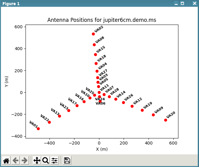
Next, we will use split to split out the following into a new MS.
- 0137+331 (polarization leakage calibrator)
- 1331+305 (3C286 flux density scale and polarization angle calibrator)
- JUPITER* (the asterisk indicates a wildcard and will include all Jupiter fields)
- C-band (6cm): spw='4,5'
split(vis='FLUX99.ms', outputvis='jupiter6cm.demo.ms', field='1331+305,0137+331,JUPITER*', spw='4,5')
At this point, you may wish to run listobs on this new MS. Note, with the new MS the spws will be renumbered starting at 0.
Next use plotants to check the array configuration and select a reference antenna. Here, we will use antenna '11' as a reference since it is located in the middle of the array.
# Figure 1
plotants(vis='jupiter6cm.demo.ms', figfile='jupiter6cm.demo.ant.png')
Note (for uvfits sourced directly from archive only): CASA 5.4 and earlier versions will not plot the antennas properly. This is to be resolved in future CASA versions. If this occurs then a reference antenna can be selected using the listobs task and choosing an antenna located on a pad close to the center of the array (Pads numbers increase with distance from the center of the array, ie. "VLA:_N1" and "EVLA:W2" are pads close to the center of the array, where as, "VLA:_N18" is not).
Data Inspection and Flagging
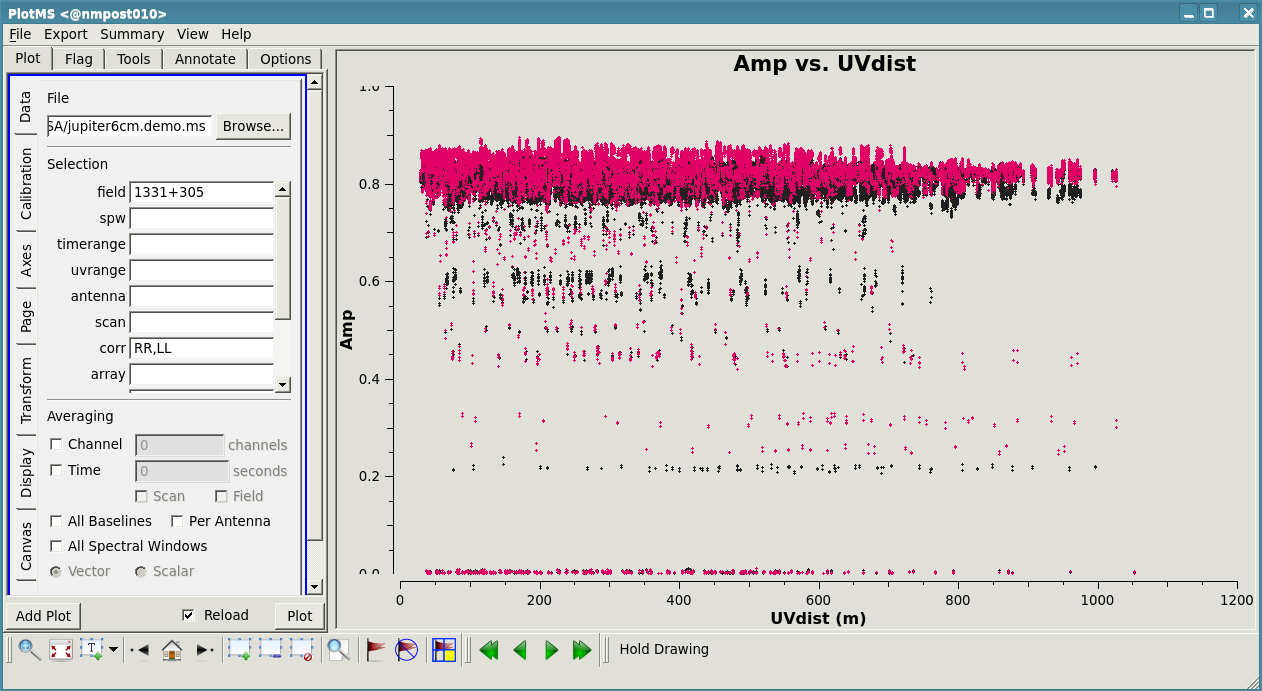
In this section we present two methods of flagging the data:
- Interactive flagging using plotms, which is destructive to the data set and cannot be undone. If a mistake is made, you must start over with a new copy of the data set. Because of the destructive nature of this method, it is generally not recommended.
- Non-interactive flagging using flagdata, which is not destructive to the data set and can be undone (be sure to set flagbackup=True). If a mistake is made, you may undo the flagged data. This is the recommended approach to flagging any data set, new (JVLA) or old (VLA).
For both methods (interactive and non-interactive flagging), we will use plotms to inspect the data.
# Figure 2
plotms(vis='jupiter6cm.demo.ms', selectdata=True, field='1331+305', correlation='RR,LL', xaxis='uvdist', yaxis='amp')
Inspect the following in the data set:
- The primary flux density scale and polarization angle calibrator, 1331+305 (3C286).
- RR,LL and RL,LR correlations separately due to large amplitude differences between them (when all correlations are plotted together, the RL,LR will seem like bad data due to their much lower amplitudes as compared to RR,LL).
- The other two sources we are interested in, the polarization leakage calibrator (0137+331) and the target source (JUPITER).
Interactive Flagging
- Use Mark Regions within the plotms GUI to draw boxes around points to flag, and hit Flag to flag.
Non-Interactive Flagging
- Use plotms to inspect the data set and flagdata to flag the data. While inspecting the data, you may notice that Antenna 9 (ID=8) in spw='1' is often bad. The bad data on Antenna 9 are in the last 4 scans in spw='1' for the 0137+331 calibrator and spw='1' for the target source (JUPITER), as well as in the last scan for all antennas in both spws on the target source. We can flag these points with the following flagdata task executions.
flagdata(vis='jupiter6cm.demo.ms', mode='manual', field='0137+331', spw='1', antenna='9', timerange='42:00:00~48:00:00', flagbackup=True)

flagdata(vis='jupiter6cm.demo.ms', mode='manual', field='JUPITER*', spw='1', antenna='9', timerange='16:26:00~22:20:00', flagbackup=True)

flagdata(vis='jupiter6cm.demo.ms', mode='manual', field='JUPITER*', spw='0,1', timerange='21:40:00~22:20:00', flagbackup=True)
- There are more data points to flag -- keep flagging until you are happy with the results. The following commands will get rid of most bad data. However, depending on how clean the data you want to proceed with, you may still want to inspect them in plotms and flag interactively the remainder of bad data points.
flagdata(vis='jupiter6cm.demo.ms',mode='clip',field='1331+305',correlation='ABS_RR,LL',clipoutside=False,clipminmax=[0,0.75], flagbackup=True)

flagdata(vis='jupiter6cm.demo.ms',mode='clip',field='1331+305',correlation='ABS_RL,LR',clipoutside=False,clipminmax=[0,0.04], flagbackup=True)

flagdata(vis='jupiter6cm.demo.ms',mode='clip',field='0137+331',correlation='ABS_RR,LL',clipoutside=False,clipminmax=[0,0.55], flagbackup=True)

flagdata(vis='jupiter6cm.demo.ms',mode='clip',field='0137+331',correlation='ABS_RL,LR',clipoutside=False,clipminmax=[0,0.01], flagbackup=True)
If you are unfamiliar with flagging in CASA, consult the detailed topical guide Flagging VLA Data.
Calibration
Flux Density Scale
Next we will use setjy to set the absolute flux density scale, only for Stokes I at the moment (the total flux density model).
- Our primary flux calibrator here is 1331+305 (3C286).
- The default model for CASA 5.5+ is 'Perley-Butler 2017'.
setjy(vis='jupiter6cm.demo.ms', field='1331+305', model='3C286_C.im', usescratch=True)
Initial Gain Calibration
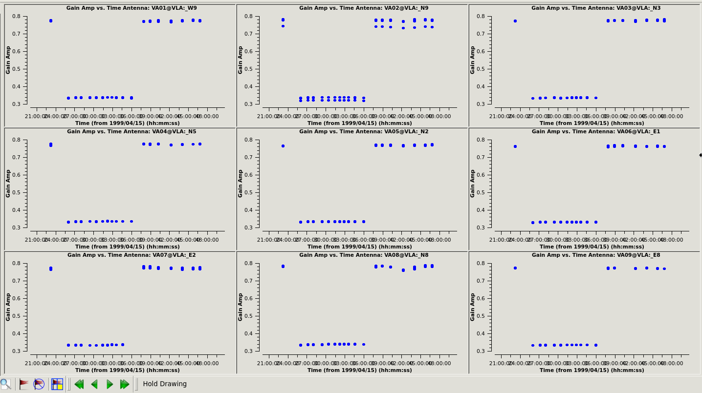
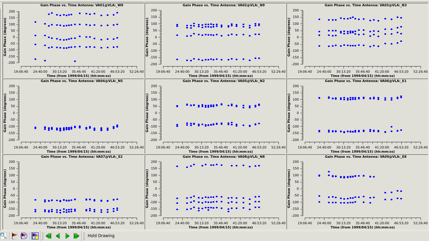
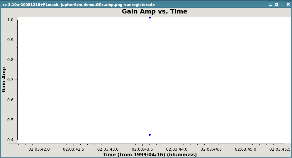
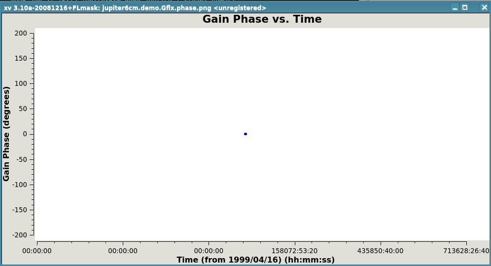
At this stage the data have an overall flux density scaling determined, but full gain solutions aren't there yet. The relevant task is gaincal (analogous to the AIPS task CALIB). Gaincal will produce a separate table with solutions, and we will use appropriate extensions to keep track of the different tables and their corresponding solutions (e.g., gain curve table = .gc).
NOTE: Since we have only two single-channel continuum spw, we do not want to do bandpass calibration nor solve for delays within spws as is currently done with wide bandwidth JVLA data.
First, generate an antenna zenith-angle dependent VLA gain curve calibration table.
gencal(vis='jupiter6cm.demo.ms', caltable='jupiter6cm.demo.gc', caltype='gc')
Now, solve for antenna gains on 1331+305 and 0137+331, using the generated gain curve table (.gc).
gaincal(vis='jupiter6cm.demo.ms', caltable='jupiter6cm.demo.G', field='1331+305,0137+331', spw='', gaintype='G', calmode='ap', solint='inf', combine='', refant='11', minsnr=3, gaintable=['jupiter6cm.demo.gc'], parang=False)

# And check the solutions
# Figure 3:
plotms(vis='jupiter6cm.demo.G', xaxis='time', yaxis='amp', gridrows=3, gridcols=3, iteraxis='antenna')

# Figure 4:
plotms(vis='jupiter6cm.demo.G', xaxis='time', yaxis='phase', plotrange=[-1,-1,-200,200], gridrows=3, gridcols=3, iteraxis='antenna')
If all looks good, bootstrap the flux density scale of the flux calibrator onto the phase calibrators (CASA's fluxscale task is equivalent to GETJY in AIPS). When executing fluxscale, the calibration table with the extension .G is modified and stored as a new table with the extension .Gflx.
myFluxscale = fluxscale(vis='jupiter6cm.demo.ms', caltable='jupiter6cm.demo.G', fluxtable='jupiter6cm.demo.Gflx', reference='1331+305', transfer='0137+331', incremental=True, append=False, display=False)
The output is displayed in the logger as well as stored in the myFluxscale python dictionary.
Beginning fluxscale--(MSSelection version)-------
Generating an incremental caltable
Found reference field(s): 1331+305
Found transfer field(s):  0137+331
Flux density for 0137+331 in SpW=0 (freq=4.8851e+09 Hz) is: 5.29771 +/- 0.00449469 (SNR = 1178.66, N = 54)
Flux density for 0137+331 in SpW=1 (freq=4.8351e+09 Hz) is: 5.34972 +/- 0.00176213 (SNR = 3035.93, N = 54)
Fitted spectrum for 0137+331 with fitorder=1: Flux density = 5.32365 +/- 0 (freq=4.86004 GHz) spidx: a_1 (spectral index) =-0.949536 +/- 0 covariance matrix for the fit:  covar(0,0)=2.07079e-07 covar(0,1)=6.84111e-05 covar(1,0)=6.84111e-05 covar(1,1)=0.0414925
Creating G Jones table from specified parameters.
Generating 'G Cal' corrections.
. . .

Storing result in jupiter6cm.demo.Gflx
Writing solutions to table: jupiter6cm.demo.Gflx
Before proceeding, inspect the flux density calibration and save results to a file.
plotms(vis='jupiter6cm.demo.Gflx', xaxis='time', yaxis='amp', showgui=True, plotfile='jupiter6cm.demo.Gflx.amp.png')

plotms(vis='jupiter6cm.demo.Gflx', xaxis='time', yaxis='phase', plotrange=[-1,-1,-200,200], showgui=True, plotfile='jupiter6cm.demo.Gflx.phase.png')
- Figure 5 (jupiter6cm.demo.Gflx.amp.png) will show two data points: the value at 1.0 is from 3C286 and the value at 0.42 is the complex gain calibrator. The reason 3C286 is 1.0 is because it is used as the reference and the complex gain calibrator is the flux ratio referenced to 3C286, which is assumed 1.0. In this observation, 3C286 was used as the flux density reference.
- Figure 6 (jupiter6cm.demo.Gflx.phase.png) will show two data points at zero (plotted on top of each other). Since we are just scaling amplitudes, we are not expecting the phases to be modified by this calibration table, thus the phases are zero.
Polarization Calibration
Just as in the step of the initial gain calibration, since our old VLA data have single-channel continuum spws, we do not want to solve for KCROSS delays in our polarization calibration. Instead, we directly solve for D and X terms.
Set the Polarization Model
First, set the polarization model for the polarized position-angle calibrator (here 1331+305=3C286 which is also our primary flux calibrator). For polarization properties of your primary polarization calibrator see the Polarimetry section of the VLA Observing Guide.
from math import log
i0=7.3109                                # Stokes I value for spw0 ch0
f0=4.8851                                # Frequency for spw0 ch0 (note that in our data the 'lower' spw is actually higher frequency)
alpha=log(i0/7.35974932)/log(4.8351/f0)  # Values from our setjy() run on Stokes I earlier
c0=0.114                                 # Fractional polarization 11.4% for 5GHz
import numpy as np
d0=33*np.pi/180                          # Polarization angle 33deg in radians

myPolSetjy = setjy(vis='jupiter6cm.demo.ms', field='1331+305', standard='manual', spw='', fluxdensity=[i0,0,0,0], spix=[alpha,0], reffreq=str(f0)+'GHz', polindex=[c0,0], polangle=[d0,0], scalebychan=True, usescratch=True)
The results are displayed in the CASA logger as well as saved in the myPolSetjy python dictionary
#In CASA,
myPolSetjy

#the output below
{'1': {'0': {'fluxd': array([7.3109    , 0.33899165, 0.7613877 , 0.        ])},
  '1': {'fluxd': array([7.26237491, 0.33674164, 0.7563341 , 0.        ])},
  'fieldName': '1331+305'},
 'format': "{field Id: {spw Id: {fluxd: [I,Q,U,V] in Jy}, 'fieldName':field name }}"}
Solve for the Leakage Terms (D terms)
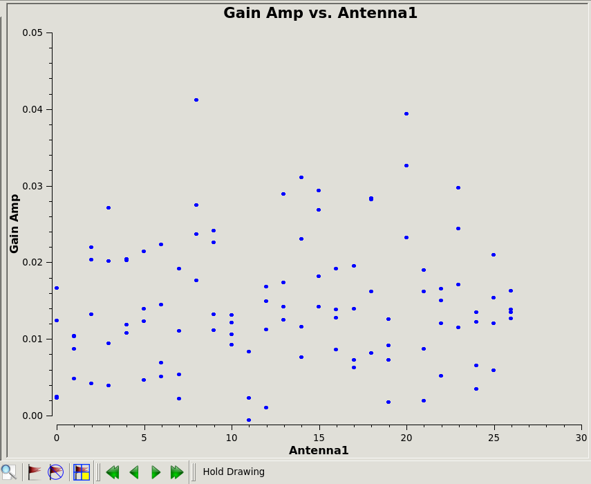
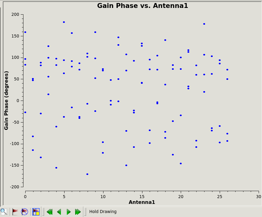
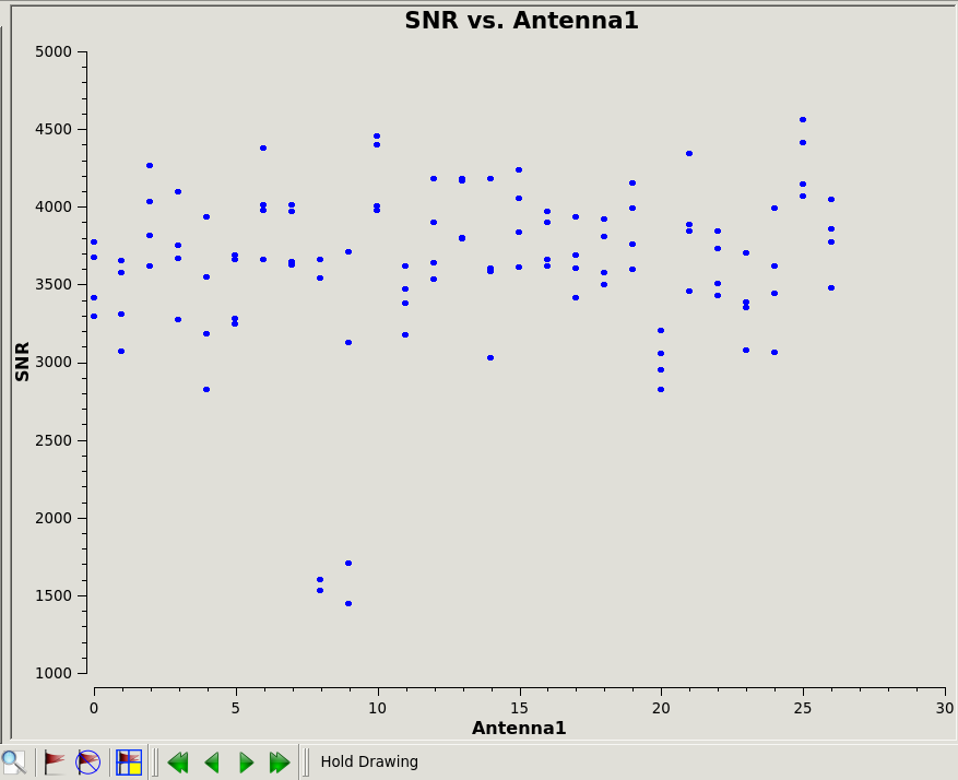
In this step we solve for the instrumental polarization. Solving for polarization leakage on 0137+331, we will assume our calibrator has unknown polarization.
- if good parallactic coverage, poltype='D+QU'
- otherwise, poltype='D'
Consult polcal for more information on options.
polcal(vis='jupiter6cm.demo.ms', caltable='jupiter6cm.demo.D', field='0137+331', spw='', refant='11', poltype='D+QU', solint='inf', combine='scan',minsnr=3, gaintable=['jupiter6cm.demo.gc', 'jupiter6cm.demo.G'], gainfield=['','0137+331',''])
Check the solutions
# Figure 7:
plotms(vis='jupiter6cm.demo.D', xaxis='antenna1', yaxis='amp', showgui=True, plotfile='jupiter6cm.demo.D.amp.png')

# Figure 8:
plotms(vis='jupiter6cm.demo.D', xaxis='antenna1', yaxis='phase', plotrange=[-1,-1,-200,200], showgui=True, plotfile='jupiter6cm.demo.D.phase.png')

# Figure 9:
plotms(vis='jupiter6cm.demo.D', xaxis='antenna1', yaxis='snr', showgui=True, plotfile='jupiter6cm.demo.D.snr.png')
Solve for the R-L Polarization angle (X term)
The total polarization is now correct (since we just calibrated the instrumental polarization, i.e., D terms). Now the R-L phase needs to be calibrated to obtain an accurate polarization position angle.
polcal(vis='jupiter6cm.demo.ms', caltable='jupiter6cm.demo.X', field='1331+305', spw='', refant='11', poltype='Xf', solint='inf', combine='scan',minsnr=3, gaintable=['jupiter6cm.demo.gc', 'jupiter6cm.demo.G', 'jupiter6cm.demo.D'], gainfield=['','1331+305','',''])
Check the solutions in the CASA logger window
The following calibration term is arranged for solve:
.   Xf Jones: table=jupiter6cm.demo.X append=false solint=inf,none refantmode='flex' refant='none' minsnr=3 apmode=AP solnorm=false
For solint = inf, found 2 solution intervals.
Mean CROSS-HAND PHASE solution for 1331+305 (spw = 0) = 28.7301 deg.
Mean CROSS-HAND PHASE solution for 1331+305 (spw = 1) = -59.9972 deg.
  Found good Xf Jones solutions in 2 solution intervals.
NOTE: If you are using CASA 4.7 or earlier, you may want to use poltype='X' in X-term calculations (Mueller matrices). For CASA 5.0 and later this option will not work (the relevant CASA documentation is being updated), and hence you need to use poltype='Xf' (Jones matrices). Although 'Xf' should be used predominantly for large bandwidths, which clearly is not the case here, it can also be used for the single channel old VLA data as long as you make sure the interp parameter is set to default (which should be nearest).
Apply the Calibration
Now that we have derived all the calibration solutions and saved them in the tables of multiple extensions, we need to apply them to the actual data. The applycal task commands will apply the solution tables to the DATA column and write a new column CORRECTED_DATA as it is standard for CASA. Important: make sure you set parang=True.
applycal(vis='jupiter6cm.demo.ms', field='1331+305', spw='', selectdata=False, gaintable=['jupiter6cm.demo.gc', 'jupiter6cm.demo.G', 'jupiter6cm.demo.D','jupiter6cm.demo.X'], gainfield=['','1331+305'], calwt=[False], parang=True)

applycal(vis='jupiter6cm.demo.ms', field='0137+331', spw='', selectdata=False, gaintable=['jupiter6cm.demo.gc', 'jupiter6cm.demo.G', 'jupiter6cm.demo.Gflx','jupiter6cm.demo.D','jupiter6cm.demo.X'], gainfield=['','0137+331','0137+331'], calwt=[False], parang=True)

applycal(vis='jupiter6cm.demo.ms', field='JUPITER*', spw='', selectdata=False, gaintable=['jupiter6cm.demo.gc', 'jupiter6cm.demo.G', 'jupiter6cm.demo.Gflx','jupiter6cm.demo.D','jupiter6cm.demo.X'], gainfield=['','0137+331','0137+331'], calwt=[False], parang=True)
Next, we will split the corrected (i.e., calibrated) Jupiter target data from the MS we started with and write it to a new single-source MS.
split(vis='jupiter6cm.demo.ms', outputvis='jupiter6cm.demo.JUPITER.split.ms', field='JUPITER*', datacolumn='corrected')
You can use the plotms task to look at the split calibrated data.
Initial Imaging (Stokes I)
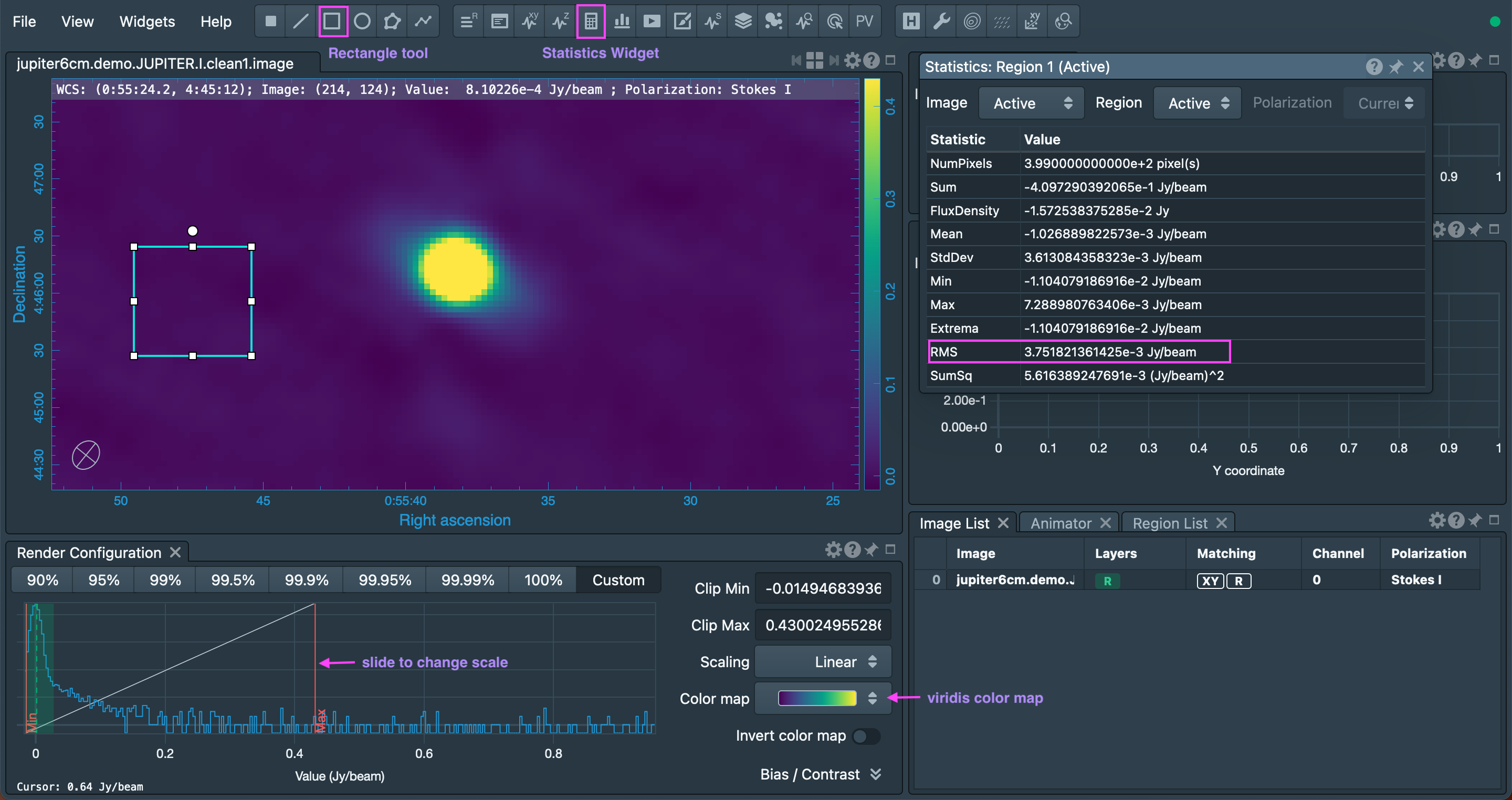
Next we will image and clean the Jupiter data. In this step we will self-calibrate, therefore in the initial imaging we will not clean too deeply and we will save the model in the MS data (with the use of parameter savemodel in tclean).
Since we set mask="" in tclean, the interactive GUI will not allow you to do the deconvolution before you draw the mask on at least one plane. When drawing a mask, be sure to select All Channels and All Polarizations each time you run tclean.
tclean(vis='jupiter6cm.demo.JUPITER.split.ms', stokes='I', field='', spw='', imagename='jupiter6cm.demo.JUPITER.I.clean1', robust = 0.0, imsize=[288], cell=['3arcsec'], specmode='mfs', deconvolver='hogbom', weighting='briggs', threshold='0.1mJy', mask='', niter=500, interactive=True, cycleniter=100, savemodel='modelcolumn', pblimit=-0.2)
Next we will use CARTA to inspect the quality of the cleaned image and we can use the Statistics Widget to tell us the rms. Once you have loaded CARTA using the instructions from the link, proceed with the following steps:
- Load the cleaned image, jupiter6cm.demo.JUPITER.I.clean1.image
- If you would like your images to use the same Color map as this guide, select viridis (at the bottom of the list).
- Hover your mouse over the image to reveal the zoom icons near the bottom of the image. Zoom in/out as much as you wish.
- Near the top, select the Rectangle tool and draw a box in the blank space next to Jupiter.
- Near the top, select the Statistics Widget (tiny calculator icon). Here you will see the rms of the sky around Jupiter. These numbers will change as you move the box around the blank sky.
For an annotated visual example, refer to Figure 10. (Note, this session of CARTA is using the Dark mode theme found under View.)
In this initial imaging, the deconvolution will stop with the iteration limit since we set it fairly low. We 'cleaned' approximately 4.3 Jy in this initial imaging step, and reached rms of about 3.64 mJy/bm.
Self-Calibration
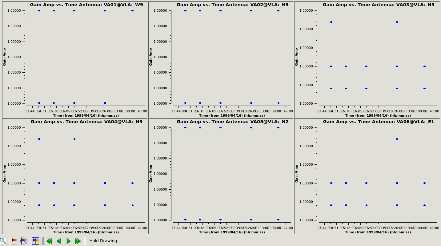
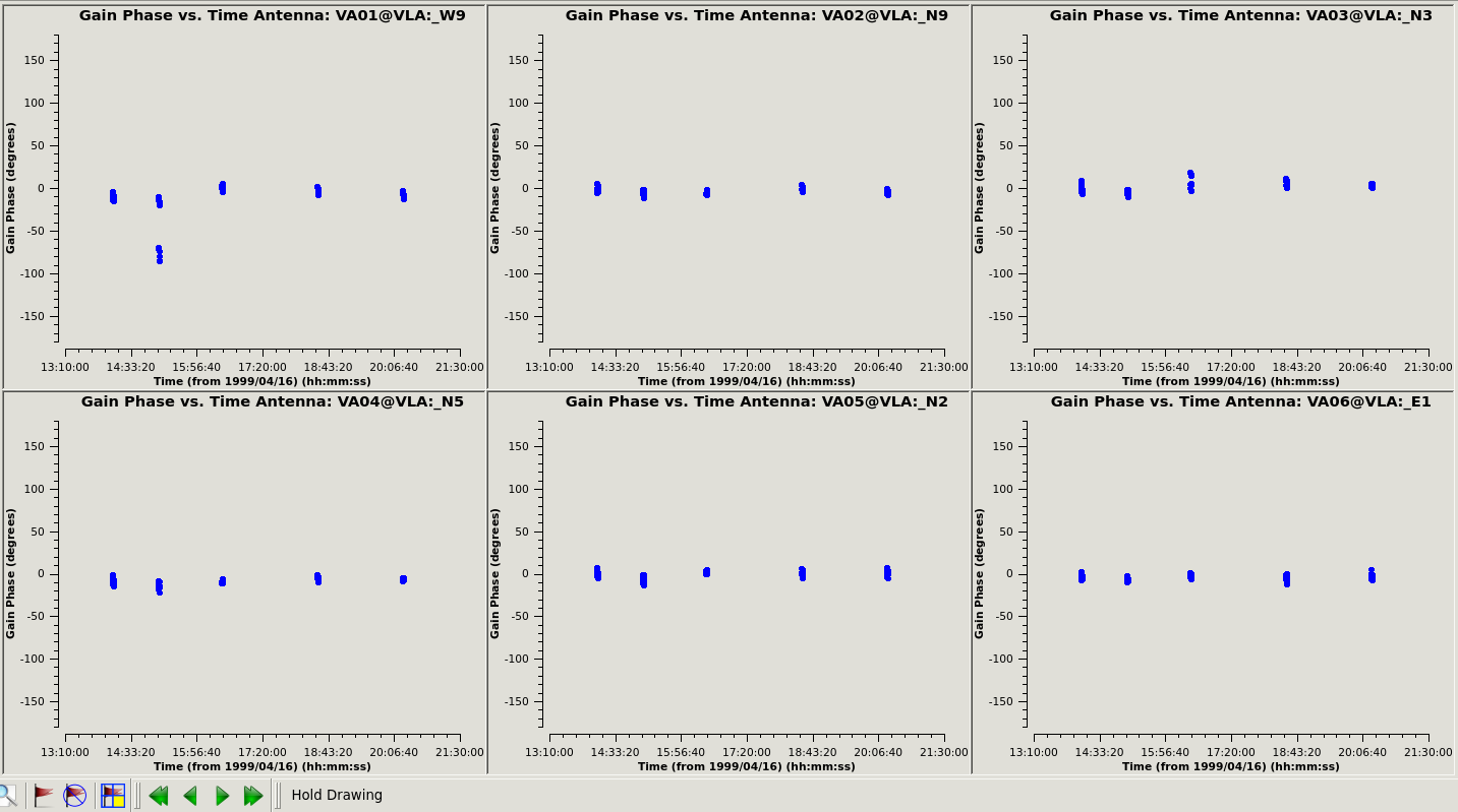

In the self-calibration step we run gaincal that will make use of the newly created MODEL column in our MS file.
gaincal(vis='jupiter6cm.demo.JUPITER.split.ms', caltable='jupiter6cm.demo.JUPITER.split.selfcal1', field='', spw='', gaintype='G', calmode='p', solint='30s', combine='', refant='11', parang=False, append=False, selectdata=False)
Inspect the solutions using plotms.
# Figure 11:
plotms(vis='jupiter6cm.demo.JUPITER.split.selfcal1',xaxis='time',yaxis='amp',gridrows=2, gridcols=3, iteraxis='antenna')

# Figure 12:
plotms(vis='jupiter6cm.demo.JUPITER.split.selfcal1',xaxis='time',yaxis='phase', gridrows=2, gridcols=3 ,iteraxis='antenna',plotrange=[-1,-1,-180,180])
Next, use applycal to apply the calibration to the DATA (creating a CORRECTED column in the MS).
applycal(vis='jupiter6cm.demo.JUPITER.split.ms', field='', spw='', selectdata=False, gaintable=['jupiter6cm.demo.JUPITER.split.selfcal1'], gainfield=[''], interp=['nearest'],calwt=[False], applymode='calflag')
Now, use tclean to image the self-calibrated data.
tclean(vis='jupiter6cm.demo.JUPITER.split.ms', stokes='I', field='', spw='', imagename='jupiter6cm.demo.JUPITER.I.clean2', robust= 0.0, imsize=[288], cell=['3arcsec'], specmode='mfs', deconvolver='hogbom', weighting='briggs', threshold='0.05mJy', mask='', niter=10000, interactive=True, cycleniter=100, pblimit=-0.2)
Check the image statistics using CARTA. See Figure 13 for details.
- Open both images: jupiter6cm.demo.JUPITER.I.clean1.image and jupiter6cm.demo.JUPITER.I.clean2.image. (Note, only one image can be opened at a time. After you have opened one, you will then need to select File -> Append Image to open another image.)
- In the lower right under Image List, select XY and R (under Matching) for both images. This will allow you to manipulate the images simultaneously.
- Hover your mouse over one of the images to reveal the zoom icons. These will allow you to zoom in/out of the image.
- Near the top, select the Ellipse tool (circle icon) and draw an ellipse around Jupiter for one of the images. Since you selected XY and R for both images, an ellipse drawn on one image will be automatically created on the other image.
- Near the top, select the Statistics Widget (tiny calculator). A small window will pop-up with the statistics of the active image (the last selected image). You may change information shown for an image by either selecting the other image or by selecting the image file name in the Image selector menu located on the Statistics Widget window.
After one cycle of self-calibration with tclean we reached an rms of about 1.10 mJy/bm (in the blank sky). However, keep in mind that the rms values may differ for you since they will depend on how deeply you cleaned and how good a mask you applied. Note, after self-cal the flux of the target should be about the same or higher than before self-cal. If the flux is lower, then something went wrong in the gaincal step for self-cal.
Full Stokes Imaging
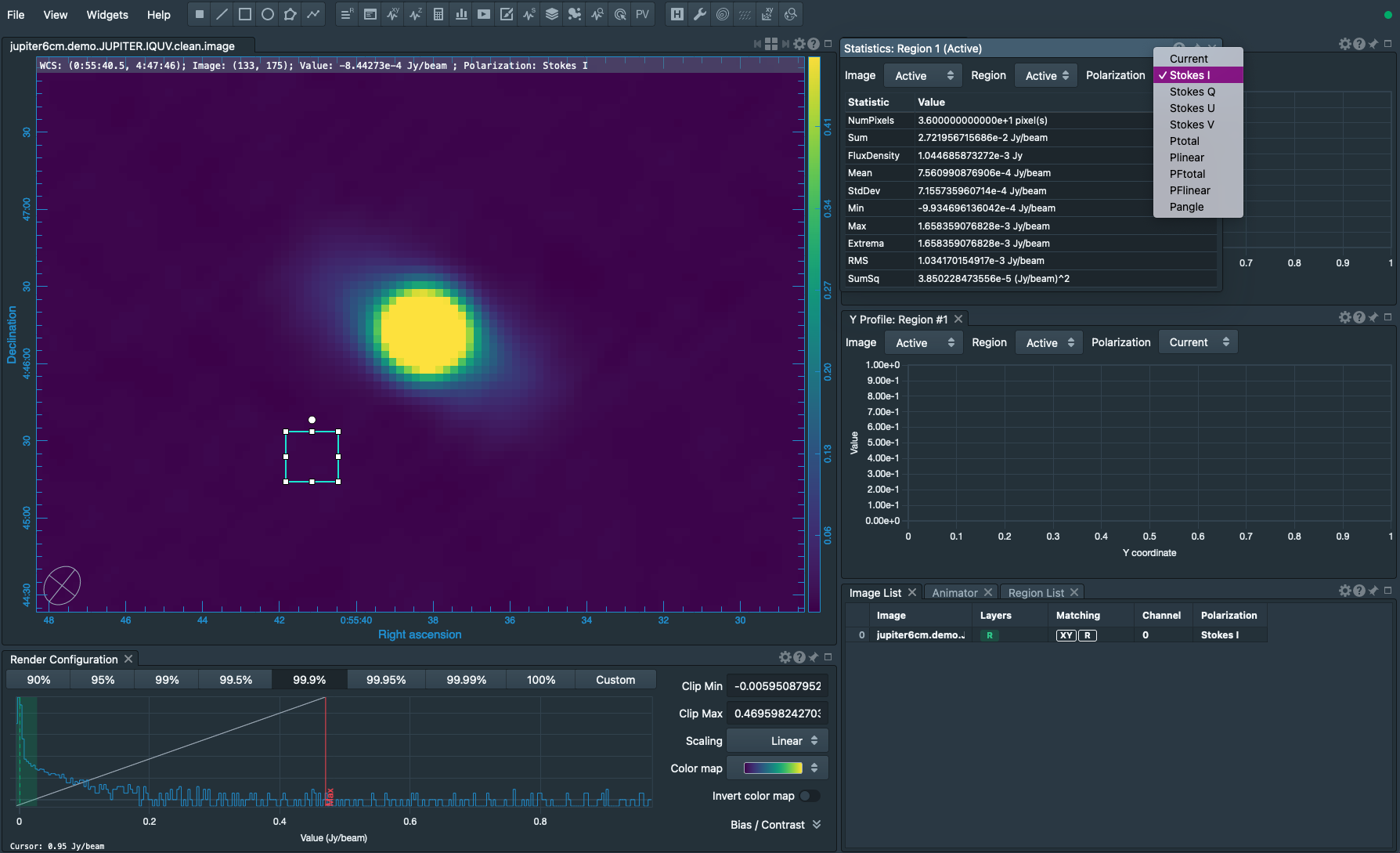
At this stage we will perform full Stokes imaging using tclean to create an image of each Stokes parameter that we will later use to create polarized intensity and angle images.
tclean(vis='jupiter6cm.demo.JUPITER.split.ms', stokes='IQUV', field='', spw='', imagename='jupiter6cm.demo.JUPITER.IQUV.clean', robust= 0.0, imsize=[288], cell=['3arcsec'], specmode='mfs', deconvolver='clarkstokes', weighting='briggs', threshold='0.05mJy', mask='', niter=10000, interactive=True, cycleniter=100, pblimit=-0.2)
Inspect the quality of the cleaned image in CARTA (see Figure 14).
- Open jupiter6cm.demo.JUPITER.IQUV.clean.image,
- Create a box in a blank part of the sky next to Jupiter,
- Select the Statistics Widget, and select the Stokes parameter in the Polarization drop-down menu located in the statistics window.
Depending on how deeply you cleaned, you may reach rms values of about:
- (I) 1.1 mJy/bm
- (Q) 0.62 mJy/bm
- (U) 0.90 mJy/bm
- (V) 0.16 mJy/bm
Polarization Intensity and Position Angle Images
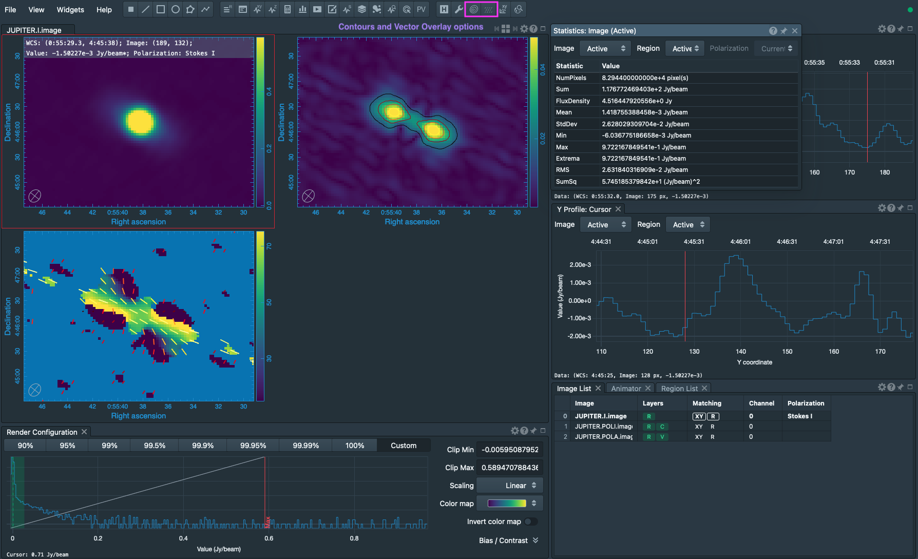
Next, we will save each Stokes plane as separate images. We can use either the imsubimage or immath tasks to do so.
Run the imsubimage task:
imsubimage(imagename='jupiter6cm.demo.JUPITER.IQUV.clean.image',outfile='JUPITER.I.image',stokes='I')

imsubimage(imagename='jupiter6cm.demo.JUPITER.IQUV.clean.image',outfile='JUPITER.Q.image',stokes='Q')

imsubimage(imagename='jupiter6cm.demo.JUPITER.IQUV.clean.image',outfile='JUPITER.U.image',stokes='U')
Or run the immath task:
immath(imagename='jupiter6cm.demo.JUPITER.IQUV.clean.image', mode='evalexpr', stokes='I', expr='IM0', outfile='JUPITER.I.image')

immath(imagename='jupiter6cm.demo.JUPITER.IQUV.clean.image', mode='evalexpr', stokes='Q', expr='IM0', outfile='JUPITER.Q.image')

immath(imagename='jupiter6cm.demo.JUPITER.IQUV.clean.image', mode='evalexpr', stokes='U', expr='IM0', outfile='JUPITER.U.image')
Finally, we want to create the polarization intensity (POLI) and position angle (POLA) images using immath.
immath(imagename=['JUPITER.Q.image','JUPITER.U.image'], mode='poli', outfile='JUPITER.POLI.image')
We will now use the polithresh parameter when creating the polarization angle image to get rid of the noise. First check the statistic in the POLI image, and then use it as a threshold while creating the POLA image (in the example below equal to 4 sigma).
immath(imagename=['JUPITER.Q.image','JUPITER.U.image'], mode='pola', outfile='JUPITER.POLA.image',polithresh='4.5mJy/beam')
Again, check the statistics of these final images with CARTA.
See Figure 15 to view Jupiter, POLI, and POLA images. Note, CARTA cannot yet overlay multiple images. However, it can overlay contours and vectors.
That concludes this tutorial.
For the tutorial on how to perform analysis, display, and manipulation of the polarization images, consult the VLA Continuum Tutorial 3C391.
Last checked on CASA Version 6.4.1