Pipeline: Frequent VLA problems: Difference between revisions
| (140 intermediate revisions by 6 users not shown) | |||
| Line 8: | Line 8: | ||
== Radio Frequency Interference == | == Radio Frequency Interference == | ||
By far the biggest problem is radio frequency interference (RFI). RFI is produced by internal and external sources, can be terrestrial or from satellites that operate at or spill into the observed frequency. For the VLA, please find more information on the [https://science.nrao.edu/facilities/vla/docs/manuals/obsguide/rfi Radio Frequency Interference] webpage. Although weak RFI may only slightly raise the noise of an image, stronger RFI will produce artifacts that may render the data unusable. An example for strong RFI is shown below. Flagging procedures are outlined in the [https://casaguides.nrao.edu/index.php/VLA_CASA_Flagging VLA topical CASA guide on flagging]. | By far the biggest problem is radio frequency interference (RFI). RFI is produced by internal and external sources, can be terrestrial or from satellites that operate at or spill into the observed frequency. For the VLA, please find more information on the [https://science.nrao.edu/facilities/vla/docs/manuals/obsguide/rfi Radio Frequency Interference] webpage. Although weak RFI may only slightly raise the noise of an image with little influence on the calibration tables, stronger RFI will produce artifacts that may render the data (target and calibrators) unusable, if not adequately flagged. An example for strong RFI is shown below. Flagging procedures are outlined in the [https://casaguides.nrao.edu/index.php/VLA_CASA_Flagging VLA topical CASA guide on flagging]. | ||
{| | {| | ||
|[[Image:CASA5.4.0-FLAG-Plotms-amp-time.png|400px|thumb|left|Example for RFI in an observation.]] | |[[Image:CASA5.4.0-FLAG-Plotms-amp-time.png|400px|thumb|left|Figure 1. Example for RFI in an observation.]] | ||
|} | |} | ||
It is important that all data are free of RFI. | |||
<pre style="white-space: pre-wrap; background-color: #E0FFFF;"> | <pre style="white-space: pre-wrap; background-color: #E0FFFF;"> | ||
FIX: Weak, | FIX: Weak, intermittent RFI will increase the noise and be down-weighted in the imaging in the hifv_statwt task. Strong RFI needs to be flagged and only clean data should be calibrated and imaged. Flagging can be manual or automatic. | ||
</pre> | </pre> | ||
== Pointing == | == Pointing == | ||
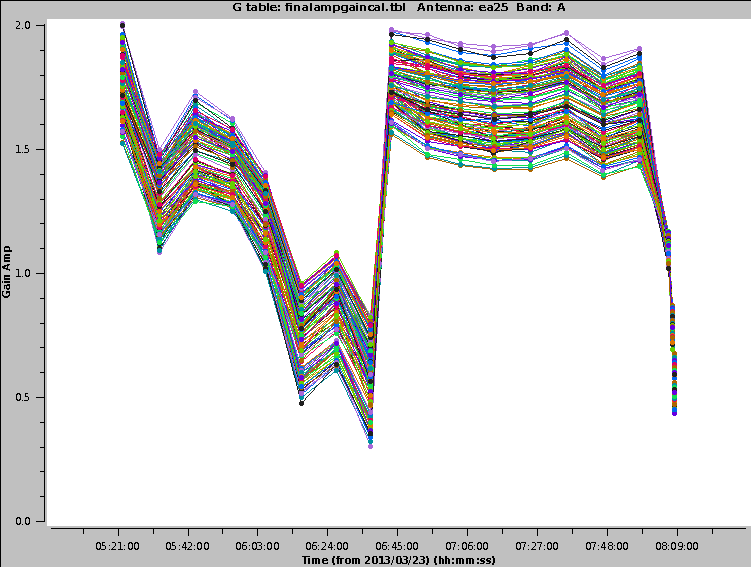
At higher frequencies the VLA requires regular pointing calibrations. Each pointing run will reposition the antennas to be centered on a strong source with known position. If the pointing solution fails, the amplitude of the source will drop. A typical graph looks like the one shown below. The pointing solution for the first half of the run failed, which results in the source drifting away from the center of the primary beam. After a pointing update in the middle of the run, the antenna is positioned properly again (the very last data points are actually a different source, hence the drop at the edge). | At higher frequencies the VLA requires regular pointing calibrations. Each pointing run will reposition the antennas to be centered on a strong source with known position. If the pointing solution fails, the amplitude of the source will drop or drift away from the center of the antenna with the highest gain. A typical graph looks like the one shown below. The pointing solution for the first half of the run failed, which results in the source drifting away from the center of the primary beam. After a pointing update in the middle of the run, the antenna is positioned properly again (the very last data points are actually a different source, hence the drop at the edge). | ||
{| | {| | ||
|[[Image:VLApipe-gains-ea25-CASA6.2.1.png|400px|thumb|left|Example of a gain table with a failed pointing solution in the first half of the observation]] | |[[Image:VLApipe-gains-ea25-CASA6.2.1.png|400px|thumb|left|Figure 2a. Example of a gain table with a failed pointing solution in the first half of the observation]] | ||
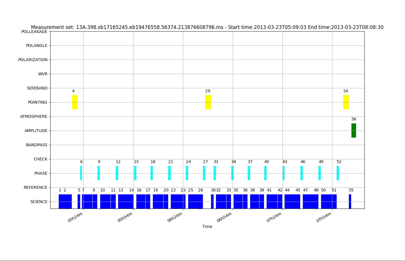
|[[Image:IntentvsTime.png|400px|thumb|left|Figure 2b. Plot showing the scan intents vs time for the same observation.]] | |||
|} | |} | ||
<pre style="white-space: pre-wrap; background-color: #E0FFFF;"> | <pre style="white-space: pre-wrap; background-color: #E0FFFF;"> | ||
FIX: If the pointing is only off by a small amount, the gain calibration will take care of it. If it is off by a large amount, the data for this period and antenna needs to be flagged. | FIX: If the pointing is only off by a small amount, the gain calibration will take care of it. If it is off by a large amount, the data for this period and antenna needs to be flagged. | ||
</pre> | |||
== Phase Jumps == | |||
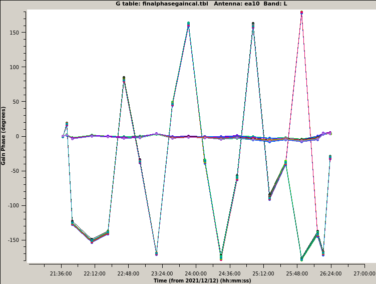
Various hardware failures can cause the phase for a given antenna to be unstable in time, often with sudden, large changes in phase over time. Depending on where the problem is, this may affect just a portion of the data or up to all data on a given antenna. In the example below, only one baseband's data is affected (large changes at each data point) while the other baseband remains near zero and is not affected. This plot, from the pipeline's Final phase gain cal section found in the 'hifv_finalcals' stage, shows the final phase solutions found for each calibrator (using the long solution interval). | |||
{| | |||
|[[Image:phasejumps1.png|400px|thumb|left|Figure 3. Example for phase jumps in an observation.]] | |||
|} | |||
Typical phase variations for low frequency data are a few degrees. For high frequencies tens of degrees can occur; the cycle time between the phase calibrator and the target needs to be reduced to adequately track and interpolate the phase variations as a function of time. If the phases vary more than 360 degrees between two phase calibrator scans, then the data are completely decorrelated and cannot be calibrated anymore (even changes larger than 180deg leave the interpolation pretty much undefined). | |||
<pre style="white-space: pre-wrap; background-color: #E0FFFF;"> | |||
FIX: If there are phase jumps, usually the data for the affected time range needs to be flagged for the antenna(s). | |||
</pre> | </pre> | ||
| Line 33: | Line 50: | ||
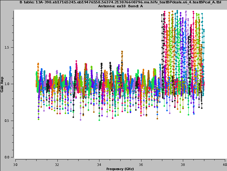
The digital transmission system (''DTS'') of each VLA antenna includes a formatting stage to convert the electronic to | The digital transmission system (''DTS'') of each VLA antenna includes a formatting stage to convert the electronic signal to optical before it is injected on the optical fiber link. On the correlator end the signal will be deformatted back to an electronic signal. Occasionally the timing on the deformatter can be misaligned, which results in very strong amplitude or phase slopes as a function of frequency. When this occurs, the data are corrupt and the entire affected baseband per polarization of an antenna need to be flagged. Frequently the error shows up similar to an ''abs(sin)'' or a 'bouncing' signal across a baseband for one polarization or, in other terms, various numbers of 'V' shapes in the data, usually in the middle of a baseband. | ||
{| | {| | ||
|[[Image:VLApipe-step6-BPgain-ea18-CASA6.2.1.png|400px|thumb|left| | |[[Image:VLApipe-step6-BPgain-ea18-CASA6.2.1.png|400px|thumb|left|Figure 4a. DTS issue in one baseband]] | ||
|[[Image:VLApipe-baddefromatterexampleBP.png|400px|thumb|left| | |[[Image:VLApipe-baddefromatterexampleBP.png|400px|thumb|left|Figure 4b. An example of a bad deformatter from a different dataset.]] | ||
|} | |||
{| | |||
|[[Image:badDTS1.png|400px|thumb|left|Figure 4c. Another instance of a DTS issue]] | |||
|[[Image:badDTS2.png|400px|thumb|left|Figure 4d. DTS example that is more continuous since the gain and amplitudes are not normalized]] | |||
|} | |} | ||
Sometimes, however, the pipeline erroneously detects a DTS issue, when the data were in fact only affected by RFI in a few spws. If that happens it is better to flag the data manually, which preserves the rest of the baseband. | |||
<pre style="white-space: pre-wrap; background-color: #E0FFFF;"> | <pre style="white-space: pre-wrap; background-color: #E0FFFF;"> | ||
FIX: The data | FIX: The data for this baseband, antenna and polarization need to be flagged. | ||
</pre> | </pre> | ||
== Correlator Zeros == | == Correlator Zeros == | ||
Under some circumstances, the WIDAR correlator writes exact zeros. The pipeline will usually flag them automatically. If not, they can be removed with CASA | Under some circumstances, the WIDAR correlator writes exact zeros. The pipeline will usually flag them automatically. If not, they can be removed with CASA's [https://casadocs.readthedocs.io/en/v6.2.1/api/tt/casatasks.flagging.flagdata.html flagdata] task, using the option ''mode='clip' '' with ''clipzeros=True'' or flag the zeros by hand. | ||
{| | |||
|[[Image:FlaggedDataSummary.png|400px|thumb|left|Figure 5. If using the pipeline one can find the above table in the hifv_flagdata task. Here the percentage of data flagged due to correlator zeros is represented by the "Clipping" column.]] | |||
|} | |||
The percentage is calculated based on channels. Spectral line spws are therefore more susceptible to a high reported number of zeros. | |||
<pre style="white-space: pre-wrap; background-color: #E0FFFF;"> | <pre style="white-space: pre-wrap; background-color: #E0FFFF;"> | ||
| Line 54: | Line 82: | ||
== Baseband and Subband Edges == | == Baseband and Subband Edges == | ||
If spw roll-off frequency edges are very steep, they can degrade gain and phase solutions. Frequently this is not a big problem, but if the gain for the edge channels is close to zero, a division by the bandpass for these channels can get extremely noisy. | If spw roll-off frequency edges are very steep, they can degrade gain and phase solutions. Frequently this is not a big problem, but if the gain for the edge channels is close to zero, a division by the bandpass for these channels can get extremely noisy. This is particularly true for baseband edges. The ''edgespw'', ''fracspw'', and ''baseband'' parameters in ''hifv_flagdata'' can be adjusted to flag different percentages of the edges (see also [http://go.nrao.edu/vla-pipe VLA pipeline] pages). The edges can also be flagged with the CASA task [https://casadocs.readthedocs.io/en/v6.2.1/api/tt/casatasks.flagging.flagdata.html flagdata], or by hand. | ||
<pre style="white-space: pre-wrap; background-color: #E0FFFF;"> | <pre style="white-space: pre-wrap; background-color: #E0FFFF;"> | ||
| Line 62: | Line 89: | ||
</pre> | </pre> | ||
== | == Resolved Calibrators == | ||
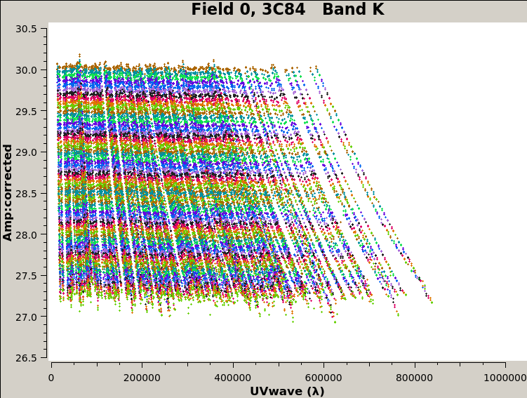
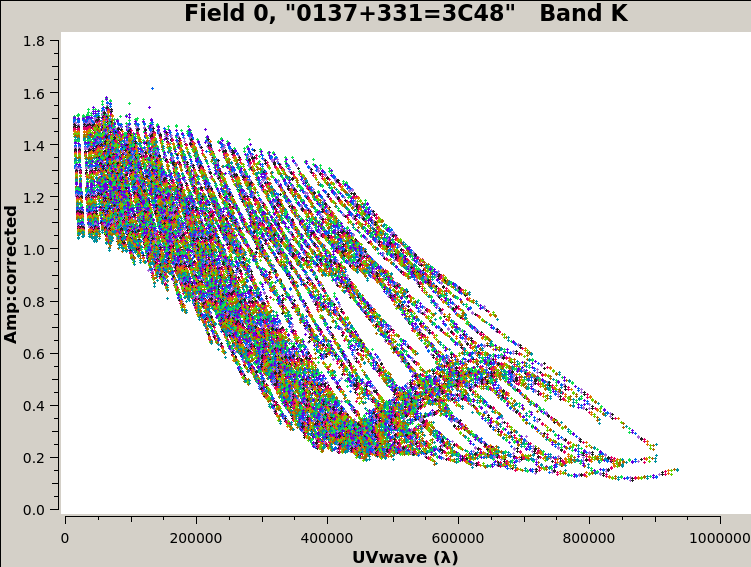
Some calibrator sources are not perfect point sources. For the VLA standard flux calibrator sources, models are provided within CASA, which solves the problem for these. Resolved phase calibrators, however, will produce an more or less incorrect gaintable. In some cases, CASA's gaincal can even fail completely and set all fluxes to 1Jy. To work with resolved gain/phase calibrators, either provide a model, or, at least, restrict the uv-range to the unresolved portion during the solve. Plotting the amplitude against uv distance (uvwave) should clearly show the flat part that can be used, and the non-flat parts that should be omitted. Try to make sure though, that there are at least some baselines for every antenna available for the solve. Figures 6a and 6b show, respectively, the visibility data for an unresolved and a resolved calibrator. | |||
{| | |||
|[[Image:3C84_AmpvsUVwave.png|400px|thumb|left|Fig. 6a. Plot showing the point-like nature of 3C84 during a K-band, B-config observation. Point-like sources will appear as horizontal lines in such plots.]] | |||
|[[Image:3C48_AmpvsUVwave.png|400px|thumb|left|Fig. 6b. Plot showing resolved structure in 3C48 during a K-band, B-config observation. However, due to being one of the VLA's standard flux calibrators, this structure will be accounted for when setting the model for this source.]] | |||
|} | |||
A solution is to use the flux.csv table. It is usually generated for ALMA in a pipeline run, but can be created before a VLA run. The uv-ranges listed there will be used in the processing. The format is like: | |||
ms,field,spw,I,Q,U,V,spix,uvmin,uvmax,comment | |||
and an example entry would be: | |||
MY.ms,0,2,1.0,0.0,0.0,0.0,0.0,21000.0,110000.0,"3C48" | |||
for a uvrange of 21000-110000 lambda. | |||
Above, ms is the MS name, field and spw are the IDs (not names, the ID will only be known once the data is in MS format and after executing listobs), I, Q, U, V are the Stokes flux densities in Jy (note that entries for the VLA will be ignored here, so a nominal I=1.0Jy will be ok), uvmin and uvmax are the uv ranges in units of lambda. Only one spw (the first) is used per field, other entries will be ignored. This means a single line entry such as the one above will apply to all spws for the given field. When using a uvrange, note that both a uvmin and uvmax must be specified: if one wants to specify only a uvmax, we suggest setting a uvmin of 0.01. If uvmax is provided as 0.0 lambda, then this creates an inequality and uvmax is unbounded. | |||
If you have multi-band data, you may have to split the data per band first, then run each band through their own pipeline to make use of flux.csv. | |||
<pre style="white-space: pre-wrap; background-color: #E0FFFF;"> | <pre style="white-space: pre-wrap; background-color: #E0FFFF;"> | ||
FIX: Restrict the uv-range for the calculations of the calibration tables. | FIX: Restrict the uv-range for the calculations of the calibration tables. The flux.csv table can be used. | ||
</pre> | </pre> | ||
| Line 84: | Line 123: | ||
== Non-ideal reference antenna == | == Non-ideal reference antenna == | ||
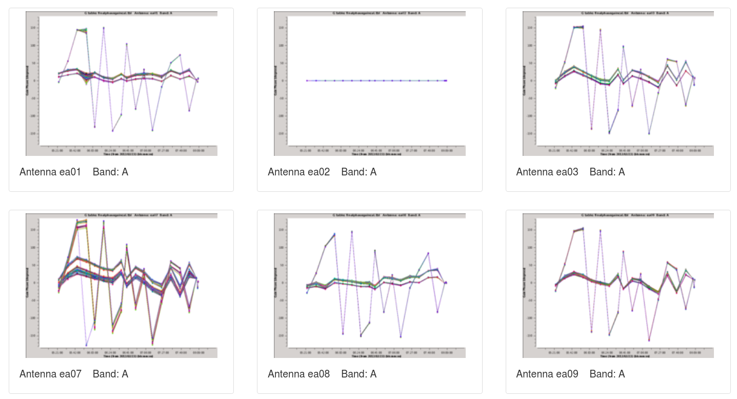
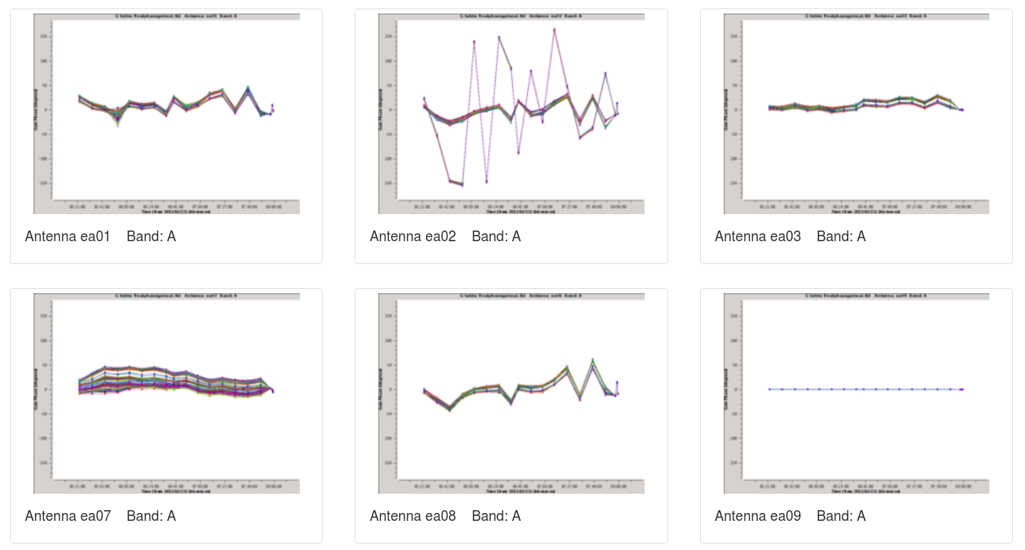
Sometimes | Sometimes if the reference antenna has some issue, like RFI or extreme flagging, it is advisable to switch to a different reference antenna. The example below shows that one spw has extreme phase jumps for all antennas when ea02 was chosen as a reference antenna (Fig. 7a). This indicates that the phase jumps are likely not present on all antennas, but that phase instabilities on ea02 itself are reflected on all other antennas. Indeed, when ea09 was chosen as a reference antenna, as shown in Fig. 7b, then the instability is shown only in ea02 and all other antennas are well-behaved. | ||
Delays are also a quantity that are relative to a chosen reference antenna. If the delays for all antennas show similarly high delays, then it is likely that the reference antenna has the high delays and not all other antennas. Chosing a different reference antenna would quickly reveal if this is the case. | |||
Use the 'refantignore' keyword to disallow the use of this antenna as a reference (in the example one should ignore ea02 as a possible reference antenna). The [https://science.nrao.edu/facilities/vla/data-processing/pipeline Pipeline Page] provides details on the usage of this keyword. | |||
{| | |||
|[[Image:Bad_refant.png|400px|thumb|left|Fig. 7a. Plots of phase solutions vs time showing that all antennas have inherited ea02's phase issue when it is used as the reference antenna.]] | |||
|[[Image:Good_refant.png|400px|thumb|left|Fig 7b. Plots of phase solutions vs time showing ea02 has a phase issue. Here ea09 is used as the reference antenna.]] | |||
|} | |||
<pre style="white-space: pre-wrap; background-color: #E0FFFF;"> | <pre style="white-space: pre-wrap; background-color: #E0FFFF;"> | ||
FIX: Use 'refantignore' to remove | FIX: Use 'refantignore' to remove a problematic antenna from the list of possible reference antennas. | ||
</pre> | </pre> | ||
== Extreme Solution Intervals == | == Extreme Solution Intervals == | ||
In the hifv_solint stage, the short solution interval is computed as the longest individual single integration (dump) of a visibility. The long solution interval is the longest scan on the gain/phase calibrator. If those values seem unreasonable, then the data should be inspected and flagged. Sometimes, the observations are set up with a long phase calibrator scan at the beginning, to allow for longer slews to the source. This can result in excessive long solints, and some flagging may be advised on this scan. | |||
After flagging, the pipeline should then be re-run to determine new solution intervals. | |||
{| | |||
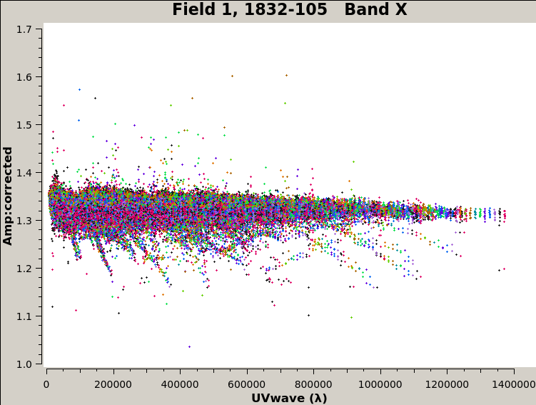
|[[Image:LongSolint.png|400px|thumb|left|Fig. 8a. Corrected Amplitude vs UVwave for a complex gain calibrator taken in X-band, A-config. The observation used a long initial complex gain calibration scan to account for slew time. The amount of time to slew to the source was shorter than expected and resulted in the pipeline using a long solution interval of ~160s. Decorrelation is evident from the low amplitude streaks.]] | |||
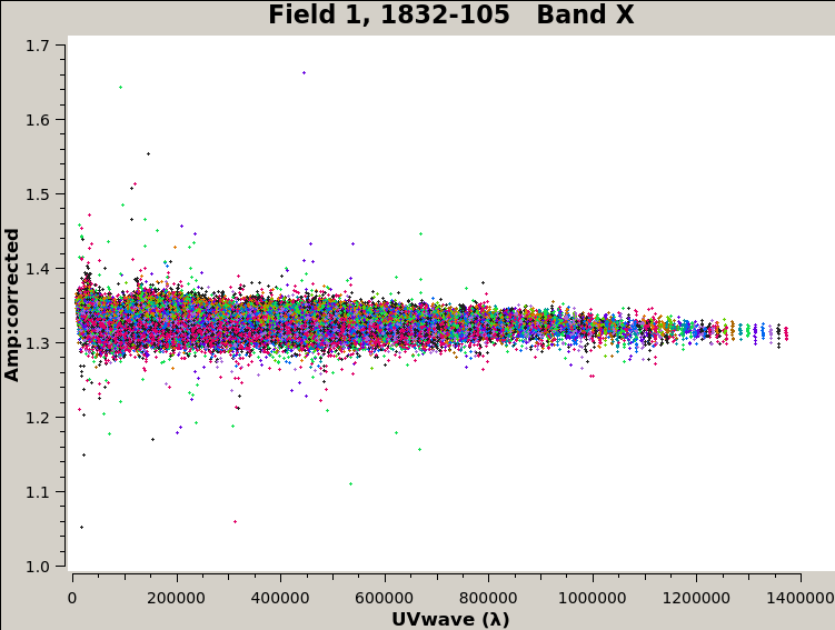
|[[Image:LongSolintFixed.png|400px|thumb|left|Fig. 8b. Corrected Amplitude vs UVwave for a complex gain calibrator taken in X-band, A-config. The observation used a long initial complex gain calibration scan to account for slew time. A section of the initial complex gain calibration scan was flagged in order to make the scan approximately as long as the other complex gain calibration scans. This resulted in the pipeline using a long solution interval of ~40s. Decorrelation is no longer evident.]] | |||
|} | |||
<pre style="white-space: pre-wrap; background-color: #E0FFFF;"> | <pre style="white-space: pre-wrap; background-color: #E0FFFF;"> | ||
| Line 101: | Line 155: | ||
== Weather == | == Weather == | ||
At the VLA, the weather has to meet certain conditions to run a scheduling block. The conditions vary with frequency and are more stringent for higher frequency observations (settable by the PI). It can happen, however, that the weather deteriorates after a scheduling block has started. High water vapor content and moving atmospheric cells can increase the system temperature and introduce extreme phase jumps. Wind (gusts) will also change the phase stability and cause more frequent pointing errors. Flagging times of bad weather conditions may help. The CASA task [https://casadocs.readthedocs.io/en/v6.2.1/api/tt/casatasks.manipulation.statwt.html statwt] will down-weight some noise variations. Also selfcal ([https://casaguides.nrao.edu/index.php/VLA_Self-calibration_Tutorial Topical Guide: VLA Self-calibration Tutorial]) will correct for phase variations. In extreme cases, however, flagging is the only method. | |||
For some SBs the weather data are missing from the header. This is usually not a big problem. The data can be filled, however, on request. Please contact the [https://help.nrao.edu NRAO helpdesk]. | For some SBs the weather data are missing from the header. This is usually not a big problem. The data can be filled, however, on request. Please contact the [https://help.nrao.edu NRAO helpdesk]. | ||
{| | |||
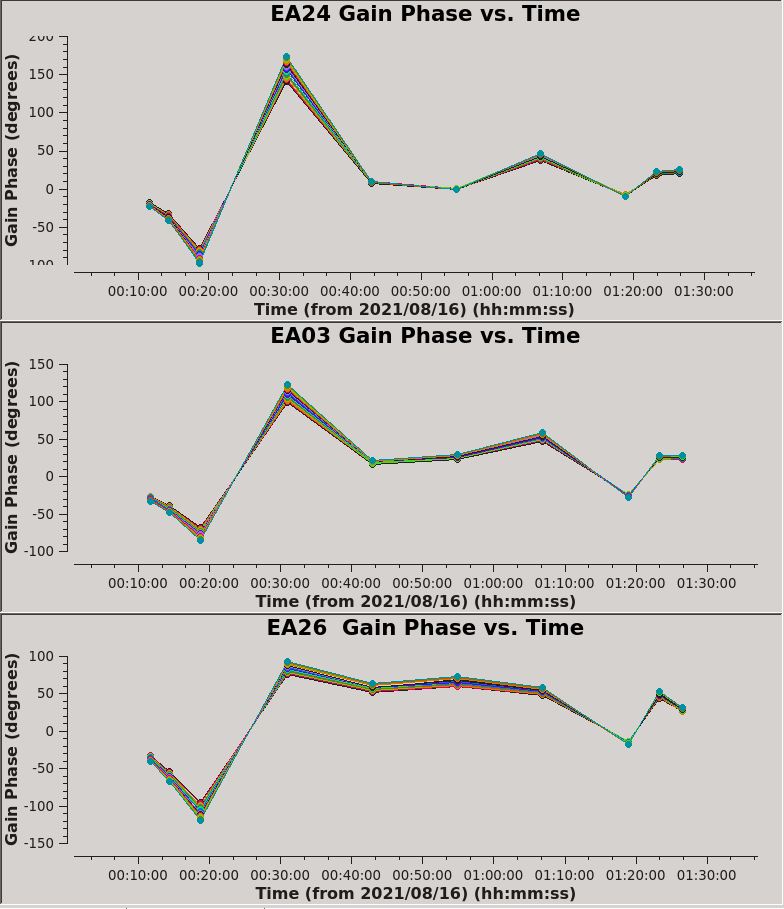
|[[Image:WestArmPhaseJump.png|400px|thumb|left|Fig. 9a. The phase solutions of the three outer most antennas on the West Arm during a B-config observation. A phase jump can be seen between 00:20:00 and 00:30:00. Often in the extended configurations one may notice the outer antennas on a particular arm of the array show such phase jumps as the weather can be significantly different between the outer and inner antennas as the array increases in size. Note that even if the jump is due to wrapping, there was a strong phase gradient at the beginning of the observations fiollowed by a much calmer period later.]] | |||
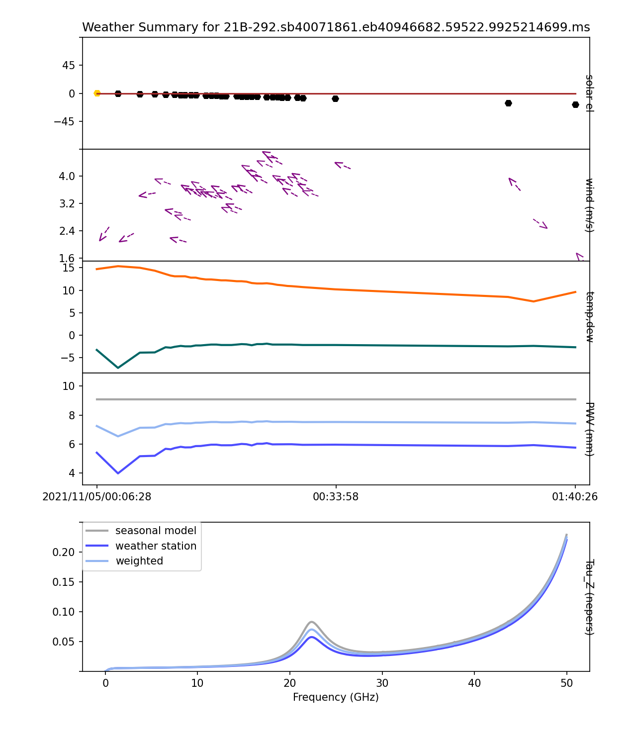
|[[Image:WeatherStationOutage.png|400px|thumb|right|Fig. 9b. A plot generated by the task plotweather which shows missing data. Such missing data is often due to power outages and glitches in the VLA's local weather monitoring station.]] | |||
|} | |||
<pre style="white-space: pre-wrap; background-color: #E0FFFF;"> | <pre style="white-space: pre-wrap; background-color: #E0FFFF;"> | ||
| Line 111: | Line 170: | ||
== Decorrelation == | == Decorrelation == | ||
The pipeline will correct for some degree of decorrelation for all calibrators. In extreme cases data need to be flagged | Decorrelation is an effect where the individual spatial frequencies of the visibilities are misaligned. If the misalignment is random the data is decorrelated, i.e., not all wave amplitudes are aligned, leading to destructive interference and thus a reduced amplitude. This effect is best seen in the plotsummary stage amplitude versus uv-wave plots. The biggest source of decorrelation is the atmosphere where a screen of a number of atmospheric cells with different refractive indices moves across the array, which causes errors in the delay and thus phase. The effect of decorrelation increases with observing time and is stronger for longer baselines. One correction for decorrelation is to increase the time between phase calibrator observations. At some time, however, decorrelation is constant (see the Advanced Calibration presentations at the [http://www.cvent.com/events/virtual-17th-synthesis-imaging-workshop/agenda-0d59eb6cd1474978bce811194b2ff961.aspx NRAO synthesis school]). | ||
The pipeline will correct for some degree of decorrelation for all calibrators. In extreme cases, however, data need to be flagged. If decorrelation is strong, it can be assumed that the target also shows significant decorrelation. Self-calibration is advised if the source flux is sufficient. A CASA guide for self-calibration is provided in the [https://casaguides.nrao.edu/index.php/VLA_Self-calibration_Tutorial Topical Guide: VLA Self-calibration Tutorial]. | |||
<pre style="white-space: pre-wrap; background-color: #E0FFFF;"> | <pre style="white-space: pre-wrap; background-color: #E0FFFF;"> | ||
FIX: Self-calibration. | FIX: Self-calibration. In extreme cases: flagging. | ||
</pre> | </pre> | ||
== Shadowing == | == Shadowing == | ||
The pipeline flags shadowed antennas by default. If not all of shadowing is captured, or if the shadowing criteria shall be loosened (e.g. allow a small amount of shadowing), then this can be controlled by the CASA task [https://casadocs.readthedocs.io/en/v6.2.1/api/tt/casatasks.flagging.flagdata.html flagdata] 'mode='shadow' . | The pipeline flags shadowed antennas by default. If not all of shadowing is captured, or if the shadowing criteria shall be loosened (e.g. allow a small amount of shadowing), then this can be controlled by the CASA task [https://casadocs.readthedocs.io/en/v6.2.1/api/tt/casatasks.flagging.flagdata.html flagdata] 'mode='shadow'. After manually flagging the data, he 'hifv_flagdata' task call should then be modified ('shadow=False') to not do additional shadowing flagging. | ||
<pre style="white-space: pre-wrap; background-color: #E0FFFF;"> | |||
FIX: in CASA: flagdata mode='shadow' | |||
</pre> | |||
== RFI plots look worse after Flagging== | |||
In some instances, the post-RFI flagging plots look aesthetically worse than the pre-RFI flagging plots. This is due to a poorly performing antenna (higher noise than others) that is getting heavily flagged in the RFI flagging. The post-RFI flagging plot then has less data to average together resulting in a worse looking plot. This is not a problem and the outcomes from imaging with and without the flagging of these poorly performing antennas are not scientifically different. In the case of these noisy data not getting flagged (as in the previous pipeline version), they are strongly down-weighted by statwt so they do not contribute much to the final images anyway. | |||
<pre style="white-space: pre-wrap; background-color: #E0FFFF;"> | |||
FIX: Nothing to fix, but inspect closely that this is only a plotting effect. | |||
</pre> | |||
== Delay differences == | |||
There's a known issue where in X-band the two polarizations show an offset of 16ns in their delays. This is not a problem as long as they are steady in frequency and will calibrate out. In general, delay differences larger than +/-10ns should be inspected and strong delay jumps due to RFI should be removed. | |||
<pre style="white-space: pre-wrap; background-color: #E0FFFF;"> | |||
FIX: Likely flagging for strong delay differences. Sometimes it is advisable to change to a different reference antenna. | |||
</pre> | |||
== System Issues == | |||
Sometimes, the calibration amplitude vs frequency or vs time plots show features resembling resonances, intermittent peaks or depressions, or swings (particularly in finalcals stage). A comparison with plotsummary will show if they calibrate out, or if there are residuals (non-symmetric noise in an antenna). If they are strong, maybe significantly more than 10%, antenna-specific flagging may be needed for bad basebands, spws or channels, or bad scans (potentially including the adjacent target scans). Then the calibration pipeline should be restarted. | |||
The issue has been identified in ea17 as being a loose cable on the C band receiver frontend. As of May 16, 2022, the issue should not appear anymore for that antenna in C band, but may still occur elsewhere. | |||
{| | |||
|[[Image:Switch3.png|400px|thumb|left|Fig. 10a. System issue that is manifested as a change in frequency in the amplitude-frequency calibration tables.]] | |||
|[[Image:switch2.png|400px|thumb|left|Fig. 10b. A second example of the system issue.]] | |||
|} | |||
<pre style="white-space: pre-wrap; background-color: #E0FFFF;"> | |||
FIX: Stronger features should be flagged. | |||
</pre> | |||
== Dynamic Range == | |||
If a source is very strong, systematic errors will be amplified and well visible in images. It is then difficult to deconvolve the sources and systematic errors may dominate well over the thermal rms noise levels. | |||
<pre style="white-space: pre-wrap; background-color: #E0FFFF;"> | |||
FIX: More careful calibration, additional calibration techniques such a position-dependent gain solutions, careful deconvolution, the use fo widefield or aw-projection gridders. Self-calibration. Generally such sources need to be treated by hand as the pipeline functions are limited. | |||
</pre> | |||
== Compression == | |||
Strong RFI can bring the digital and analog receiver system into a non-linear regime (also known as compression). This is especially a problem in L and S bands. Simple RFI flagging alone will not be sufficient to remove compression. The affected antennas/basebands will likely need to be flagged. | |||
There is a known local microwave antenna that emits in C band near 6.2 GHz. The signal is strong enough to cause compression on many antennas, especially in A and B configurations. This can be identified at several places in the weblog. Examples from a data set where ea18 was strongly affected are shown below. The spw containing 6.2 GHz has been flagged by the pipeline, while the rest of the upper baseband (C:A2C2 in this case) is clearly compressed. The lower baseband, C:A1C1, is in good condition. The signatures shown in the calibration table plots (Figs. 11c, 11d, 11e) may result from a number of issues (pointing, hardware, etc.) so they should be checked against switched power plots (Figs. 11a, 11b) to confirm compression as the cause. | |||
{| | |||
|[[Image:compression_SP_no.png|400px|thumb|left|Fig. 11a. priorcals > switched power<br />ea16 does NOT have compression and is shown here for comparison.]] | |||
|[[Image:compression_SP.png|400px|thumb|right|Fig #11b. priorcals > switched power.]] | |||
|} | |||
{| | |||
|[[Image:compression_BP.png|400px|thumb|left|Fig. 11c. finalcals > BP amp solution.]] | |||
|[[Image:compression_time.png|400px|thumb|Fig. 11d. finalcals > final amp time cal.]] | |||
|[[Image:compression_freq.png|400px|thumb|right|Fig. 11e. finalscals > final amp freq cal.]] | |||
|} | |||
For 8bit data, an algorithm that corrects for mild compression is available as a pipeline task. It has not been evaluated for 3bit data, however. | |||
<pre style="white-space: pre-wrap; background-color: #E0FFFF;"> | |||
FIX: For strong compression, flag the affected data. Weak compression may increase the Tsys. | |||
</pre> | |||
== Reverse spw index == | |||
A known issue will sometimes cause the indexing of spws to be in reverse frequency order within one or more basebands. This occurs when there is a bad baseline board resulting in a spw being excluded. This doesn't harm the data, but it can be misleading when reviewing a weblog. | |||
{| | |||
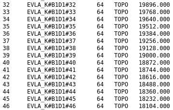
|[[File:Reverse_BD_listobs.png|400px|thumb|left|Fig. 12a. This setup normally has 16 spw per baseband. Within the B1D1 baseband there are only 15 spw, and as the index increases, frequency decreases.]] | |||
|[[File:Reverse_BD_plotsummary.png|400px|thumb|right|Fig. 12b. In plotsummary, spw are listed in numerical order, but in the plot spw 32 is on the right and spw 46 is on the left.]] | |||
|} | |||
<pre style="white-space: pre-wrap; background-color: #E0FFFF;"> | |||
FIX: No fix, just be aware when selecting spws. | |||
</pre> | |||
== OMT Reflection == | |||
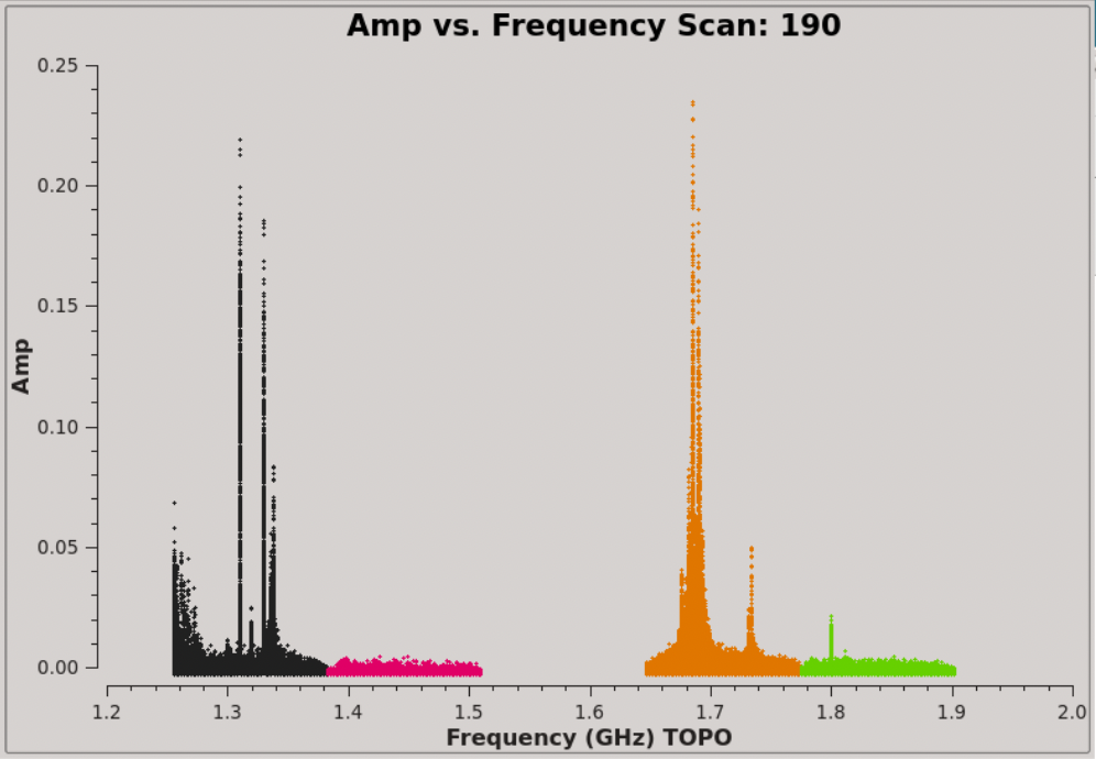
This appears as a sinusoidal pattern of the frequency plots of the calibrators in the 'plotsummary' stage, a residual after applying the bandpass tables. An explanation for this is moisture on the feedhorn window that allows standing waves within the feedhorn and the OMT. It is most common in late summer. | |||
{| | |||
|[[Image:Omt_reflection.png|400px|thumb|Fig. 13. A standing wave between the feed horn window and OMT causes a sinusoidal pattern across corrected amp vs freq.]] | |||
|} | |||
<pre style="white-space: pre-wrap; background-color: #E0FFFF;"> | |||
FIX: No specific fix for this effect, but check the fractional change of the sinusoidal pattern. For continuum it should mostly average out, otherwise it adds to the error budget. | |||
</pre> | |||
<!-- | |||
== Bug: Multi-band datasets missing high order spectral index coefficients == | |||
In fluxboot stage, when 3 or 4 spectral index coefficients are determined, a pipeline bug causes only the first 2 terms to be used when setting the calibrator models. Below is an example: | |||
{| | |||
|[[Image:coefficients.png|1200px|thumb|Fig. 14a. Spectral index coefficients table from fluxboot stage.]] | |||
|} | |||
The setjy call should be:<br /> | |||
setjy( vis='finalcalibrators.ms', field='1616-181', spw='2,3,4,5,6,7,8,9,10,11,12,13,14,15,16,17,18,19,20,21,22,23,24,25,26,27,28,29,30,31,32,33,34,35,36,37,38,39,40,41,42,43,44,45,46,47,48,49,50,51,52,53,54,55,56,57,58,59,60,61,62,63,64,65,66,67,68,69,70,71,72,73, | |||
74,75,76,77,78,79,80,81,82,83,84,85,86,87,88,89,90,91,92,93,94,95,96,97,98,99,100,101,102,103,104,105,106,107,108,109,110,111,112,113,114,115,116,117,118,119,120,121,122,123,124,125,126,127,128,129,130,131, | |||
132,133,134,135,136,137,138,139,140,141,142,143,144,145,146,147,148,149,150,151,152,153,154,155,156,157,158, | |||
159,160,161', | |||
selectdata=False, timerange='', scan='', intent='', observation='', scalebychan=True, standard='manual', model='', modimage='', listmodels=False, fluxdensity=[0.2525016089521427, 0.0, 0.0, 0.0], '''spix=[-0.11615064567962619, -0.33385703450504856, -0.07201862748125115, 0.42327948230992296]''', reffreq='14630590975.918522Hz', polindex=[], polangle=[], rotmeas=0.0, fluxdict={}, useephemdir=False, interpolation='nearest', usescratch=True, ismms=False )<br /> | |||
However, the bug causes only the first 2 terms to be used:<br /> | |||
'''spix=[-0.11615064567962619, -0.33385703450504856]'''<br /> | |||
Below are images comparing the gain calibrator model column after running setjy with 2 and 4 terms (these were manually plotted, not generated in pipeline weblog). | |||
{| | |||
|[[Image:model_2terms.jpg|400px|thumb|left|Fig. 14b. Gain calibrator model when only 2 terms are used.]] | |||
|[[Image:model_4terms.png|400px|thumb|right|Fig. 14c. Gain calibrator model when 4 terms are used.]] | |||
|} | |||
One symptom of the bug is a large a spread in gain solutions for the most affected bands, which will appear on all antennas. | |||
{| | |||
|[[Image:finalampfreqcal0_S_2terms.png|400px|thumb|left|Fig. 14d. Gain amp vs freq when only 2 terms are used.]] | |||
|[[Image:finalamptimecal0_S_2terms.png|400px|thumb|right|Fig. 14e. Gain amp vs time when only 2 terms are used.]] | |||
|} | |||
{| | |||
|[[Image:finalampfreqcal0_S_4terms.png|400px|thumb|left|Fig. 14f. Gain amp vs freq when 4 terms are used.]] | |||
|[[Image:finalamptimecal0_S_4terms.png|400px|thumb|right|Fig. 14g. Gain amp vs time when 4 terms are used.]] | |||
|} | |||
In this example S band is forced into a positive slope when it should be negative. This can result in the corrected amps being discontinuous between spws which looks like stairs/steps. | |||
{| | |||
|[[Image:spectral_index_fit.png|400px|thumb|left|Fig. 14h. Spectral index fit using all 4 spix terms. In S band (below 4 GHz on top X axis), the slope is clearly negative.]] | |||
|[[Image:discontinuous_spws.png|400px|thumb|right|Fig. 14i. Corrected amp vs freq for the phase calibrator in S band. Slopes within each spw are negative, but the overall slope across the band is positive because the model only used 2 spix terms instead of 4.]] | |||
|} | |||
<pre style="white-space: pre-wrap; background-color: #E0FFFF;"> | <pre style="white-space: pre-wrap; background-color: #E0FFFF;"> | ||
FIX: | FIX: This bug will be fixed in a future pipeline release. Manual setjy calls using all spix terms can done to bootstrap the gain calibrator models correctly. | ||
</pre> | </pre> | ||
== | --> | ||
== Flux calibrator models == | |||
<u>3C138 flare</u><br /> | |||
The flux density scale calibrator 3C138 has been undergoing a flare since at least mid-December 2020. At K and Ka-bands the magnitude of the flare is of order 40-50% compared to the Perley-Butler 2017 flux scale. The effect is smaller at lower frequencies (10-20% at C and X-band), and is larger at higher frequencies (more than a factor of two at Q-band).<br /> | |||
<pre style="white-space: pre-wrap; background-color: #E0FFFF;"> | <pre style="white-space: pre-wrap; background-color: #E0FFFF;"> | ||
FIX: | FIX: For flaring calibrators, monitoring datasets are publicly available in the archive under project code TCAL0009. From these observations, you may derive an updated flux density ratio to use for your observations. | ||
</pre> | </pre> | ||
<u>polarization calibration</u><br /> | |||
When one of the standard (as recognized by CASA) flux calibrator sources is used only for polarization angle calibration (or indeed any scan whose intents do NOT include flux calibration), its CASA model is not used, so the resulting amp vs uvwave plots are inaccurate. In the fluxboot stage, sometimes gain solutions may be missing for some basebands/spws of the pol cal. If the cal is used exclusively for polarization (not flux calibration), then this has no effect on the overall calibration for Stokes I.<br /> | |||
== | <pre style="white-space: pre-wrap; background-color: #E0FFFF;"> | ||
FIX: Before performing any polarization calibration we recommend setting the flux cal model image with setjy, then running gaincal on it with calmode='p'. | |||
</pre> | |||
<u>A configuration structure</u><br /> | |||
The current calibrator models for resolved flux density calibrators in A-configuration in CASA are created with narrow band data. At the high frequencies of a broad band observation, this can mean that the calibrator | |||
model does not represent the structure of the calibrator very well, leading to amplitude errors that reduce the dynamic range of the calibrated data. | |||
{| | |||
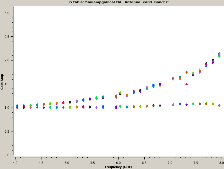
|[[Image:C_ramp_1.png|400px|thumb|left|Fig. 15a. finalcals > final amp freq cal. The phase cal solution increases across frequency, while the flux cal solution is flat near 1.0, due to the model issue.]] | |||
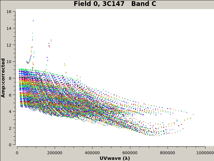
|[[Image:C_ramp_uvwave.png|400px|thumb|right|Fig. 15b. plotsummary. The uvwave plot for the flux cal shows amp spikes above 9 Jy due to the model issue.]] | |||
|} | |||
<pre style="white-space: pre-wrap; background-color: #E0FFFF;"> | |||
FIX: This will be remedied in a future version of CASA and the pipeline. If high image fidelity is required we have found that recalibration using a model for a higher frequency band scaled to the band of interest can work well. | |||
</pre> | |||
<u>Ka-band in A configuration</u><br /> | |||
The Ka-band models used for pipeline processing and packaged with CASA do not represent their sources in A-configuration very well, causing amplitude errors. | |||
{| | {| | ||
|[[Image: | |[[Image:3C286_model_issue.png|400px|thumb|left|Fig. 15c. Amp vs UVwave for 3C286 showing high amplitudes due to model issue.]] | ||
|[[Image:3C286_model_improved.png|400px|thumb|right|Fig. 15d. Amp vs UVwave for 3C286 using an improved model. New models will be released in a future version of casa.]] | |||
|} | |} | ||
<pre style="white-space: pre-wrap; background-color: #E0FFFF;"> | <pre style="white-space: pre-wrap; background-color: #E0FFFF;"> | ||
FIX: | FIX: New, more accurate models will be released with CASA in the future. | ||
</pre> | </pre> | ||
Latest revision as of 21:10, 12 September 2023
General Description
The VLA pipeline delivers calibrated data and some initial images of VLA observation runs. The quality of the calibration and imaging products is usually assessed through the weblog that is created in each pipeline run (see also the VLA Pipeline guide). During the observations, the VLA may have encountered technical problems that are reflected in various ways in the weblog, where graphs show the behavior of the calibration tables as a function of time, frequency, polarization, etc., and analytical numbers describe the amount of flagging, derived fluxes, image statistics, etc.
Here we would like to briefly describe common VLA observing problems, how they are identified in the pipeline calibration weblog, and how they can be addressed.
Radio Frequency Interference
By far the biggest problem is radio frequency interference (RFI). RFI is produced by internal and external sources, can be terrestrial or from satellites that operate at or spill into the observed frequency. For the VLA, please find more information on the Radio Frequency Interference webpage. Although weak RFI may only slightly raise the noise of an image with little influence on the calibration tables, stronger RFI will produce artifacts that may render the data (target and calibrators) unusable, if not adequately flagged. An example for strong RFI is shown below. Flagging procedures are outlined in the VLA topical CASA guide on flagging.
 |
It is important that all data are free of RFI.
FIX: Weak, intermittent RFI will increase the noise and be down-weighted in the imaging in the hifv_statwt task. Strong RFI needs to be flagged and only clean data should be calibrated and imaged. Flagging can be manual or automatic.
Pointing
At higher frequencies the VLA requires regular pointing calibrations. Each pointing run will reposition the antennas to be centered on a strong source with known position. If the pointing solution fails, the amplitude of the source will drop or drift away from the center of the antenna with the highest gain. A typical graph looks like the one shown below. The pointing solution for the first half of the run failed, which results in the source drifting away from the center of the primary beam. After a pointing update in the middle of the run, the antenna is positioned properly again (the very last data points are actually a different source, hence the drop at the edge).
 |
 |
FIX: If the pointing is only off by a small amount, the gain calibration will take care of it. If it is off by a large amount, the data for this period and antenna needs to be flagged.
Phase Jumps
Various hardware failures can cause the phase for a given antenna to be unstable in time, often with sudden, large changes in phase over time. Depending on where the problem is, this may affect just a portion of the data or up to all data on a given antenna. In the example below, only one baseband's data is affected (large changes at each data point) while the other baseband remains near zero and is not affected. This plot, from the pipeline's Final phase gain cal section found in the 'hifv_finalcals' stage, shows the final phase solutions found for each calibrator (using the long solution interval).
 |
Typical phase variations for low frequency data are a few degrees. For high frequencies tens of degrees can occur; the cycle time between the phase calibrator and the target needs to be reduced to adequately track and interpolate the phase variations as a function of time. If the phases vary more than 360 degrees between two phase calibrator scans, then the data are completely decorrelated and cannot be calibrated anymore (even changes larger than 180deg leave the interpolation pretty much undefined).
FIX: If there are phase jumps, usually the data for the affected time range needs to be flagged for the antenna(s).
DTS/Deformatter Problems
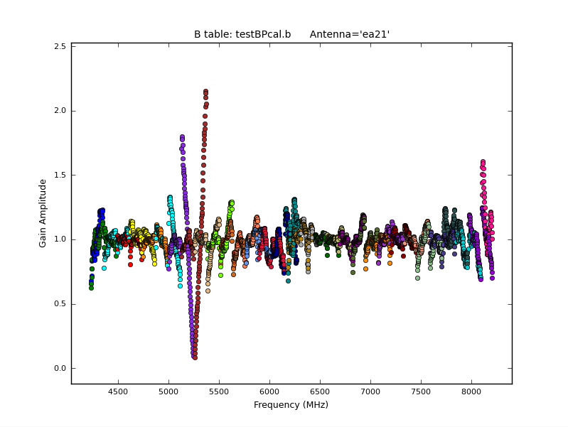
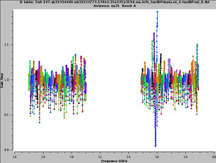
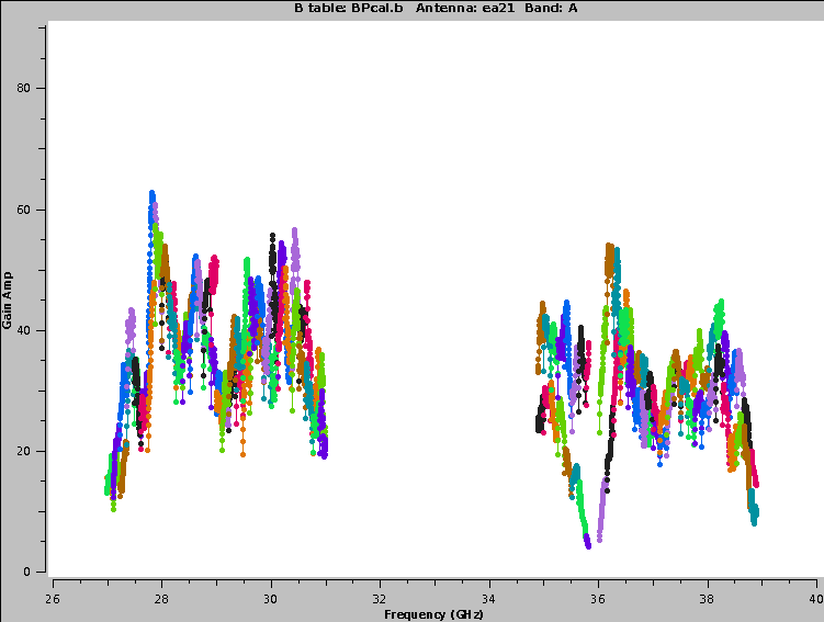
The digital transmission system (DTS) of each VLA antenna includes a formatting stage to convert the electronic signal to optical before it is injected on the optical fiber link. On the correlator end the signal will be deformatted back to an electronic signal. Occasionally the timing on the deformatter can be misaligned, which results in very strong amplitude or phase slopes as a function of frequency. When this occurs, the data are corrupt and the entire affected baseband per polarization of an antenna need to be flagged. Frequently the error shows up similar to an abs(sin) or a 'bouncing' signal across a baseband for one polarization or, in other terms, various numbers of 'V' shapes in the data, usually in the middle of a baseband.
 |
 |
 |
 |
Sometimes, however, the pipeline erroneously detects a DTS issue, when the data were in fact only affected by RFI in a few spws. If that happens it is better to flag the data manually, which preserves the rest of the baseband.
FIX: The data for this baseband, antenna and polarization need to be flagged.
Correlator Zeros
Under some circumstances, the WIDAR correlator writes exact zeros. The pipeline will usually flag them automatically. If not, they can be removed with CASA's flagdata task, using the option mode='clip' with clipzeros=True or flag the zeros by hand.
 |
The percentage is calculated based on channels. Spectral line spws are therefore more susceptible to a high reported number of zeros.
FIX: The pipeline will usually catch them. If not, use CASA's flagdata task.
Baseband and Subband Edges
If spw roll-off frequency edges are very steep, they can degrade gain and phase solutions. Frequently this is not a big problem, but if the gain for the edge channels is close to zero, a division by the bandpass for these channels can get extremely noisy. This is particularly true for baseband edges. The edgespw, fracspw, and baseband parameters in hifv_flagdata can be adjusted to flag different percentages of the edges (see also VLA pipeline pages). The edges can also be flagged with the CASA task flagdata, or by hand.
FIX: Adjust the relevant parameters in hifv_flagdata and re-run the pipeline.
Resolved Calibrators
Some calibrator sources are not perfect point sources. For the VLA standard flux calibrator sources, models are provided within CASA, which solves the problem for these. Resolved phase calibrators, however, will produce an more or less incorrect gaintable. In some cases, CASA's gaincal can even fail completely and set all fluxes to 1Jy. To work with resolved gain/phase calibrators, either provide a model, or, at least, restrict the uv-range to the unresolved portion during the solve. Plotting the amplitude against uv distance (uvwave) should clearly show the flat part that can be used, and the non-flat parts that should be omitted. Try to make sure though, that there are at least some baselines for every antenna available for the solve. Figures 6a and 6b show, respectively, the visibility data for an unresolved and a resolved calibrator.
A solution is to use the flux.csv table. It is usually generated for ALMA in a pipeline run, but can be created before a VLA run. The uv-ranges listed there will be used in the processing. The format is like:
ms,field,spw,I,Q,U,V,spix,uvmin,uvmax,comment
and an example entry would be:
MY.ms,0,2,1.0,0.0,0.0,0.0,0.0,21000.0,110000.0,"3C48"
for a uvrange of 21000-110000 lambda.
Above, ms is the MS name, field and spw are the IDs (not names, the ID will only be known once the data is in MS format and after executing listobs), I, Q, U, V are the Stokes flux densities in Jy (note that entries for the VLA will be ignored here, so a nominal I=1.0Jy will be ok), uvmin and uvmax are the uv ranges in units of lambda. Only one spw (the first) is used per field, other entries will be ignored. This means a single line entry such as the one above will apply to all spws for the given field. When using a uvrange, note that both a uvmin and uvmax must be specified: if one wants to specify only a uvmax, we suggest setting a uvmin of 0.01. If uvmax is provided as 0.0 lambda, then this creates an inequality and uvmax is unbounded.
If you have multi-band data, you may have to split the data per band first, then run each band through their own pipeline to make use of flux.csv.
FIX: Restrict the uv-range for the calculations of the calibration tables. The flux.csv table can be used.
Wrong Intents
If the intents of the data are set incorrectly for the observations, the pipeline will use the wrong calibrators for the calibration. Usually this can be fixed by overwriting the intents. The VLA pipeline webpage provides instructions and a script to do this. For more complicated setups, like multiple calibrators or bands with separate calibrator scans, data may be split into smaller MSs that contain only the relevant calibrators for each target, or data reduction by hand may be needed.
Non-ideal reference antenna
Sometimes if the reference antenna has some issue, like RFI or extreme flagging, it is advisable to switch to a different reference antenna. The example below shows that one spw has extreme phase jumps for all antennas when ea02 was chosen as a reference antenna (Fig. 7a). This indicates that the phase jumps are likely not present on all antennas, but that phase instabilities on ea02 itself are reflected on all other antennas. Indeed, when ea09 was chosen as a reference antenna, as shown in Fig. 7b, then the instability is shown only in ea02 and all other antennas are well-behaved. Delays are also a quantity that are relative to a chosen reference antenna. If the delays for all antennas show similarly high delays, then it is likely that the reference antenna has the high delays and not all other antennas. Chosing a different reference antenna would quickly reveal if this is the case.
Use the 'refantignore' keyword to disallow the use of this antenna as a reference (in the example one should ignore ea02 as a possible reference antenna). The Pipeline Page provides details on the usage of this keyword.
FIX: Use 'refantignore' to remove a problematic antenna from the list of possible reference antennas.
Extreme Solution Intervals
In the hifv_solint stage, the short solution interval is computed as the longest individual single integration (dump) of a visibility. The long solution interval is the longest scan on the gain/phase calibrator. If those values seem unreasonable, then the data should be inspected and flagged. Sometimes, the observations are set up with a long phase calibrator scan at the beginning, to allow for longer slews to the source. This can result in excessive long solints, and some flagging may be advised on this scan.
After flagging, the pipeline should then be re-run to determine new solution intervals.
FIX: Flagging bad data.
Weather
At the VLA, the weather has to meet certain conditions to run a scheduling block. The conditions vary with frequency and are more stringent for higher frequency observations (settable by the PI). It can happen, however, that the weather deteriorates after a scheduling block has started. High water vapor content and moving atmospheric cells can increase the system temperature and introduce extreme phase jumps. Wind (gusts) will also change the phase stability and cause more frequent pointing errors. Flagging times of bad weather conditions may help. The CASA task statwt will down-weight some noise variations. Also selfcal (Topical Guide: VLA Self-calibration Tutorial) will correct for phase variations. In extreme cases, however, flagging is the only method.
For some SBs the weather data are missing from the header. This is usually not a big problem. The data can be filled, however, on request. Please contact the NRAO helpdesk.
FIX: Statwt, selfcal, or flagging.
Decorrelation
Decorrelation is an effect where the individual spatial frequencies of the visibilities are misaligned. If the misalignment is random the data is decorrelated, i.e., not all wave amplitudes are aligned, leading to destructive interference and thus a reduced amplitude. This effect is best seen in the plotsummary stage amplitude versus uv-wave plots. The biggest source of decorrelation is the atmosphere where a screen of a number of atmospheric cells with different refractive indices moves across the array, which causes errors in the delay and thus phase. The effect of decorrelation increases with observing time and is stronger for longer baselines. One correction for decorrelation is to increase the time between phase calibrator observations. At some time, however, decorrelation is constant (see the Advanced Calibration presentations at the NRAO synthesis school).
The pipeline will correct for some degree of decorrelation for all calibrators. In extreme cases, however, data need to be flagged. If decorrelation is strong, it can be assumed that the target also shows significant decorrelation. Self-calibration is advised if the source flux is sufficient. A CASA guide for self-calibration is provided in the Topical Guide: VLA Self-calibration Tutorial.
FIX: Self-calibration. In extreme cases: flagging.
Shadowing
The pipeline flags shadowed antennas by default. If not all of shadowing is captured, or if the shadowing criteria shall be loosened (e.g. allow a small amount of shadowing), then this can be controlled by the CASA task flagdata 'mode='shadow'. After manually flagging the data, he 'hifv_flagdata' task call should then be modified ('shadow=False') to not do additional shadowing flagging.
FIX: in CASA: flagdata mode='shadow'
RFI plots look worse after Flagging
In some instances, the post-RFI flagging plots look aesthetically worse than the pre-RFI flagging plots. This is due to a poorly performing antenna (higher noise than others) that is getting heavily flagged in the RFI flagging. The post-RFI flagging plot then has less data to average together resulting in a worse looking plot. This is not a problem and the outcomes from imaging with and without the flagging of these poorly performing antennas are not scientifically different. In the case of these noisy data not getting flagged (as in the previous pipeline version), they are strongly down-weighted by statwt so they do not contribute much to the final images anyway.
FIX: Nothing to fix, but inspect closely that this is only a plotting effect.
Delay differences
There's a known issue where in X-band the two polarizations show an offset of 16ns in their delays. This is not a problem as long as they are steady in frequency and will calibrate out. In general, delay differences larger than +/-10ns should be inspected and strong delay jumps due to RFI should be removed.
FIX: Likely flagging for strong delay differences. Sometimes it is advisable to change to a different reference antenna.
System Issues
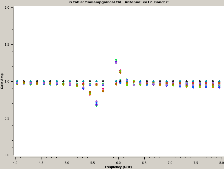
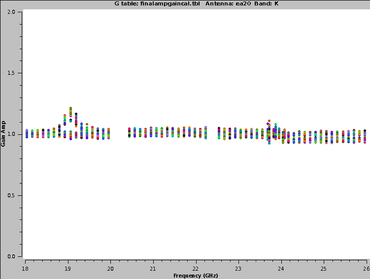
Sometimes, the calibration amplitude vs frequency or vs time plots show features resembling resonances, intermittent peaks or depressions, or swings (particularly in finalcals stage). A comparison with plotsummary will show if they calibrate out, or if there are residuals (non-symmetric noise in an antenna). If they are strong, maybe significantly more than 10%, antenna-specific flagging may be needed for bad basebands, spws or channels, or bad scans (potentially including the adjacent target scans). Then the calibration pipeline should be restarted.
The issue has been identified in ea17 as being a loose cable on the C band receiver frontend. As of May 16, 2022, the issue should not appear anymore for that antenna in C band, but may still occur elsewhere.
 |
 |
FIX: Stronger features should be flagged.
Dynamic Range
If a source is very strong, systematic errors will be amplified and well visible in images. It is then difficult to deconvolve the sources and systematic errors may dominate well over the thermal rms noise levels.
FIX: More careful calibration, additional calibration techniques such a position-dependent gain solutions, careful deconvolution, the use fo widefield or aw-projection gridders. Self-calibration. Generally such sources need to be treated by hand as the pipeline functions are limited.
Compression
Strong RFI can bring the digital and analog receiver system into a non-linear regime (also known as compression). This is especially a problem in L and S bands. Simple RFI flagging alone will not be sufficient to remove compression. The affected antennas/basebands will likely need to be flagged.
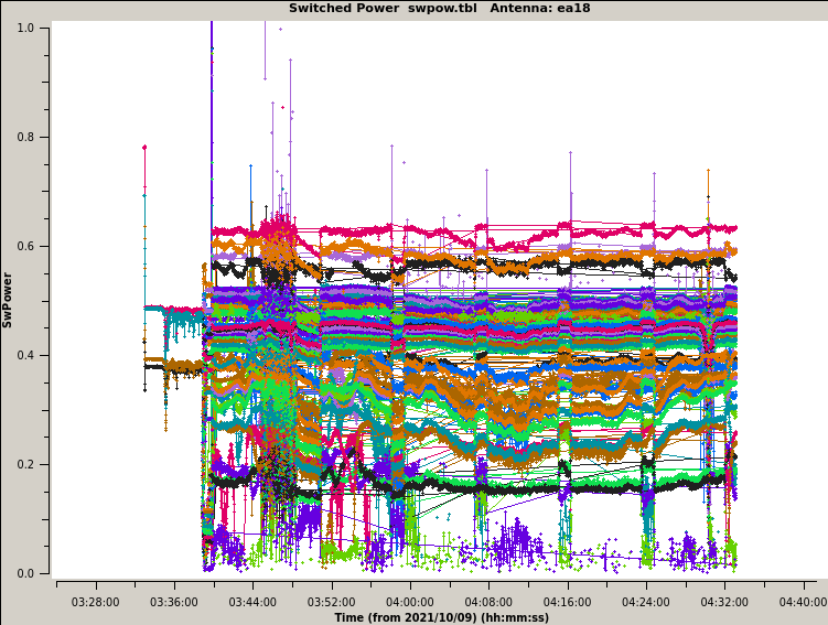
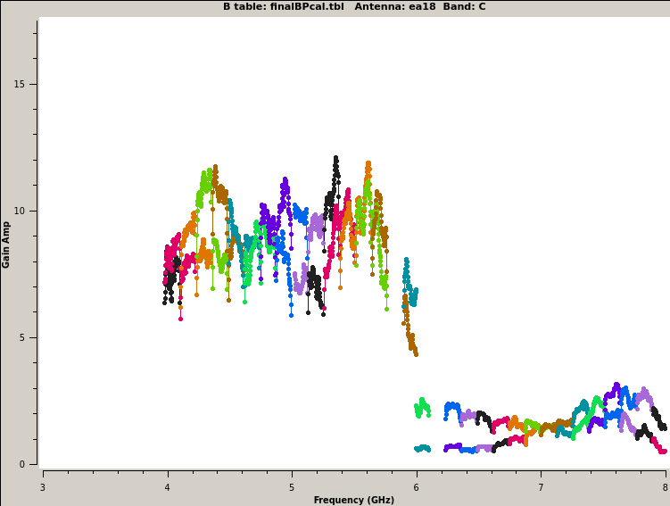
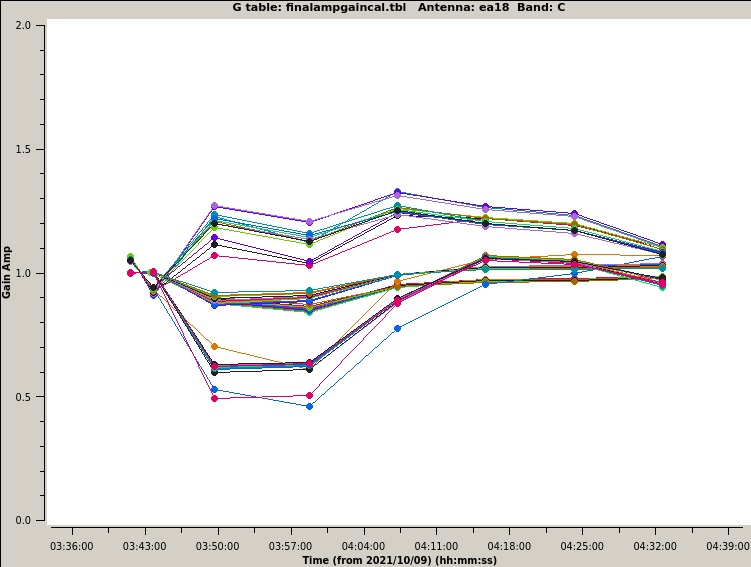
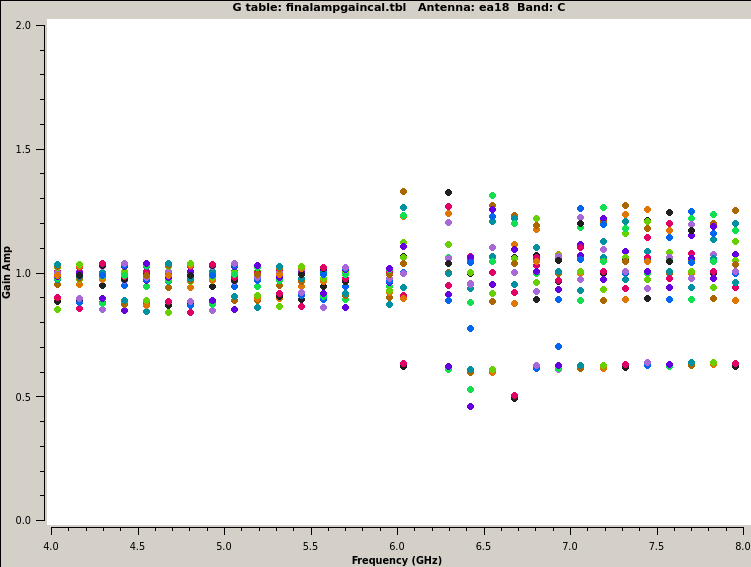
There is a known local microwave antenna that emits in C band near 6.2 GHz. The signal is strong enough to cause compression on many antennas, especially in A and B configurations. This can be identified at several places in the weblog. Examples from a data set where ea18 was strongly affected are shown below. The spw containing 6.2 GHz has been flagged by the pipeline, while the rest of the upper baseband (C:A2C2 in this case) is clearly compressed. The lower baseband, C:A1C1, is in good condition. The signatures shown in the calibration table plots (Figs. 11c, 11d, 11e) may result from a number of issues (pointing, hardware, etc.) so they should be checked against switched power plots (Figs. 11a, 11b) to confirm compression as the cause.
 ea16 does NOT have compression and is shown here for comparison. |
 |
 |
 |
 |
For 8bit data, an algorithm that corrects for mild compression is available as a pipeline task. It has not been evaluated for 3bit data, however.
FIX: For strong compression, flag the affected data. Weak compression may increase the Tsys.
Reverse spw index
A known issue will sometimes cause the indexing of spws to be in reverse frequency order within one or more basebands. This occurs when there is a bad baseline board resulting in a spw being excluded. This doesn't harm the data, but it can be misleading when reviewing a weblog.
FIX: No fix, just be aware when selecting spws.
OMT Reflection
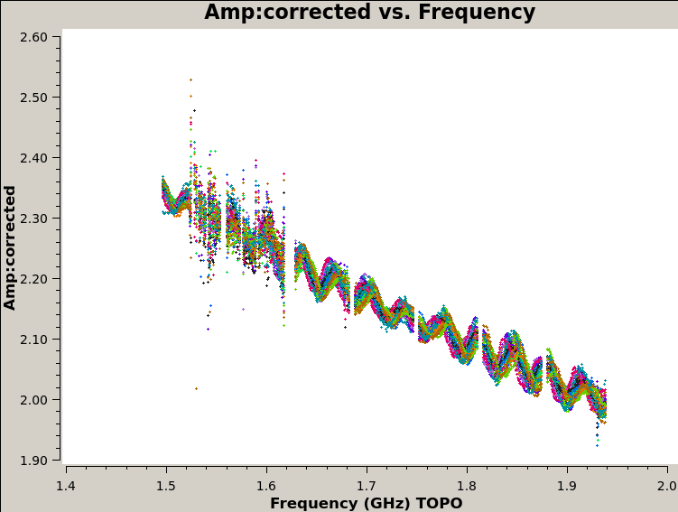
This appears as a sinusoidal pattern of the frequency plots of the calibrators in the 'plotsummary' stage, a residual after applying the bandpass tables. An explanation for this is moisture on the feedhorn window that allows standing waves within the feedhorn and the OMT. It is most common in late summer.
 |
FIX: No specific fix for this effect, but check the fractional change of the sinusoidal pattern. For continuum it should mostly average out, otherwise it adds to the error budget.
Flux calibrator models
3C138 flare
The flux density scale calibrator 3C138 has been undergoing a flare since at least mid-December 2020. At K and Ka-bands the magnitude of the flare is of order 40-50% compared to the Perley-Butler 2017 flux scale. The effect is smaller at lower frequencies (10-20% at C and X-band), and is larger at higher frequencies (more than a factor of two at Q-band).
FIX: For flaring calibrators, monitoring datasets are publicly available in the archive under project code TCAL0009. From these observations, you may derive an updated flux density ratio to use for your observations.
polarization calibration
When one of the standard (as recognized by CASA) flux calibrator sources is used only for polarization angle calibration (or indeed any scan whose intents do NOT include flux calibration), its CASA model is not used, so the resulting amp vs uvwave plots are inaccurate. In the fluxboot stage, sometimes gain solutions may be missing for some basebands/spws of the pol cal. If the cal is used exclusively for polarization (not flux calibration), then this has no effect on the overall calibration for Stokes I.
FIX: Before performing any polarization calibration we recommend setting the flux cal model image with setjy, then running gaincal on it with calmode='p'.
A configuration structure
The current calibrator models for resolved flux density calibrators in A-configuration in CASA are created with narrow band data. At the high frequencies of a broad band observation, this can mean that the calibrator
model does not represent the structure of the calibrator very well, leading to amplitude errors that reduce the dynamic range of the calibrated data.
FIX: This will be remedied in a future version of CASA and the pipeline. If high image fidelity is required we have found that recalibration using a model for a higher frequency band scaled to the band of interest can work well.
Ka-band in A configuration
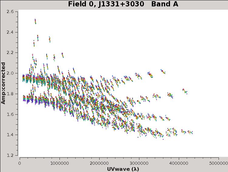
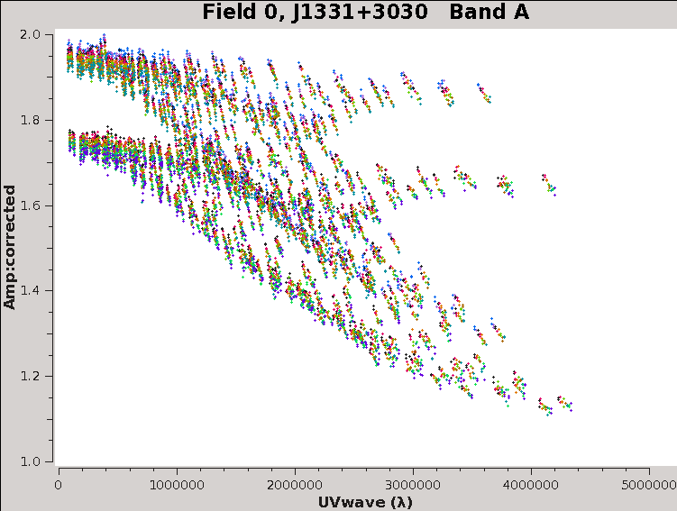
The Ka-band models used for pipeline processing and packaged with CASA do not represent their sources in A-configuration very well, causing amplitude errors.
 |
 |
FIX: New, more accurate models will be released with CASA in the future.
