Sunspot Band6 Feathering for CASA 5.1: Difference between revisions
No edit summary |
|||
| (10 intermediate revisions by 2 users not shown) | |||
| Line 1: | Line 1: | ||
[[Category:ALMA]][[Category:Imaging]][[Category:Sun]] | |||
==Overview== | ==Overview== | ||
| Line 23: | Line 25: | ||
# In Casa | # In Casa | ||
int_base = 'AR12470_B6AllSpw_I' # basename of the synthesized image | int_base = 'AR12470_B6AllSpw_I' # basename of the synthesized image | ||
sd_img_base = 'uid___A002_Xae00c5_X2e6b.PM03.StkI.Spw3 | sd_img_base = 'uid___A002_Xae00c5_X2e6b.PM03.StkI.Spw3' | ||
# basename of the full-sun map | # basename of the full-sun map | ||
out_base = 'AR12470_B6AllSpe_I_Feather' # basename of the final products | out_base = 'AR12470_B6AllSpe_I_Feather' # basename of the final products | ||
</source> | </source> | ||
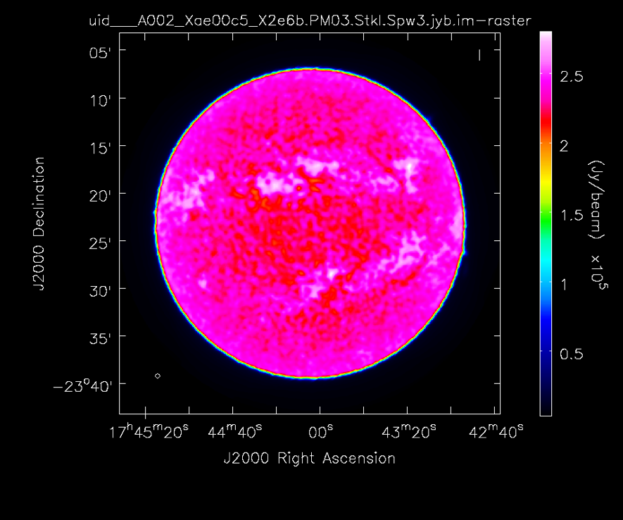
[[File:sunspot_fullsun2.png|thumb|right| | [[File:sunspot_fullsun2.png|thumb|right|'''Fig. 1.''' The full-sun map with ‘Jy/beam’ unit.]] | ||
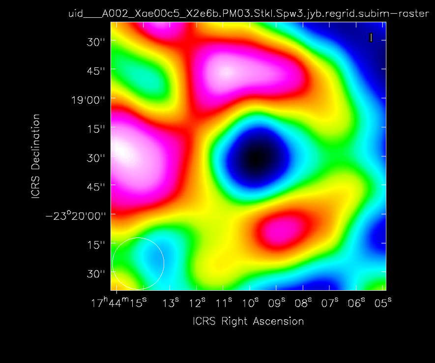
[[File:sunspot_sdspot.png|thumb|right| | [[File:sunspot_sdspot.png|thumb|right|'''Fig. 2.''' The trimmed map from the full-sun map.]] | ||
We shift the coordinate of the full-sun map created from the single-dish data, based on the RA/Dec coordinate obtained in the previous section, as follows. | We shift the coordinate of the full-sun map created from the single-dish data, based on the RA/Dec coordinate obtained in the previous section, as follows. | ||
<source lang='python'> | <source lang='python'> | ||
| Line 38: | Line 40: | ||
sun_ra = str(266.01898 * pi/180.) | sun_ra = str(266.01898 * pi/180.) | ||
sun_dec = str(-23.38648 * pi/180.) | sun_dec = str(-23.38648 * pi/180.) | ||
imhead(imagename = sd_img_base+'. | imhead(imagename = sd_img_base+'.rescl', mode = 'put', hdkey = 'crval1', hdvalue = sun_ra) | ||
imhead(imagename = sd_img_base+'. | imhead(imagename = sd_img_base+'.rescl', mode = 'put', hdkey = 'crval2', hdvalue = sun_dec) | ||
</source> | </source> | ||
The unit of the full-sun map is Kelvin. On the other hand, the unit of the synthesized image is Jy/beam. So, the conversion of the unit has to be done. In the tutorial, we convert the unit of the full-sun image to Jy/beam, using the following commands. | The unit of the full-sun map is Kelvin. On the other hand, the unit of the synthesized image is Jy/beam. So, the conversion of the unit has to be done. In the tutorial, we convert the unit of the full-sun image to Jy/beam, using the following commands. | ||
<source lang='python'> | <source lang='python'> | ||
# In Casa | # In Casa | ||
crval4S= imhead(sd_img_base+'. | crval4S= imhead(sd_img_base+'.rescl', mode='get',hdkey='crval4') | ||
freqSD = crval4S.values()[0] | freqSD = crval4S.values()[0] | ||
sbema = imhead(sd_img_base+'. | sbema = imhead(sd_img_base+'.rescl', mode='get',hdkey='beammajor') | ||
sbemi = imhead(sd_img_base+'. | sbemi = imhead(sd_img_base+'.rescl', mode='get',hdkey='beamminor') | ||
sbmajor = sbema.values()[0] | sbmajor = sbema.values()[0] | ||
sbminor = sbemi.values()[0] | sbminor = sbemi.values()[0] | ||
convKJb = str(13.6 * (300./(freqSD/1.e9))**2. * (1./sbmajor)*(1./sbminor)) | convKJb = str(13.6 * (300./(freqSD/1.e9))**2. * (1./sbmajor)*(1./sbminor)) | ||
immath(imagename=sd_img_base+'. | immath(imagename=sd_img_base+'.rescl', expr='IM0/'+convKJb, outfile=sd_img_base+'.jyb.im') | ||
imhead(imagename = sd_img_base+'.jyb.im', mode = 'put', hdkey = 'crval3', hdvalue = ['I']) | imhead(imagename = sd_img_base+'.jyb.im', mode = 'put', hdkey = 'crval3', hdvalue = ['I']) | ||
| Line 58: | Line 60: | ||
</source> | </source> | ||
The result of the process is shown in | The result of the process is shown in Figure 1. A look of the image is not changed, but you can find the changing of the values and unit in the ‘Sunspot_Band6_SingleDish_for_CASA_4.7’ tutorial. | ||
Then we do the re-gridding and trimming to fit the map area to that of the synthesized image. The area of the trimming is set to the same as the CLEAN box, in the tutorial. | Then we do the re-gridding and trimming to fit the map area to that of the synthesized image. The area of the trimming is set to the same as the CLEAN box, in the tutorial. | ||
| Line 78: | Line 80: | ||
==Preparation for Feathering task: The Synthesized image== | ==Preparation for Feathering task: The Synthesized image== | ||
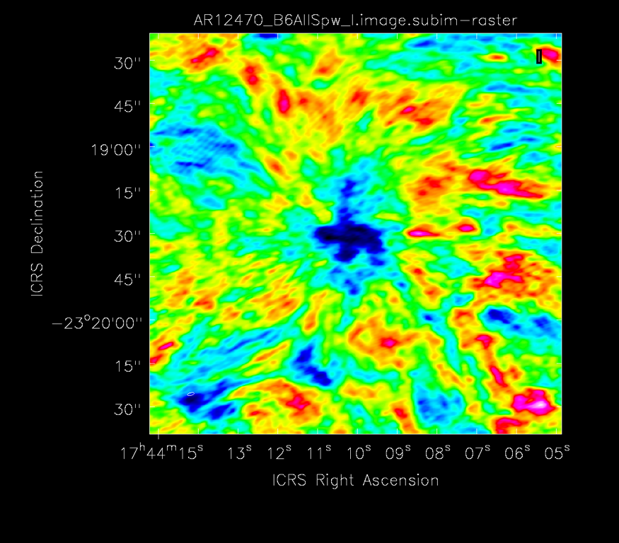
[[File:sunspot_syntrim.png|thumb|right| | [[File:sunspot_syntrim.png|thumb|right|'''Fig. 3''' The trimmed map from the synthesized image.]] | ||
To fit the map area to that of the trimmed single-dish image, we do the trimming for the synthesized image. | To fit the map area to that of the trimmed single-dish image, we do the trimming for the synthesized image. | ||
<source lang='python'> | <source lang='python'> | ||
| Line 90: | Line 92: | ||
The combining of the maps can be done using ‘feathering’ task, as the same as the non-solar data. | The combining of the maps can be done using ‘feathering’ task, as the same as the non-solar data. | ||
<source lang='python'> | <source lang='python'> | ||
# In CASA | |||
feather(imagename=out_base+'.image', highres=int_base+'.image.subim',lowres=sd_img_base+'.jyb.regrid.subim.depb') | feather(imagename=out_base+'.image', highres=int_base+'.image.subim',lowres=sd_img_base+'.jyb.regrid.subim.depb') | ||
</source> | </source> | ||
| Line 101: | Line 104: | ||
</source> | </source> | ||
To convert the unit from Jy/beam to Kelvin, we use the following commands. | To convert the unit from Jy/beam to Kelvin, we use the following commands. | ||
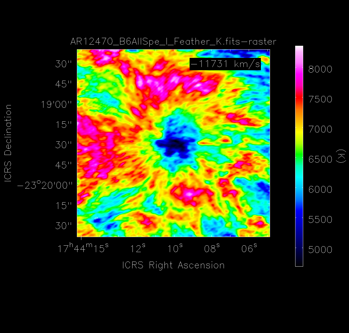
[[File:sunspot_final.png|thumb|right| | [[File:sunspot_final.png|thumb|right|'''Fig. 4.''' The trimmed map from the synthesized image.]] | ||
<source lang='python'> | <source lang='python'> | ||
# In Casa | # In Casa | ||
| Line 125: | Line 128: | ||
</source> | </source> | ||
The result of the combining is shown in | The result of the combining is shown in Figure 4. | ||
---- | |||
'''Caution: The single-dish images and feathering images in the solar SV data packages (ex. Sunspot_Band6_ReferenceImages.tgz) were not applied the re-scaling to the single-dish data (see [[Sunspot_Band6_SingleDish_for_CASA_5.1#Calibration_.28re-scaling.29_after_Imaging]]). Please do not use the reference image for your science.''' | |||
Latest revision as of 20:42, 19 August 2021
Overview
This portion of the Sunspot Band6 CASA Guide for CASA 5.1 covers the combine process between the synthesized solar image and the full-sun image obtained with TP array. It begins where the calibration of the visibility data and single-dish data, image synthesis, and creating of the full-sun map are completed. If you do not complete them, at first,
1) Download the file of the un-calibrated data package ‘Sunspot_Band6_UncalibratedData.tgz’, do the calibration of the data, and create the images from the interferometric data and single-dish data, along with the ‘Sunspot_Band6_*_for_CASA_5.1’ tutorials.
or
2) Download the file of the calibrated data package ‘Sunspot_Band6_CalibratedData.tgz’, and synthesize the image from interferometric data along the ‘Sunspot_Band6_Imaging_for_CASA_5.1’ tutorial.
In case 1), we assume that you are working on the working directory ‘Sunspot_Band6_UncalibratedData’. On the other hand, when you started the tutorial from the calibrated package (case 2), we assume that the working directory is ‘Sunspot_Band6_CalibratedData.’
From next, we will show all commands for combining the images.
Obtaining the RA/Dec coordinate of the sun center at the reference time
Before starting the combination process on CASA, we need to know the RA/Dec coordinate of the sun center at the reference time that is used for the image synthesis, because the observing time of the TP-array is not the same as the reference time exactly. The Sun was moving on the RA/Dec coordinate frame during the gap between the times. To combine the synthesized image with the full-sun image obtained from the TP array, we need to shift the coordinate of the full-sun image based on the coordinate of the sun center at the reference time. Hence, we obtain the solar coordinate from the JPL’s HORIZONS system[1].
The reference time in this tutorial is 19:49:00UT, December 18 2015. At the time, the RA/Dec coordinate of the sun center estimated by JPL’s HORIZONS system is RA: 266.01898 degree, Dec: -23.38648 degrees.
Preparation for Feathering task: The Single-Dish data
We start the process on CASA by defining some names of the data.
# In Casa
int_base = 'AR12470_B6AllSpw_I' # basename of the synthesized image
sd_img_base = 'uid___A002_Xae00c5_X2e6b.PM03.StkI.Spw3'
# basename of the full-sun map
out_base = 'AR12470_B6AllSpe_I_Feather' # basename of the final products


We shift the coordinate of the full-sun map created from the single-dish data, based on the RA/Dec coordinate obtained in the previous section, as follows.
# In Casa
sun_ra  = str(266.01898 * pi/180.)
sun_dec = str(-23.38648 * pi/180.)
imhead(imagename = sd_img_base+'.rescl', mode = 'put', hdkey = 'crval1', hdvalue = sun_ra)
imhead(imagename = sd_img_base+'.rescl', mode = 'put', hdkey = 'crval2', hdvalue = sun_dec)
The unit of the full-sun map is Kelvin. On the other hand, the unit of the synthesized image is Jy/beam. So, the conversion of the unit has to be done. In the tutorial, we convert the unit of the full-sun image to Jy/beam, using the following commands.
# In Casa
crval4S= imhead(sd_img_base+'.rescl', mode='get',hdkey='crval4')
freqSD = crval4S.values()[0]
sbema = imhead(sd_img_base+'.rescl', mode='get',hdkey='beammajor')
sbemi = imhead(sd_img_base+'.rescl', mode='get',hdkey='beamminor')
sbmajor = sbema.values()[0]
sbminor = sbemi.values()[0]
convKJb = str(13.6 * (300./(freqSD/1.e9))**2. * (1./sbmajor)*(1./sbminor))

immath(imagename=sd_img_base+'.rescl', expr='IM0/'+convKJb, outfile=sd_img_base+'.jyb.im')

imhead(imagename = sd_img_base+'.jyb.im', mode = 'put', hdkey = 'crval3', hdvalue = ['I'])
imhead(imagename = sd_img_base+'.jyb.im', mode = 'put', hdkey = 'bunit', hdvalue = 'Jy/beam')
The result of the process is shown in Figure 1. A look of the image is not changed, but you can find the changing of the values and unit in the ‘Sunspot_Band6_SingleDish_for_CASA_4.7’ tutorial.
Then we do the re-gridding and trimming to fit the map area to that of the synthesized image. The area of the trimming is set to the same as the CLEAN box, in the tutorial.
# In Casa
#re-griding of SD data
imregrid(imagename=sd_img_base+'.jyb.im', template=int_base+'.image', axes=[0, 1], output=sd_img_base+'.jyb.regrid')

# Trimming to exclude noisy edge regions in the TP image
imsubimage(imagename=sd_img_base+'.jyb.regrid', outfile=sd_img_base+'.jyb.regrid.subim', box='555,565,1505,1490')
As the final process of the preparation of the single-dish data, we multiply the trimmed image by the primary beam response, as follows.
# In Casa
imsubimage(imagename=int_base+'.flux',outfile=int_base+'.flux.subim',box='555,565,1505,1490')

immath(imagename=[sd_img_base+'.jyb.regrid.subim',int_base+'.flux.subim'], expr='IM0*IM1', outfile=sd_img_base+'.jyb.regrid.subim.depb')
Preparation for Feathering task: The Synthesized image

To fit the map area to that of the trimmed single-dish image, we do the trimming for the synthesized image.
# In Casa
imsubimage(imagename=int_base+'.image', outfile=int_base+'.image.subim', box='555,565,1505,1490')
Combining, primary beam correction, and creating of the FITS file.
The combining of the maps can be done using ‘feathering’ task, as the same as the non-solar data.
# In CASA
feather(imagename=out_base+'.image', highres=int_base+'.image.subim',lowres=sd_img_base+'.jyb.regrid.subim.depb')
CAUTION: In this tutorial and the packages of the solar SV data released on 2017/01/18, we use the default parameters of the task, as shown above. As a result, the averaged brightness temperature of the combined image is always larger a few % than the temperature brightness at the same position in the single-dish map, although the values have to be the same basically. It means that you need to tune the “sdfactor" parameter of the task for obtaining consistent images, before using combined images for your science. The detail of the parameter is described in Section 5.6 of “CASA User Reference & Cookbook Release 4.7.0”[2].
After the feathering process, we do the primary beam correction, as follows.
# In Casa
impbcor(imagename=out_base+'.image', pbimage=int_base+'.flux.subim', outfile=out_base+'.pbcor', mode='divide')
To convert the unit from Jy/beam to Kelvin, we use the following commands.

# In Casa
crval4I= imhead(int_base+'.image', mode='get',hdkey='crval4')
freq = crval4I.values()[0]
fbema = imhead(out_base+'.image', mode='get',hdkey='beammajor')
fbemi = imhead(out_base+'.image', mode='get',hdkey='beamminor')
fbmajor = fbema.values()[0]
fbminor = fbemi.values()[0]

convKJb2 =  str(13.6 * (300./(freq/1.e9))**2. * (1./fbmajor)*(1./fbminor))

immath(imagename=out_base+'.pbcor',expr='IM0*'+convKJb2, outfile= out_base+'_K.pbcor')

imhead(imagename = out_base+'_K.pbcor', mode = 'put', hdkey = 'bunit', hdvalue = 'K')
Finally, we create the FITS file of the combined and primary corrected map.
# In Casa
exportfits(imagename=out_base+'_K.pbcor', fitsimage=out_base+'_K.fits')
The result of the combining is shown in Figure 4.
Caution: The single-dish images and feathering images in the solar SV data packages (ex. Sunspot_Band6_ReferenceImages.tgz) were not applied the re-scaling to the single-dish data (see Sunspot_Band6_SingleDish_for_CASA_5.1#Calibration_.28re-scaling.29_after_Imaging). Please do not use the reference image for your science.