AIPS-Simple-Self-Cal: Difference between revisions
| (67 intermediate revisions by 7 users not shown) | |||
| Line 7: | Line 7: | ||
*Perform self-calibration to improve the imaging | *Perform self-calibration to improve the imaging | ||
This guide only | This guide only gives the important inputs to each task. The other inputs should be default. An easy way to set all the inputs to the default in a task is to type "default ''taskname''". | ||
== AIPS == | == AIPS == | ||
| Line 13: | Line 13: | ||
For a comprehensive overview of AIPS see the [http://www.aips.nrao.edu/CookHTML/CookBook.html AIPS COOKBOOK], especially [http://www.aips.nrao.edu/CookHTML/CookBookch3.html#x20-240003 Chapter 3:Basic AIPS Utilities] and [http://www.aips.nrao.edu/CookHTML/CookBookch12.html#x107-31300012 Chapter 12:AIPS for the More Sophisticated User]for the basics. [http://www.aips.nrao.edu/CookHTML/CookBookch9.html#x87-2010009 Chapter 9:Reducing VLBI Data in AIPS] is the chapter explaining VLBI data reduction, but it is rather overwhelming so [http://www.aips.nrao.edu/CookHTML/CookBookap3.html#x171-401000C Appendix C:A Step-by-Step Recipe for VLBA Data Calibration in AIPS] is recommended as a first step. However, below I summarize some useful commands (in parenthesis are the short form of the command): | For a comprehensive overview of AIPS see the [http://www.aips.nrao.edu/CookHTML/CookBook.html AIPS COOKBOOK], especially [http://www.aips.nrao.edu/CookHTML/CookBookch3.html#x20-240003 Chapter 3:Basic AIPS Utilities] and [http://www.aips.nrao.edu/CookHTML/CookBookch12.html#x107-31300012 Chapter 12:AIPS for the More Sophisticated User]for the basics. [http://www.aips.nrao.edu/CookHTML/CookBookch9.html#x87-2010009 Chapter 9:Reducing VLBI Data in AIPS] is the chapter explaining VLBI data reduction, but it is rather overwhelming so [http://www.aips.nrao.edu/CookHTML/CookBookap3.html#x171-401000C Appendix C:A Step-by-Step Recipe for VLBA Data Calibration in AIPS] is recommended as a first step. However, below I summarize some useful commands (in parenthesis are the short form of the command): | ||
*getname (getn) ''catalog #'': get the name of catalog # and put in INNAME, INCLASS and INSEQ. Other similar: geton (get outname); get2n (get in2name); get3n ( | *getname (getn) ''catalog #'': get the name of catalog # and put in INNAME, INCLASS and INSEQ. Other similar: geton (get outname); get2n (get in2name); get3n (get in3name) etc.. | ||
*input (inp) ''taskname'': show the inputs of taskname. | *input (inp) ''taskname'': show the inputs of taskname. | ||
*tget ''taskname'': get a task and fill in the inputs of the last time the task was run, one of the most useful commands in AIPS. | *tget ''taskname'': get a task and fill in the inputs of the last time the task was run, one of the most useful commands in AIPS. | ||
| Line 22: | Line 22: | ||
*imhead (imh): Print the file header (this can be used on both uv data and images despite the name). This will list informative things like the date of observation and the number and types of tables attached to the data. | *imhead (imh): Print the file header (this can be used on both uv data and images despite the name). This will list informative things like the date of observation and the number and types of tables attached to the data. | ||
== Getting the Data == | == Getting the Data and Other Useful Files == | ||
To obtain | To obtain these files, right click on the desired file below and select "Save Link As...": | ||
*[ | *[http://www.aips.nrao.edu/FITS/VLBA/bl193bg_3sour_avg.fits bl193bg_3sour_avg.fits] (543 MB): Data we will be reducing today. | ||
*[http://www.aips.nrao.edu/FITS/VLBA/1828_1.box 1828_1.box]: Box file for imaging. | |||
*[http://www.aips.nrao.edu/FITS/VLBA/1828_2.box 1828_2.box]: Box file for imaging. | |||
*[http://www.aips.nrao.edu/FITS/VLBA/1828_3.box 1828_3.box]: Box file for imaging. | |||
*[http://www.aips.nrao.edu/FITS/VLBA/1828_4.box 1828_4.box]: Box file for imaging. | |||
Files you might want to get in case something goes wrong with the primary calibration or if you just want to try the imaging and self-calibration: | |||
*[http://www.aips.nrao.edu/FITS/VLBA/0851+202.SPLIT.1 0851+202.SPLIT.1] (6.3 MB): Calibrated data for source 0851+202. | |||
*[http://www.aips.nrao.edu/FITS/VLBA/1828+487.SPLIT.1 1828+487.SPLIT.1] (7.8 MB): Calibrated data for source 1828+487. | |||
*[http://www.aips.nrao.edu/FITS/VLBA/2200+420.SPLIT.1 2200+420.SPLIT.1] (6.8 MB): Calibrated data for source 2200+420. | |||
If that doesn't work you can also ftp the data using anonymous ftp: | If that doesn't work you can also ftp the data using anonymous ftp: | ||
| Line 31: | Line 40: | ||
*cd pub/SIW | *cd pub/SIW | ||
*get bl193bg_3sour_avg.fits | *get bl193bg_3sour_avg.fits | ||
*mget *.box | |||
and optionally | |||
*mget *.SPLIT.1 | |||
The best place to put | The best place to put these files is in your $FITS area. This is an AIPS data area that should already have an environmental variable set up for it. | ||
== About the Data == | == About the Data == | ||
This is part of an observation from the [http://www.physics.purdue.edu/MOJAVE/index.html MOJAVE] survey | This is part of an observation from the [http://www.physics.purdue.edu/MOJAVE/index.html MOJAVE] survey, which is a large project that uses the VLBA to monitor Active Galactic Nuclei at 15 GHz in total and polarized flux. This project has been monitoring AGN for over a decade. The observation we are using took place on 16 June 2016 and contained 22 sources. However, in order to make the data a manageable size for a data reduction tutorial, three sources have been copied out of the dataset and the frequency channels and sample times have both been averaged by a factor of two. The sources in the the bl193bg_3sour_avg.fits dataset are as follows: | ||
*0851+202 - BL Lac object, bright source with not a lot of structure, used as bandpass calibrator, aka OJ287. [http://www.physics.purdue.edu/astro/MOJAVE/sourcepages/0851+202.shtml MOJAVE source page] | *0851+202 - BL Lac object, bright source with not a lot of structure, used as bandpass calibrator, aka OJ287. [http://www.physics.purdue.edu/astro/MOJAVE/sourcepages/0851+202.shtml MOJAVE source page] | ||
| Line 48: | Line 60: | ||
=== Starting AIPS === | === Starting AIPS === | ||
Start AIPS by typing '''aips''' or possibly '''aips tv=local:0.0''' in a terminal window. Depending on your AIPS installation, you might be prompted to pick a printer, then you will be asked for an AIPS number, if you are not sharing disks with anyone pick any number other than 1. Remember that number because the data you load and work on will be under that number. ''It would be best for this tutorial for you to use a clean AIPS number, in other words, an AIPS number that you have not used for anything else and has no data loaded into it.'' | Start AIPS by typing '''aips''' or possibly '''aips tv=local:0.0''' in a terminal window. Depending on your AIPS installation, you might be prompted to pick a printer, then you will be asked for an AIPS number, if you are not sharing disks with anyone pick any number other than 1. Remember that number because the data you load and work on will be under that number. ''It would be best for this tutorial for you to use a clean AIPS number, in other words, an AIPS number that you have not used for anything else and that has no data loaded into it.'' | ||
After AIPS has started type: | |||
* dowait=1 | |||
This means that AIPS will not allow you to run more than one task at a time. I usually run with dowait=-1; but for this tutorial and for beginners it is better to set dowait=1. | |||
=== Loading Data Into AIPS === | === Loading Data Into AIPS === | ||
Load the data with [http://www.aips.nrao.edu/cgi-bin/ZXHLP2.PL?FITLD '''FITLD''']. Note that I am forcing an outname, outclass and outseq, we are doing it here so it will be easy to | Load the data with [http://www.aips.nrao.edu/cgi-bin/ZXHLP2.PL?FITLD '''FITLD''']. Note that I am forcing an outname, outclass and outseq, we are doing it here so it will be easy to talk about specific files. | ||
First load the target and calibrators | First load the target and calibrators | ||
# default fitld | # default fitld | ||
# clint 0.25 ➜ set CL table interval to 15 seconds. | # clint 0.25 ➜ set CL table interval to 15 seconds. | ||
# datain ' | # datain 'MYAIP:bl193bg_3sour_avg.fits ➜ Two things to note: 1) this assumes that the data is in the $MYAIP directory, you can use a full directory path (e.g., datain '/home/mydata/bl193bg_3sour_avg.fits) or another environmental variable if the data is elsewhere (if the directory path is too long then you will get an error, to remedy this you may also use 'PWD:bl193bg_3sour_avg.fits); 2) The lack of a close ' is not a typo, you must leave off the closing ' or AIPS will capitalize everything within the ' ' and you will get an error because FITLD will not be able to find the data. | ||
# outname 'bl193bg' | # outname 'bl193bg' | ||
# outclass 'uvdata' | # outclass 'uvdata' | ||
| Line 80: | Line 97: | ||
=== Preliminary Data Evaluation === | === Preliminary Data Evaluation === | ||
Look at the structure of the data with [http://www.aips.nrao.edu/cgi-bin/ZXHLP2.PL?LISTR'''LISTR''']. This will give you a listing of the scans as well as the sources and frequency structure in the observation. Note that even though this dataset contains only three sources, the SU (source) table still contains all the sources in the original dataset, so LISTR will list all the sources and show 0 | Look at the structure of the data with [http://www.aips.nrao.edu/cgi-bin/ZXHLP2.PL?LISTR'''LISTR''']. This will give you a listing of the scans as well as the sources and frequency structure in the observation. Note that even though this dataset contains only three sources, the SU (source) table still contains all the sources in the original dataset, so LISTR will list all the sources and show 0 visibilities for the sources with no data. | ||
# default listr | # default listr | ||
| Line 93: | Line 110: | ||
=== Data Reduction Procedure === | === Data Reduction Procedure === | ||
Load in the VLBA data reduction procedures: see [http://www.aips.nrao.edu/cgi-bin/ZXHLP2.PL?VLBAUTIL EXPLAIN VLBAUTIL] for full description of procedures. | Load in the VLBA data reduction procedures: see [http://www.aips.nrao.edu/cgi-bin/ZXHLP2.PL?VLBAUTIL EXPLAIN VLBAUTIL] for a full description of the numerous procedures. | ||
Procedures are run by just typing their name, rather than using "go". | Procedures are run by just typing their name, rather than using "go". | ||
| Line 105: | Line 122: | ||
Data observed at 8 GHz or lower frequencies may be effected by the dispersive delay caused by the ionosphere. This will distort images and is especially bad at very low frequencies. An ionospheric correction based on maps of the electron content of the ionosphere can be performed with [http://www.aips.nrao.edu/cgi-bin/ZXHLP2.PL?VLBATECR '''VLBATECR''']. ''BL193BG is observed at 15 GHz so no ionospheric correction is needed.'' | Data observed at 8 GHz or lower frequencies may be effected by the dispersive delay caused by the ionosphere. This will distort images and is especially bad at very low frequencies. An ionospheric correction based on maps of the electron content of the ionosphere can be performed with [http://www.aips.nrao.edu/cgi-bin/ZXHLP2.PL?VLBATECR '''VLBATECR''']. ''BL193BG is observed at 15 GHz so no ionospheric correction is needed.'' | ||
Data using phase referencing can be | Data using phase referencing can be affected by imprecise Earth Orientation Parameters (EOPs) used in correlation. Therefore all phase referenced data should have its EOPs corrected. This can be done with [http://www.aips.nrao.edu/cgi-bin/ZXHLP2.PL?VLBAEOPS '''VLBAEOPS''']. ''BL193BG does not use phase referencing so no EOP correction is needed.'' | ||
=== Apply Digital Sampling Correction to VLBA data === | === Apply Digital Sampling Correction to VLBA data === | ||
Correct sampler threshold errors from correlator by running [http://www.aips.nrao.edu/cgi-bin/ZXHLP2.PL?VLBACCOR '''VLBACCOR''']. | Correct sampler threshold errors from the correlator by running [http://www.aips.nrao.edu/cgi-bin/ZXHLP2.PL?VLBACCOR '''VLBACCOR''']. | ||
# default vlbaccor | # default vlbaccor | ||
| Line 116: | Line 133: | ||
# vlbaccor | # vlbaccor | ||
VLBACCOR runs [http://www.aips.nrao.edu/cgi-bin/ZXHLP2.PL?ACCOR '''ACCOR'''] which creates | VLBACCOR runs [http://www.aips.nrao.edu/cgi-bin/ZXHLP2.PL?ACCOR '''ACCOR'''] which creates a solution (SN) table, then smooths the table with [http://www.aips.nrao.edu/cgi-bin/ZXHLP2.PL?SNSMO '''SNSMO'''], and then runs [http://www.aips.nrao.edu/cgi-bin/ZXHLP2.PL?CLCAL '''CLCAL'''] to apply the solutions to the calibration (CL) table. When VLBACCOR is finished you should get messages like those below that tell you what SN table and CL table are created. It is a good idea to save these messages. | ||
<pre> | <pre> | ||
| Line 127: | Line 144: | ||
[[Image:0851_possm1.png|250px|thumb|right|'''Figure 1''' <br /> Plot of amplitudes (bottom) and phases (top) for source 0851+202.]] | [[Image:0851_possm1.png|250px|thumb|right|'''Figure 1''' <br /> Plot of amplitudes (bottom) and phases (top) for source 0851+202.]] | ||
Now lets take a look at the fringe finders by running [http://www.aips.nrao.edu/cgi-bin/ZXHLP2.PL?VLBACRPL '''VLBACRPL''']. VLBACRPL runs [http://www.aips.nrao.edu/cgi-bin/ZXHLP2.PL?POSSM '''POSSM'''] and displays the spectrum of each baseline (to Fort Davis | Now lets take a look at the fringe finders by running [http://www.aips.nrao.edu/cgi-bin/ZXHLP2.PL?VLBACRPL '''VLBACRPL''']. VLBACRPL runs [http://www.aips.nrao.edu/cgi-bin/ZXHLP2.PL?POSSM '''POSSM'''] and displays the spectrum of each baseline (to Fort Davis which is antenna 2), with the amplitude on the bottom and the phases on the top. | ||
# default vlbacrpl | # default vlbacrpl | ||
| Line 148: | Line 165: | ||
</pre> | </pre> | ||
So hit A if you want to look at a plot longer than the 30 seconds, B or C to go to the next plot, D to exit. | So hit A if you want to look at a plot longer than the 30 seconds, B or C to go to the next plot, D to exit. | ||
You can look at the antennas through AIPS to find a nice reference antenna (refant; here as antenna 2) by running "go prtan". | |||
=== Determine Delay Corrections === | === Determine Delay Corrections === | ||
| Line 157: | Line 176: | ||
#default vlbapcor | #default vlbapcor | ||
#getn 1 | #getn 1 | ||
#calsour '0851+202' | #calsour '0851+202' ' | ||
#timer 0 19 26 33 0 19 36 38 ➜ scan with good fringes on all telescopes we found in POSSM plots. | #timer 0 19 26 33 0 19 36 38 ➜ scan with good fringes on all telescopes we found in POSSM plots. | ||
#refant 2 ➜ choose reference antenna from in the middle of array, antenna 2 or FD (Fort Davis, TX) is a good choice. | #refant 2 ➜ choose reference antenna from in the middle of array, antenna 2 or FD (Fort Davis, TX) is a good choice. | ||
| Line 164: | Line 183: | ||
#vlbapcor | #vlbapcor | ||
At this point you should check on the calibration: | (Note that the second quote sign ' after the source name causes all other values of CALSOUR to be blank.) At this point you should check on the calibration: | ||
*VLBAPCOR runs PCCOR which used the pulse cals to correct the intrumental phases and then runs CLCAL to apply the solutions to the CL (calbration table). The output from '''VLBAPCOR''' will look something like this: | *VLBAPCOR runs PCCOR which used the pulse cals to correct the intrumental phases and then runs CLCAL to apply the solutions to the CL (calbration table). The output from '''VLBAPCOR''' will look something like this: | ||
| Line 208: | Line 227: | ||
# default vlbabpss | # default vlbabpss | ||
# getn 1 | # getn 1 | ||
# calsour '0851+202' ➜ use | # calsour '0851+202' ' ➜ use a strong source as the bandpass calibrator. | ||
# refant 2 | # refant 2 | ||
# inp | # inp | ||
| Line 267: | Line 286: | ||
# go | # go | ||
Figure 4 shows the amplitude gains change over time as the sources rise and set, with higher gains at lower elevations. The different IFs and polarizations (RR and LL in this case) are shown as different colors. | Figure 4 shows that the amplitude gains change over time as the sources rise and set, with higher gains at lower elevations. The different IFs and polarizations (RR and LL in this case) are shown as different colors. | ||
=== Correct Phases for Parallactic Angles === | === Correct Phases for Parallactic Angles === | ||
| Line 288: | Line 307: | ||
[[Image:EDITR3.png|250px|thumb|right|'''Figure 6''' <br /> To flag this data we click FLAG TIME RANGE and hit B, and a blue box appears in the 01-10 box on the bottom.]] | [[Image:EDITR3.png|250px|thumb|right|'''Figure 6''' <br /> To flag this data we click FLAG TIME RANGE and hit B, and a blue box appears in the 01-10 box on the bottom.]] | ||
[[Image:EDITR4.png|250px|thumb|right|'''Figure 7''' <br /> After moving the sides of the box to encompass the data that need to be flagged, hit C and the data | [[Image:EDITR4.png|250px|thumb|right|'''Figure 7''' <br /> After moving the sides of the box to encompass the data that need to be flagged, hit C and the data are flagged and turn red.]] | ||
| Line 300: | Line 319: | ||
# doband 1 | # doband 1 | ||
# bpver 1 | # bpver 1 | ||
# antuse 1 2 3 4 5 6 7 8 9 10 ➜ to plot all the baselines to one antenna at the same time. | # antuse 1 2 3 4 5 6 7 8 9 10 ➜ to plot all the baselines to one antenna at the same time. | ||
| Line 310: | Line 327: | ||
*#go | *#go | ||
Again look in you terminal window for | Again look in you terminal window for instructions: | ||
<pre> | <pre> | ||
EDITR1: Press buttons A, B, or C to choose an operation | EDITR1: Press buttons A, B, or C to choose an operation | ||
| Line 316: | Line 333: | ||
</pre> | </pre> | ||
EDITR plots both amplitudes and phases verses time, so this is a good way to just look at your data. For the inputs we chose all the polarizations and IFs are plotted on top of each other. The two boxes on the bottom | EDITR plots both amplitudes and phases verses time, so this is a good way to just look at your data. For the inputs we chose, all the polarizations and IFs are plotted on top of each other. The two boxes on the bottom plot these as different colors and show the amplitude and phase for one baseline. The other boxes, where the data are shown in green, are the other baselines to that single antenna. It is especially useful to look at the data this way because problems tend to be antenna based so all the baselines to an antenna will be effected. It you see potentially problematic data (especially high or low amplitudes or with bad phases (note that weak sources will have incoherent phases)), then you should wait to flag until you can see all the baselines to the other antenna in the baseline pair with the bad data. That way you can flag once, telling EDITR to flag all the data for one antenna (this is the default in EDITR, but can be changed). The data for this source looks great. Click "NEXT ANTENNA" found on the menu to the right and press "B" until you have looked at all the baselines on all the antennas for this source. At this point the data has been amplitude calibrated but the source amplitude changes from scan to scan, do you know the reason for this? | ||
Now plot the other sources and inspect. | Now plot the other sources and inspect. | ||
| Line 330: | Line 347: | ||
*#go | *#go | ||
As you can see in Figure 5 this source the first scan on the baselines to antenna 10 looks bad. The amplitude is very low and the phases are noise. To flag this data click FLAG TIME RANGE and hit B (Figure 6), and a blue box appears in the 01-10 box on the bottom. By hitting A and moving the cursor move the sides of the box to encompass the data which needs to be flagged; then hit C. The data will be flagged on all the baselines to the antenna and will turn red in the display (Figure 7). | As you can see in Figure 5 this source the first scan on the baselines to antenna 10 looks bad. The amplitude is very low and the phases are noise. To flag this data click FLAG TIME RANGE and hit B (Figure 6), and a blue box appears in the 01-10 box on the bottom. By hitting A and moving the cursor move the sides of the box to encompass the data which needs to be flagged; then hit C. The data will be flagged on all the baselines to the antenna and will turn white in the lower colored parts and red in the upper comparison parts of the display (Figure 7). | ||
=== Fringe Fit the Data === | === Fringe Fit the Data === | ||
Perform a global fringe fit with [http://www.aips.nrao.edu/cgi-bin/ZXHLP2.PL?FRING '''FRING''']. The following steps through imaging are not strictly necessary since we will have to redo them once the geodetic calibration is done, but | Perform a global fringe fit with [http://www.aips.nrao.edu/cgi-bin/ZXHLP2.PL?FRING '''FRING''']. The following steps through imaging are not strictly necessary since we will have to redo them once the geodetic calibration is done, but they are an excellent way to check that the calibration up to this point is correct. | ||
# default fring | # default fring | ||
| Line 357: | Line 373: | ||
FRING1: Adjusting solutions to a common reference antenna | FRING1: Adjusting solutions to a common reference antenna | ||
</pre> | </pre> | ||
You should get something similar but not necessarily exactly the same numbers of good and failed solutions. A small percentage of failed solutions are fine at this point. FRING will have created SN table number 5. | You should get something similar, but not necessarily exactly the same numbers of good and failed solutions. A small percentage of failed solutions are fine at this point. FRING will have created SN table number 5. | ||
Since we did not use a source model, FRING assumes that the calibration source is a point source at the phase center. None of these sources are point sources. Therefore the corrections FRING finds will not correct the data perfectly and, once we apply all the calibration, it will be necessary to do self-calibration with source models to get the best images. Also note that I said "at the phase center" so, no matter what the the true position of your target, this fringe fit will move the brightest spot of the source to the phase center (the position of the target in the correlation). | |||
=== Apply FRING solutions === | === Apply FRING solutions === | ||
Note that the previous step and this step can be done in the single procedure [http://www.aips.nrao.edu/cgi-bin/ZXHLP2.PL?VLBAFRNG '''VLBAFRNG''']. It is broken up here just | Note that the previous step and this step can be done in the single procedure [http://www.aips.nrao.edu/cgi-bin/ZXHLP2.PL?VLBAFRNG '''VLBAFRNG''']. It is broken up here just to show both the steps explicitly, but also because running the tasks individually allows for more control. Here the global fringe fit which was done in the last step is interpolated and applied to the all the calibration that has gone before with [http://www.aips.nrao.edu/cgi-bin/ZXHLP2.PL?CLCAL '''CLCAL''']. | ||
# default clcal | # default clcal | ||
| Line 377: | Line 393: | ||
# go | # go | ||
So SN table #5 will be applied to CL table #6 and | So SN table #5 will be applied to CL table #6 and create CL table #7 which now includes all the calibration. | ||
=== Backing up Your Calibration === | === Backing up Your Calibration === | ||
We will want to save the calibration up to this point with [http://www.aips.nrao.edu/cgi-bin/ZXHLP2.PL?TASAV '''TASAV''']. TASAV makes a new file with all your calibration tables | We will want to save the calibration up to this point with [http://www.aips.nrao.edu/cgi-bin/ZXHLP2.PL?TASAV '''TASAV''']. TASAV makes a new file with all your calibration tables. This is very useful because it contains everything you need to recalibrate your data in a very compact and portable form. It is also a good idea to do this before you do anything you are unsure about or will change important tables (AN, SU) in ways that are hard to change back. | ||
# default tasav | # default tasav | ||
| Line 398: | Line 414: | ||
AIPS 1: 2 193 BL193BG .TASAV . 1 UV 27-JUN-17 11:52:14 | AIPS 1: 2 193 BL193BG .TASAV . 1 UV 27-JUN-17 11:52:14 | ||
</pre> | </pre> | ||
Note that you now have a second catalog entry which TASAV | Note that you now have a second catalog entry which TASAV automatically named BL193BG.TASAV.1. This uv data file has 1 visibility and all the tables attached to BL193BG.UVDATA.1. Lets look at the TASAVed file.: | ||
#getn 2 | #getn 2 | ||
#imh | #imh | ||
| Line 448: | Line 464: | ||
# getn 1 | # getn 1 | ||
# freqid 0 | # freqid 0 | ||
# docal 1; gainu 7 ➜ apply calibration; from CL# | # docal 1; gainu 7 ➜ apply calibration; from CL#7. | ||
# sour '0851+202', '1828+487', '2200+420' | # sour '0851+202', '1828+487', '2200+420' | ||
# doband 1; bpver 1 | # doband 1; bpver 1 | ||
| Line 465: | Line 481: | ||
AIPS 1: 5 193 1828+487 .SPLIT . 1 UV 03-JUL-17 15:15:29 | AIPS 1: 5 193 1828+487 .SPLIT . 1 UV 03-JUL-17 15:15:29 | ||
</pre> | </pre> | ||
=== OPTIONAL: Getting the Calibrated Data === | |||
'''''THIS STEP IS OPTIONAL: If everything went well in the above steps there is no need to get the calibrated data.''''' | |||
However If something went wrong with the calibration or if you want to start with the imaging and self-calibration then download the following files and put them in your $FITS area: | |||
*[http://www.aips.nrao.edu/FITS/VLBA/0851+202.SPLIT.1 0851+202.SPLIT.1] (6.3 MB): Calibrated data for source 0851+202. | |||
*[http://www.aips.nrao.edu/FITS/VLBA/1828+487.SPLIT.1 1828+487.SPLIT.1] (7.8 MB): Calibrated data for source 1828+487. | |||
*[http://www.aips.nrao.edu/FITS/VLBA/2200+420.SPLIT.1 2200+420.SPLIT.1] (6.8 MB): Calibrated data for source 2200+420. | |||
Then load the data with [http://www.aips.nrao.edu/cgi-bin/ZXHLP2.PL?FITLD '''FITLD''']: | |||
# default fitld | |||
# datain 'MYAIP:0851+202.SPLIT.1 | |||
# outdisk 1 | |||
# inp | |||
# go | |||
and repeat for 1828+487.SPLIT.1 and 2200+420.SPLIT.1. | |||
'''Note that these data do not include self-calibration but does include flagging.''' | |||
=== Flagging 1828+487 === | === Flagging 1828+487 === | ||
| Line 471: | Line 507: | ||
[[Image:WIPER3.png|250px|thumb|right|'''Figure 10''' <br /> WIPER plot with low amp points flagged (in blue).]] | [[Image:WIPER3.png|250px|thumb|right|'''Figure 10''' <br /> WIPER plot with low amp points flagged (in blue).]] | ||
Let's do some more flagging before we get into imaging. A nice graphical flagging task that is especially useful after SPLITing is [http://www.aips.nrao.edu/cgi-bin/ZXHLP2.PL?WIPER '''WIPER''']. WIPER defaults to plot amplitude vs uv distance: | |||
# default wiper | # default wiper | ||
| Line 479: | Line 515: | ||
# go | # go | ||
Ick! Look at those high points (Figure 8). Flag those by clicking on FLAG AREA, setting a box hitting the "A" key then hitting the "C" key when done, the flaged points will turn blue as in Figure 9. Now click EXIT and hit "A". Immediately type "go" to run WIPER again. This is more like it (Figure 10), but there are some low points, flag those with FLAG AREA but don't be too | Ick! Look at those high points (Figure 8). Flag those by clicking on FLAG AREA, setting a box hitting the "A" key then hitting the "C" key when done, the flaged points will turn blue as in Figure 9. Now click EXIT and hit "A". Immediately type "go" to run WIPER again. This is more like it (Figure 10), but there are some low points, flag those with FLAG AREA but don't be too overzealous. | ||
Now you have 2 flag (FG) tables attached to the data, one for each run of WIPER. FG table 2 has all the flags in it. | Now you have 2 flag (FG) tables attached to the data, one for each run of WIPER. FG table 2 has all the flags in it. | ||
=== Imaging and Self-Cal | === Imaging and Self-Cal of 1828+487 === | ||
[[Image:IMAGR1.png|250px|thumb|right|'''Figure 11''' <br /> Dirty map of 1828+487.]] | |||
[[Image:IMAGR2.png|250px|thumb|right|'''Figure 12''' <br /> Residual map of 1828+487.]] | |||
[[Image:IMAGR3.png|250px|thumb|right|'''Figure 13''' <br /> Image of 1828+487 after first run of IMAGR.]] | |||
Lets start by imaging 1828+487 with [http://www.aips.nrao.edu/cgi-bin/ZXHLP2.PL?IMAGR '''IMAGR''']. Either use the clean box files provided (make sure they are in the $MYAIP directory) or do interactive boxing. Using the supplied box file is easier. Also lets make sure that dowait=1 by typing: | |||
* dowait=1 | |||
Note that I came up with the parameters below especially the IMSIZE, ROBUST, RASH and DECSH by imaging and experimenting. | |||
Task [http://www.aips.nrao.edu/cgi-bin/ZXHLP2.PL?SETFC '''SETFC'''] can be used to recommend CELLSIZE and IMSIZE if you specify a desired field of view. The shifts were chosen, for this source only, to center the object including its jet within the image. | |||
It is recommended that you use the supplied box files. They reflect both the very obvious emission in the field and additional information from the MOJAVE project. | |||
# default imagr | # default imagr | ||
# getn 5 | # getn 5 | ||
# cell 0.0001; imsi 1024 512 ➜ cell size of 0.1 mas; image size of | # cell 0.0001; imsi 1024 512 ➜ cell size of 0.1 mas; image size of 1024x512. | ||
# rash -0.0125 0 | # rash -0.0125 0 | ||
# decsh 0.0125 0 | # decsh 0.0125 0 | ||
| Line 499: | Line 540: | ||
# robust 5 ➜ Do natural weighting. This source has a big diffuse jet, therefore sensitivity and more weight on the short spacings is more important than high resolution. | # robust 5 ➜ Do natural weighting. This source has a big diffuse jet, therefore sensitivity and more weight on the short spacings is more important than high resolution. | ||
# niter 5000 ➜ do interactive clean; with 5000 iterations, you will probably "stop cleaning" before hitting 5000 on the first iteration of imaging. | # niter 5000 ➜ do interactive clean; with 5000 iterations, you will probably "stop cleaning" before hitting 5000 on the first iteration of imaging. | ||
# boxfile ' | # boxfile 'MYAIP:1828_1.box | ||
# inp | # inp | ||
# go | # go | ||
# recat | |||
Hit TVPSEUDO then "B" immediately to get color rather than grey scale. Figure 11 shows the dirty map. If you want to clean interactively, then click CONTINUE CLEAN (and "A"); after a few rounds of cleaning (about 300 clean components which the messages from IMAGR tell you) the residuals will look like Figure 12. You can see in Figure 12 there is not much else to clean inside the clean boxes although there is some flux outside the clean boxes. This isn't significant enough to box at this point, so click STOP CLEANING ("A"). IMAGR will return the cleaned map, Figure 13, as you can see there are artifacts in the map. | |||
Once IMAGR is done you run [http://www.aips.nrao.edu/cgi-bin/ZXHLP2.PL?RECAT '''RECAT'''], which compresses the catalog so there are no empty spaces. This is not strictly necessary, but to follow this tutorial and have the GETN work, we have to be sure that the catalog numbers are consistent. Now do a [http://www.aips.nrao.edu/cgi-bin/ZXHLP2.PL?MCAT '''mcat'''] (mc for short) to look at the maps in your catalog: | |||
*mc | *mc | ||
<pre> | <pre> | ||
| Line 512: | Line 556: | ||
AIPS 1: 7 195 1828+487 .ICL001. 1 MA 04-JUL-17 10:33:14 | AIPS 1: 7 195 1828+487 .ICL001. 1 MA 04-JUL-17 10:33:14 | ||
</pre> | </pre> | ||
Note that you have made two | Note that you have made two files, a "dirty beam" (the IBM001 file) and a cleaned map (ICL001). | ||
To look at the image use [http://www.aips.nrao.edu/cgi-bin/ZXHLP2.PL?TVLOD '''TVLOD'''] (getn 6; tvin; tvlo). Use [http://www.aips.nrao.edu/cgi-bin/ZXHLP2.PL?TVPSEUDO '''TVPSEUDO'''] to put it into color (tvps). You can | To look at the image use [http://www.aips.nrao.edu/cgi-bin/ZXHLP2.PL?TVLOD '''TVLOD'''] (getn 6; tvin; tvlo). Use [http://www.aips.nrao.edu/cgi-bin/ZXHLP2.PL?TVPSEUDO '''TVPSEUDO'''] to put it into color (tvps). You can use your mouse to manipulate the colors; again look at your terminal for instructions. Hit "D" once it looks the way you want. Figure 11 shows the image with the stretch set so the noise level is obvious. | ||
Lets measure the rms in the cleaned image with [http://www.aips.nrao.edu/cgi-bin/ZXHLP2.PL?IMEAN '''IMEAN''']: | |||
# default imean | # default imean | ||
| Line 526: | Line 572: | ||
IMEAN also gives you other statistics about the image such as the maximum and total flux. | IMEAN also gives you other statistics about the image such as the maximum and total flux. | ||
So the image isn't the best the noise is much higher than desirable and there are hints of lower level structure but they are not much higher than the noise. So it looks like self-calibration would be beneficial. At some level self-cal is an art rather than a science, and there are various different philosophies concerning how to best do self-cal. I tend to be conservative, partially because VLBA data has fewer baselines and therefore it is easier to go off in a bad direction with the self-cal. However, these are fairly strong | So the image isn't the best, the noise is much higher than desirable, and there are hints of lower level structure but they are not much higher than the noise. So it looks like self-calibration would be beneficial. At some level self-cal is an art rather than a science, and there are various different philosophies concerning how to best do self-cal. I tend to be conservative, partially because VLBA data has fewer baselines and therefore it is easier to go off in a bad direction with the self-cal. However, these are fairly strong sources so it will be harder to make big mistakes in the self-calibration. Self-cal is done by the task [http://www.aips.nrao.edu/cgi-bin/ZXHLP2.PL?CALIB '''CALIB''']. Generally phase-only self-cal should be done first, then amplitude and phase. Also we will be using clean component models (i.e., the image we just made) for the self-calibration. | ||
# default calib | # default calib | ||
| Line 537: | Line 583: | ||
# inp | # inp | ||
# go | # go | ||
# recat | |||
You will get messages that look like this: | You will get messages that look like this: | ||
| Line 592: | Line 639: | ||
# tget imagr | # tget imagr | ||
# getn 8 | # getn 8 | ||
# boxfi ' | # boxfi 'MYAIP:1828_2.box | ||
# inp | # inp | ||
# go | # go; recat | ||
After about 1500 clean components the map looks sufficiently clean. While doing the interactive clean the residuals did look better than in the first imaging but lets do IMEAN again (tget imean; getn 10; go) to confirm the rms is getting lower. The noise is now ~1.3E-03 Jy/beam, so a significant drop, but we can probably still do better. So more self-cal, with a shorter solution interval: | After about 1500 clean components the map looks sufficiently clean. While doing the interactive clean the residuals did look better than in the first imaging but lets do IMEAN again (tget imean; getn 10; go) to confirm the rms is getting lower. The noise is now ~1.3E-03 Jy/beam, so a significant drop, but we can probably still do better. So more self-cal, with a shorter solution interval: | ||
| Line 601: | Line 648: | ||
# get2n 10 | # get2n 10 | ||
# solint 0.5 | # solint 0.5 | ||
# go | # go; recat | ||
Now we have: | Now we have: | ||
| Line 613: | Line 660: | ||
# tget imagr | # tget imagr | ||
# getn 11 | # getn 11 | ||
# go; recat | |||
# go | |||
IMEAN again: | IMEAN again: | ||
| Line 626: | Line 672: | ||
# get2n 13 | # get2n 13 | ||
# solint 0.1 | # solint 0.1 | ||
# go | # go; recat | ||
Now we have: | Now we have: | ||
| Line 640: | Line 686: | ||
# tget imagr | # tget imagr | ||
# getn 14 | # getn 14 | ||
# boxfi ' | # boxfi 'MYAIP:1828_3.box | ||
# go | # go; recat | ||
IMEAN again: | IMEAN again: | ||
| Line 652: | Line 698: | ||
# tget calib | # tget calib | ||
# get2n 16 | # get2n 16 | ||
# go | # go; recat | ||
Now we have: | Now we have: | ||
| Line 666: | Line 712: | ||
# tget imagr | # tget imagr | ||
# getn 17 | # getn 17 | ||
# go; recat | |||
# go | |||
IMEAN again: | IMEAN again: | ||
| Line 683: | Line 728: | ||
# solint 1 | # solint 1 | ||
# solmo 'a&p' | # solmo 'a&p' | ||
# go | # go; recat | ||
Now we have: | Now we have: | ||
| Line 707: | Line 752: | ||
CALIB1: 7 solutions had no data | CALIB1: 7 solutions had no data | ||
</pre> | </pre> | ||
Similar messages to the phase only except it | Similar messages to the phase only except it now tells you how it is adjusting the amplitudes in each IF/polarization. | ||
Image again: | Image again: | ||
# tget imagr | # tget imagr | ||
# getn 20 | # getn 20 | ||
# boxfi ' | # boxfi 'MYAIP:1828_4.box | ||
# go | # go; recat | ||
You may have noticed that I am avoiding boxed the bright stuff around the core, because it is around the brightest thing in the map I am worried it is just sidelobes that have not been cleaned properly, at this point I am contemplating boxing it. Also next time we run IMAGR I will increase the number of iterations, 5000 seems like barely enough. | You may have noticed that I am avoiding boxed the bright stuff around the core, because it is around the brightest thing in the map I am worried it is just sidelobes that have not been cleaned properly, at this point I am contemplating boxing it. Also next time we run IMAGR I will increase the number of iterations, 5000 seems like barely enough. | ||
| Line 728: | Line 773: | ||
# tget calib | # tget calib | ||
# get2n 22 | # get2n 22 | ||
# go | # go; recat | ||
Now we have: | Now we have: | ||
| Line 752: | Line 797: | ||
CALIB1: 7 solutions had no data | CALIB1: 7 solutions had no data | ||
</pre> | </pre> | ||
Image again: | Image again: | ||
# tget imagr | # tget imagr | ||
# getn 23 | # getn 23 | ||
# niter 10000 | # niter 10000 | ||
# go | # go; recat | ||
IMEAN again: | IMEAN again: | ||
| Line 766: | Line 809: | ||
# go | # go | ||
Now the rms is about 1.7E-4 Jy/beam, a big drop, CALIB liked the new model with all that extra part of the jet boxed, which is a good sign. Also in the residuals the emission around the core is much fainter, so it looks like it was good we did not box it. More self-cal can be | Now the rms is about 1.7E-4 Jy/beam, a big drop, CALIB liked the new model with all that extra part of the jet boxed, which is a good sign. Also in the residuals the emission around the core is much fainter, so it looks like it was good we did not box it. More self-cal can be done, but a majority of the improvement has been accomplished. | ||
=== Making a Contour Map === | === Making a Contour Map === | ||
[[Image:KNTR1.png|250px|thumb|right|'''Figure 14''' <br /> Contour map of 1828+487 after self calibration.]] | |||
[[Image:KNTR2.png|250px|thumb|right|'''Figure 15''' <br /> Countour map of 1828+487 before self calibration. ]] | |||
What is the best way to look at the images, particularly with all this low level structure? One of the best ways is with a contour map. We will use [http://www.aips.nrao.edu/cgi-bin/ZXHLP2.PL?KNTR '''KNTR'''] to make such a map. I came up with the following parameters after some experimentation. | |||
# default kntr | |||
# getn 25 | |||
# dovect -1 | |||
# dotv 1 | |||
# ofmfile 'ryphlame' | |||
# clev 5e-4 | |||
# blc 295 35 | |||
# trc 721 419 | |||
# pixra -0.0002 0.05 | |||
# functy 'l2' | |||
# levs(1)=-1 | |||
# for i=2 to 30; levs(i)=2**((i-2)/2.); end | |||
# inp | |||
# tvin; go | |||
# recat | |||
Note that I used verb [http://www.aips.nrao.edu/cgi-bin/ZXHLP2.PL?TVWINDOW '''TVWIN'''] to set blc and trc (bottom left corner and top right corner of the image to plot). Also I am using a for loop to set the contour levels in a logarithmic fashion. I have set the contour level multiplier (clev) and the pixel range (pixra) so that we can see some of the noise. I am also using an ofm file for the background. To see all the ofm files that come with AIPS type "OFMDIR"; ofmfile 'rainbow' is closest to tvpseudo. Figure 14 shows what the figure looks like on the TV. | |||
Just for fun run KNTR with the same inputs on the image of 1828+487 before all the self-calibration. Figure 15 shows what you get, the vast improvement made by the self calibration is obvious. | |||
To make a hard copy of this figure set DOTV to -1 and run KNTR, KNTR will produce a PL (plot) table. Then run [http://www.aips.nrao.edu/cgi-bin/ZXHLP2.PL?LWPLA '''LWPLA'''] to make a postscript of that PL table. | |||
# default lwpla | |||
# getn 25; outfi 'MYAIP:1828+487.ps | |||
# go | |||
This produces a postscript file in the $MYAIP directory. | |||
=== Create More Images === | === Create More Images === | ||
[[Image:OJ287.png|250px|thumb|right|'''Figure 16''' <br /> Contour map of 0851+202 (OJ287) after self calibration. This is a version of the image that uses LWPLA to make a hardcopy after KNTR.]] | |||
[[Image:BLLAC.png|250px|thumb|right|'''Figure 17''' <br /> Contour map of 2200+420 (BL Lac) after self calibration. This is a version of the image that uses LWPLA to make a hardcopy after KNTR.]] | |||
Image 2200+420 and/or 0851+202 with '''IMAGR'''. | Image 2200+420 and/or 0851+202 with '''IMAGR'''. | ||
| Line 785: | Line 860: | ||
You can follow similar steps with WIPER and self-calibration on these sources. | You can follow similar steps with WIPER and self-calibration on these sources. | ||
== Doing All the Calibration (Except the Self-Calibration) With a Pipeline == | |||
Inside AIPS there is a procedure [http://www.aips.nrao.edu/cgi-bin/ZXHLP2.PL?VLBARUN '''VLBARUN'''] which will do all the calibration steps above except for the interactive flagging and self-calibration. VLBARUN uses the VLBAUTIL procedures to calibrate the data with little intervention. In the 31DEC19 release of AIPS, it also offers the option of adding known flags through a text file and doing auto-editing via task RFLAG. | |||
Just to be safe type RESTORE 0, which will remove all the procedures from the AIPS "memory". It is also best if VLBARUN is run in a pristine environment, to do this restart AIPS (just type "restart" from inside AIPS) and use a different AIPS number. Then load the two sets of procedures: | |||
# run vlbautil | |||
# run vlbarun | |||
Next set up the VLBARUN inputs, here I assume you want VLBARUN load the data, but VLBARUN can also be be run on data that is already loaded : | |||
# default vlbarun | |||
# datain 'FITS:bl193bg_3sour_avg.fits | |||
# outname 'bl195bg' | |||
# outdisk 1 | |||
# indisk outdisk | |||
# opty 'cont' | |||
# clint 0.25 | |||
# calsour '0851+202' '1828+487' '2200+420' | |||
# solint 0.25 | |||
# factor 2 | |||
# doflag 1 | |||
# doplot 1 | |||
# outfi ''some directory below which to put plots and .html file for examination such as 'PWD:' or '/path/to/dir '' | |||
# outtext ''your@email.edu'' | |||
# vlbarun | |||
Since I set doplot=1 and outfile the procedure will produce diagnostic plots putting them in a dated directory below the directory set in outfile and write an html page to allow you to examine the plots easily. The message file is also stored in this directory. For a (new) example of the output for this data see [http://www.aips.nrao.edu/VLBARUN/19JUN171505/vlbarun.html vlbarun.html], the main difference is that VLBARUN ran VLBAEOPS, which we skipped so there is one more CL table. FLAGR was also run so there are not so many bad samples in the UVPLTs of the calibrated data. | |||
<!-- | <!-- | ||
Latest revision as of 21:42, 29 March 2022
Overview
A good resource for reducing basic VLBI data in AIPS can be found in Appendix C of the AIPS Cookbook. Chapter 9:Reducing VLBI Data in AIPS of the AIPS Cookbook contains much more detail, but is best used as a reference. So with this tutorial you will:
- Calibrate the regular data all the way through imaging.
- Perform self-calibration to improve the imaging
This guide only gives the important inputs to each task. The other inputs should be default. An easy way to set all the inputs to the default in a task is to type "default taskname".
AIPS
For a comprehensive overview of AIPS see the AIPS COOKBOOK, especially Chapter 3:Basic AIPS Utilities and Chapter 12:AIPS for the More Sophisticated Userfor the basics. Chapter 9:Reducing VLBI Data in AIPS is the chapter explaining VLBI data reduction, but it is rather overwhelming so Appendix C:A Step-by-Step Recipe for VLBA Data Calibration in AIPS is recommended as a first step. However, below I summarize some useful commands (in parenthesis are the short form of the command):
- getname (getn) catalog #: get the name of catalog # and put in INNAME, INCLASS and INSEQ. Other similar: geton (get outname); get2n (get in2name); get3n (get in3name) etc..
- input (inp) taskname: show the inputs of taskname.
- tget taskname: get a task and fill in the inputs of the last time the task was run, one of the most useful commands in AIPS.
- ucat (uc): list uvdata catalog.
- mcat (mc): list map catalog.
- tvlod (tvlo): load a map onto the TV.
- tvinit (tvin): initialize and clear TV.
- imhead (imh): Print the file header (this can be used on both uv data and images despite the name). This will list informative things like the date of observation and the number and types of tables attached to the data.
Getting the Data and Other Useful Files
To obtain these files, right click on the desired file below and select "Save Link As...":
- bl193bg_3sour_avg.fits (543 MB): Data we will be reducing today.
- 1828_1.box: Box file for imaging.
- 1828_2.box: Box file for imaging.
- 1828_3.box: Box file for imaging.
- 1828_4.box: Box file for imaging.
Files you might want to get in case something goes wrong with the primary calibration or if you just want to try the imaging and self-calibration:
- 0851+202.SPLIT.1 (6.3 MB): Calibrated data for source 0851+202.
- 1828+487.SPLIT.1 (7.8 MB): Calibrated data for source 1828+487.
- 2200+420.SPLIT.1 (6.8 MB): Calibrated data for source 2200+420.
If that doesn't work you can also ftp the data using anonymous ftp:
- ftp ftp.aoc.nrao.edu
- login as anonymous
- cd pub/SIW
- get bl193bg_3sour_avg.fits
- mget *.box
and optionally
- mget *.SPLIT.1
The best place to put these files is in your $FITS area. This is an AIPS data area that should already have an environmental variable set up for it.
About the Data
This is part of an observation from the MOJAVE survey, which is a large project that uses the VLBA to monitor Active Galactic Nuclei at 15 GHz in total and polarized flux. This project has been monitoring AGN for over a decade. The observation we are using took place on 16 June 2016 and contained 22 sources. However, in order to make the data a manageable size for a data reduction tutorial, three sources have been copied out of the dataset and the frequency channels and sample times have both been averaged by a factor of two. The sources in the the bl193bg_3sour_avg.fits dataset are as follows:
- 0851+202 - BL Lac object, bright source with not a lot of structure, used as bandpass calibrator, aka OJ287. MOJAVE source page
- 1828+487 - Quasar, bright source with a very extended defuse jet, aka 3C380. MOJAVE source page
- 2200+420 - The original BL Lac object, bright source with extended curved jet, aka BL Lac. MOJAVE source page
We thank the MOJAVE team for maintaining the MOJAVE database and Matt Lister (Purdue) in particular for advice on the best data to select (Lister et al., 2009, AJ, 137, 3718).
Starting AIPS and Loading the Data
Starting AIPS
Start AIPS by typing aips or possibly aips tv=local:0.0 in a terminal window. Depending on your AIPS installation, you might be prompted to pick a printer, then you will be asked for an AIPS number, if you are not sharing disks with anyone pick any number other than 1. Remember that number because the data you load and work on will be under that number. It would be best for this tutorial for you to use a clean AIPS number, in other words, an AIPS number that you have not used for anything else and that has no data loaded into it.
After AIPS has started type:
- dowait=1
This means that AIPS will not allow you to run more than one task at a time. I usually run with dowait=-1; but for this tutorial and for beginners it is better to set dowait=1.
Loading Data Into AIPS
Load the data with FITLD. Note that I am forcing an outname, outclass and outseq, we are doing it here so it will be easy to talk about specific files.
First load the target and calibrators
- default fitld
- clint 0.25 ➜ set CL table interval to 15 seconds.
- datain 'MYAIP:bl193bg_3sour_avg.fits ➜ Two things to note: 1) this assumes that the data is in the $MYAIP directory, you can use a full directory path (e.g., datain '/home/mydata/bl193bg_3sour_avg.fits) or another environmental variable if the data is elsewhere (if the directory path is too long then you will get an error, to remedy this you may also use 'PWD:bl193bg_3sour_avg.fits); 2) The lack of a close ' is not a typo, you must leave off the closing ' or AIPS will capitalize everything within the ' ' and you will get an error because FITLD will not be able to find the data.
- outname 'bl193bg'
- outclass 'uvdata'
- outseq 1
- outdisk 1
- inp ➜ check the inputs
- go
Lets look at our uv data catalog
- uc
You should get something that looks similar to (with a different Usid and Last access):
AIPS 1: Catalog on disk  1
AIPS 1:   Cat  Usid Mapname      Class   Seq  Pt    Last access     Stat
AIPS 1:     1   194 BL193BG     .UVDATA.    1 UV 29-JUN-17 19:39:03
Note the data file, BL193BG.UVDATA.1, has a catalog number (Cat) which in this case 1. Catalog numbers can be, and usually are, used to fill in IN and OUTNAMES etc., using getn, geton etc..
Reducing the data
Preliminary Data Evaluation
Look at the structure of the data with LISTR. This will give you a listing of the scans as well as the sources and frequency structure in the observation. Note that even though this dataset contains only three sources, the SU (source) table still contains all the sources in the original dataset, so LISTR will list all the sources and show 0 visibilities for the sources with no data.
- default listr
- getn BL193BG.UVDATA.1 file; in other words getn 1
- optype 'scan'
- docrt 1
- inp
- go
This will give you a listing of the scans and frequencies in the observation.
Data Reduction Procedure
Load in the VLBA data reduction procedures: see EXPLAIN VLBAUTIL for a full description of the numerous procedures.
Procedures are run by just typing their name, rather than using "go".
- run vlbautil
If you get a BLEW CORE or other similar error message, you have filled your procedure memory (VLBAUTIL is very large and loading it three times will do this). To fix it type "restore 0" then reload VLBAUTIL
Calibrate Ionospheric Delay and Fix Earth Orientation Parameters
Data observed at 8 GHz or lower frequencies may be effected by the dispersive delay caused by the ionosphere. This will distort images and is especially bad at very low frequencies. An ionospheric correction based on maps of the electron content of the ionosphere can be performed with VLBATECR. BL193BG is observed at 15 GHz so no ionospheric correction is needed.
Data using phase referencing can be affected by imprecise Earth Orientation Parameters (EOPs) used in correlation. Therefore all phase referenced data should have its EOPs corrected. This can be done with VLBAEOPS. BL193BG does not use phase referencing so no EOP correction is needed.
Apply Digital Sampling Correction to VLBA data
Correct sampler threshold errors from the correlator by running VLBACCOR.
- default vlbaccor
- getn 1
- inp
- vlbaccor
VLBACCOR runs ACCOR which creates a solution (SN) table, then smooths the table with SNSMO, and then runs CLCAL to apply the solutions to the calibration (CL) table. When VLBACCOR is finished you should get messages like those below that tell you what SN table and CL table are created. It is a good idea to save these messages.
AIPS 1: 'SN #1 CONTAINS SAMPLER CORRECTIONS'
AIPS 1: 'CL #2 ADDS SAMPLER CORRECTIONS'
Plot Cross Power Spectrum
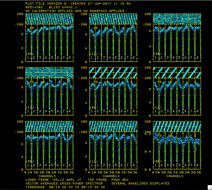
Plot of amplitudes (bottom) and phases (top) for source 0851+202.
Now lets take a look at the fringe finders by running VLBACRPL. VLBACRPL runs POSSM and displays the spectrum of each baseline (to Fort Davis which is antenna 2), with the amplitude on the bottom and the phases on the top.
- default vlbacrpl
- getn 1
- stokes 'half'
- refant 2
- gainuse 0
- solint -1
- dotv 1
- source '0851+202'
- inp
- vlbacrpl
As you can see from Figure 1, 0851+202 has very strong fringes. So we will use it as the calibrator to set the instrumental delays. Also look at your terminal for instructions on how to control POSSM:
POSSM1: Waiting 30 seconds:
POSSM1:    Hit TV button A to pause indefinitely.  Hit button
POSSM1:    B or C to continue sooner, button D to stop plotting
So hit A if you want to look at a plot longer than the 30 seconds, B or C to go to the next plot, D to exit.
You can look at the antennas through AIPS to find a nice reference antenna (refant; here as antenna 2) by running "go prtan".
Determine Delay Corrections
Find and remove instrumental delay by running VLBAPCOR.
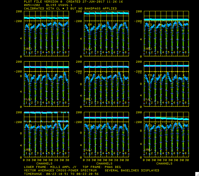
Plots for source 0851+202 which show the amplitude (bottom panel) and corrected phases (top panel), for each IF in both polarizations.
- default vlbapcor
- getn 1
- calsour '0851+202' '
- timer 0 19 26 33 0 19 36 38 ➜ scan with good fringes on all telescopes we found in POSSM plots.
- refant 2 ➜ choose reference antenna from in the middle of array, antenna 2 or FD (Fort Davis, TX) is a good choice.
- gainu 0 ➜ apply highest CL table.
- inp
- vlbapcor
(Note that the second quote sign ' after the source name causes all other values of CALSOUR to be blank.) At this point you should check on the calibration:
- VLBAPCOR runs PCCOR which used the pulse cals to correct the intrumental phases and then runs CLCAL to apply the solutions to the CL (calbration table). The output from VLBAPCOR will look something like this:
AIPS 1: 'RUN PCCOR'
PCCOR1: Task PCCOR  (release of 31DEC17) begins
PCCOR1: Writing to SN table   2
PCCOR1: Appears to have ended successfully
PCCOR1: localhos 31DEC17 TST: Cpu=      0.9  Real=      2  IO=        93
AIPS 1: Resumes
AIPS 1: 'RUN CLCAL'
CLCAL1: Task CLCAL  (release of 31DEC17) begins
CLCAL1: Using interpolation mode SELF
CLCAL1: Copied CL file from vol/cno/vers  1  183   2 to  1  183   3
CLCAL1: CALSEL: Making room for new CL data by
CLCAL1: Deleting CL table no.    3
CLCAL1: Processing SN table    2
CLCAL1: SNMRG: Merging SN table
CLCAL1: SNMRG: Write    2974 merged records from    2974 input records
CLCAL1: SN2CL: Applying SN tables to CL table   2, writing CL table  3
CLCAL1: Appears to have ended successfully
CLCAL1: localhos 31DEC17 TST: Cpu=      0.3  Real=      1  IO=       138
AIPS 1: Resumes
AIPS 1: 'SN #2 CONTAINS PCAL INSTR. PHASE CORRECTIONS'
AIPS 1: 'CL #3 ADDS INSTR. PHASE CORRECTIONS'
Again, it is a good idea to make note of the last two lines that tell you which tables contain which corrections. Most VLBAUTIL calibration scripts produce such messages.
- check solutions in POSSM, the jumps in phase between the IFs should be gone. The phases may also be flattened.
- tget possm ➜ to "get" all the inputs from the last run (it was run when we ran the procedure VLBACRPL).
- gainu 3
- inp
- go
As you can see from Figure 2, the phases for 0851+202 have been flattened and the phase jumps between the IFs are gone. For other sources farther away in time the phases may be different from 0 but there will still be no phase jumps.
Create BP Table and Calibrate Bandpass Shape
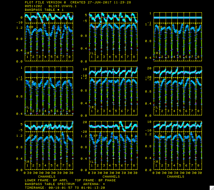
Plot of bandpass for source '0851+202' .
Calibrate bandpass shape with VLBABPSS.
- default vlbabpss
- getn 1
- calsour '0851+202' ' ➜ use a strong source as the bandpass calibrator.
- refant 2
- inp
- vlbabpss
VLBABPSS will create a bandpass (BP) table:
AIPS 1: 'BP #1 BANDPASS TABLE'
Now check the bandpass solutions with POSSM.
- tget possm
- baseline=0
- aparm=0
- aparm(8)=2
- aparm(9)=1
- bpver=1; doband=1
- go
Figure 3 shows the plots generated by POSSM. The solutions should look like a reasonable fit of the bandpass shape.
Apply Amplitude Corrections
Perform amplitude calibration by running VLBAAMP.
- default vlbaamp
- getn 1
- inp
- vlbaamp
Again, the procedure should finish with the following lines:
AIPS 1: 'SN #3 CONTAINS SAMPLER CORRECTIONS'
AIPS 1: 'SN #4 CONTAINS GAIN CORRECTIONS'
AIPS 1: 'CL #4 ADDS SAMPLER CORRECTIONS'
AIPS 1: 'CL #5 ADDS GAIN CORRECTIONS'
which should be noted.
Examine Amplitude Calibration
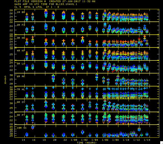
Plot of amplitude gains vs. time with the different colors representing the different IF polarizations.
Examine amplitude calibration by running SNPLT.
- default snplt
- getn 1
- dotv 1
- inext 'cl'
- invers 0
- opty 'amp' ➜ Plot amplitudes.
- nplots 10
- opco 'alsi' ➜ Plot all IFs and Stokes.
- do3col 1 ➜ Use 3-color symbols.
- inp
- tvin ➜ tvinitialize clears the tv before plotting. Otherwise you will get a mess as the table is plotted over the bandpass plot from before.
- go
Figure 4 shows that the amplitude gains change over time as the sources rise and set, with higher gains at lower elevations. The different IFs and polarizations (RR and LL in this case) are shown as different colors.
Correct Phases for Parallactic Angles
Correct phases for parallactic angle effects with VLBAPANG.
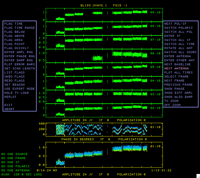
EDITR display showing all the baselines to antenna 10 for 2200+420. You can see for all the baselines the amplitude is low for the first scan and for baseline 01-10 the phases for this scan look like noise. We want to flag this data.
- default vlbapang
- getn 1
- inp
- vlbapang
AIPS 1: 'CL #6 ADDS PARALLACTIC ANGLE CORRECTIONS'
Manually Edit Data
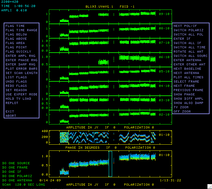
To flag this data we click FLAG TIME RANGE and hit B, and a blue box appears in the 01-10 box on the bottom.
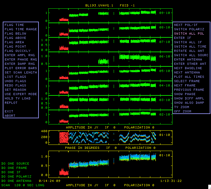
After moving the sides of the box to encompass the data that need to be flagged, hit C and the data are flagged and turn red.
Edit the data using EDITR on each source separately.
- default editr
- getn 1
- docal 1; gainuse 0 ➜ calibrate data with highest CL table.
- crowded 1 ➜ to plot all polarization and IFs on top of each other.
- do3col 1
- doband 1
- bpver 1
- antuse 1 2 3 4 5 6 7 8 9 10 ➜ to plot all the baselines to one antenna at the same time.
Run on one source at a time:
- 0851+202:
- source '0851+202''
- inp
- go
Again look in you terminal window for instructions:
EDITR1: Press buttons A, B, or C to choose an operation
EDITR1: Press button D for on-line help
EDITR plots both amplitudes and phases verses time, so this is a good way to just look at your data. For the inputs we chose, all the polarizations and IFs are plotted on top of each other. The two boxes on the bottom plot these as different colors and show the amplitude and phase for one baseline. The other boxes, where the data are shown in green, are the other baselines to that single antenna. It is especially useful to look at the data this way because problems tend to be antenna based so all the baselines to an antenna will be effected. It you see potentially problematic data (especially high or low amplitudes or with bad phases (note that weak sources will have incoherent phases)), then you should wait to flag until you can see all the baselines to the other antenna in the baseline pair with the bad data. That way you can flag once, telling EDITR to flag all the data for one antenna (this is the default in EDITR, but can be changed). The data for this source looks great. Click "NEXT ANTENNA" found on the menu to the right and press "B" until you have looked at all the baselines on all the antennas for this source. At this point the data has been amplitude calibrated but the source amplitude changes from scan to scan, do you know the reason for this?
Now plot the other sources and inspect.
- 1828+487:
- source '1828+487''
- go
1828+487 also looks pretty good, although there are some ratty amplitudes and phase on the last scan on baselines to antenna 10. We will just leave these for now because the final fringe fit and self-calibration might fix it.
- 2200+420:
- source '2200+420''
- go
As you can see in Figure 5 this source the first scan on the baselines to antenna 10 looks bad. The amplitude is very low and the phases are noise. To flag this data click FLAG TIME RANGE and hit B (Figure 6), and a blue box appears in the 01-10 box on the bottom. By hitting A and moving the cursor move the sides of the box to encompass the data which needs to be flagged; then hit C. The data will be flagged on all the baselines to the antenna and will turn white in the lower colored parts and red in the upper comparison parts of the display (Figure 7).
Fringe Fit the Data
Perform a global fringe fit with FRING. The following steps through imaging are not strictly necessary since we will have to redo them once the geodetic calibration is done, but they are an excellent way to check that the calibration up to this point is correct.
- default fring
- getn 1
- calsour '0851+202', '1828+487', '2200+420' ➜ do a global fringe fit on all sources.
- refant 2
- search 2 9 5 4 1 3 7 8 ➜ list of antennas to search if a solution is hard to find.
- solint 0.25
- doband 1
- bpver 1
- aparm(6) 2 ➜ print some information on solutions.
- aparm(9) 1 ➜ do exhaustive baseline search.
- docal 1; gainu 0
- inp
- go
You should look at the number of good and failed solutions:
FRING1: Found    97646 good solutions
FRING1: Failed on     1042 solutions
FRING1: Adjusting solutions to a common reference antenna
You should get something similar, but not necessarily exactly the same numbers of good and failed solutions. A small percentage of failed solutions are fine at this point. FRING will have created SN table number 5.
Since we did not use a source model, FRING assumes that the calibration source is a point source at the phase center. None of these sources are point sources. Therefore the corrections FRING finds will not correct the data perfectly and, once we apply all the calibration, it will be necessary to do self-calibration with source models to get the best images. Also note that I said "at the phase center" so, no matter what the the true position of your target, this fringe fit will move the brightest spot of the source to the phase center (the position of the target in the correlation).
Apply FRING solutions
Note that the previous step and this step can be done in the single procedure VLBAFRNG. It is broken up here just to show both the steps explicitly, but also because running the tasks individually allows for more control. Here the global fringe fit which was done in the last step is interpolated and applied to the all the calibration that has gone before with CLCAL.
- default clcal
- getn 1
- gainv 6 ➜ CL table with all the calibration.
- gainu 7 ➜ CL table to write next step of calibration in.
- snver 5 ➜ global fringe fit solutions from FRING
- interpol 'SELF' ➜ use 2PT interpolation.
- refant 2
- sour '0851+202', '1828+487', '2200+420' ➜ sources to which to apply calibration.
- calsour sour ➜ set calibrator sources to the same sources in parameter sources
- inp
- go
So SN table #5 will be applied to CL table #6 and create CL table #7 which now includes all the calibration.
Backing up Your Calibration
We will want to save the calibration up to this point with TASAV. TASAV makes a new file with all your calibration tables. This is very useful because it contains everything you need to recalibrate your data in a very compact and portable form. It is also a good idea to do this before you do anything you are unsure about or will change important tables (AN, SU) in ways that are hard to change back.
- default tasav
- getn 1
- outdisk 1
- inp
- go
Lets look at our catalog again:
- uc
You should get something that look similar to:
AIPS 1: Catalog on disk  1
AIPS 1:   Cat  Usid Mapname      Class   Seq  Pt    Last access     Stat
AIPS 1:     1   193 BL193BG     .UVAVG .    1 UV 01-JUL-17 14:28:24
AIPS 1:     2   193 BL193BG     .TASAV .    1 UV 27-JUN-17 11:52:14
Note that you now have a second catalog entry which TASAV automatically named BL193BG.TASAV.1. This uv data file has 1 visibility and all the tables attached to BL193BG.UVDATA.1. Lets look at the TASAVed file.:
- getn 2
- imh
You should get something that looks like:
AIPS 1: Image=MULTI     (UV)         Filename=BL193BG     .TASAV .   1
AIPS 1: Telescope=VLBA               Receiver=VLBA
AIPS 1: Observer=BL193BG             User #=  193
AIPS 1: Observ. date=16-JUN-2016     Map date=27-JUN-2017
AIPS 1: # visibilities         1     Sort order  TB
AIPS 1: Rand axes: UU-L-SIN  VV-L-SIN  WW-L-SIN  TIME1  SUBARRAY
AIPS 1:            SOURCE  REMOVED  INTTIM  GATEID  CORR-ID  ANTENNA1
AIPS 1:            ANTENNA2
AIPS 1: ----------------------------------------------------------------
AIPS 1: Type    Pixels   Coord value     at Pixel     Coord incr   Rotat
AIPS 1: COMPLEX      3   1.0000000E+00       1.00  1.0000000E+00    0.00
AIPS 1: STOKES       2  -1.0000000E+00       1.00 -1.0000000E+00    0.00
AIPS 1: FREQ        32   1.5240375E+10      17.00  1.0000000E+06    0.00
AIPS 1: IF           8   1.0000000E+00       1.00  1.0000000E+00    0.00
AIPS 1: RA           1    00 00 00.000       1.00       3600.000    0.00
AIPS 1: DEC          1    00 00 00.000       1.00       3600.000    0.00
AIPS 1: ----------------------------------------------------------------
AIPS 1: Coordinate equinox 2000.00
AIPS 1: Maximum version number of extension files of type HI is   1
AIPS 1: Maximum version number of extension files of type AT is   1
AIPS 1: Maximum version number of extension files of type CT is   1
AIPS 1: Maximum version number of extension files of type FQ is   1
AIPS 1: Maximum version number of extension files of type AN is   1
AIPS 1: Maximum version number of extension files of type CL is   7
AIPS 1: Maximum version number of extension files of type CQ is   1
AIPS 1: Maximum version number of extension files of type GC is   1
AIPS 1: Maximum version number of extension files of type IM is   1
AIPS 1: Maximum version number of extension files of type MC is   1
AIPS 1: Maximum version number of extension files of type PC is   1
AIPS 1: Maximum version number of extension files of type SU is   1
AIPS 1: Maximum version number of extension files of type TY is   1
AIPS 1: Maximum version number of extension files of type WX is   1
AIPS 1: Maximum version number of extension files of type SN is   5
AIPS 1: Maximum version number of extension files of type BP is   1
AIPS 1: Maximum version number of extension files of type FG is   1
Note that there is 1 visibility but 7 calibration (CL) tables and 5 solution (SN) tables. As well as numerous other tables with information about you data (history (HI), frequency (FQ), antenna (AN), system temperature (TY), bandpass (BP), flag (FG)...).
Apply Calibration and SPLIT the Data
Apply calibration and make single source data sets with SPLIT. I like to work with single source files, it's less confusing, especially when self-caling and imaging.
- default split
- getn 1
- freqid 0
- docal 1; gainu 7 ➜ apply calibration; from CL#7.
- sour '0851+202', '1828+487', '2200+420'
- doband 1; bpver 1
- aparm 2 0 0 0 1 1 ➜ aparm(1)=2 tells SPLIT to average all the channels in each IF, reducing the size of the data significantly.
- inp
- go
This will produce three files named sourcename.SPLIT.1, again type uc to look at the catalog.
AIPS 1: Catalog on disk  1
AIPS 1:   Cat  Usid Mapname      Class   Seq  Pt    Last access     Stat
AIPS 1:     1   193 BL193BG     .UVAVG .    1 UV 01-JUL-17 14:28:24
AIPS 1:     2   193 BL193BG     .TASAV .    1 UV 03-JUL-17 15:01:55
AIPS 1:     3   193 2200+420    .SPLIT .    1 UV 03-JUL-17 15:12:12
AIPS 1:     4   193 0851+202    .SPLIT .    1 UV 03-JUL-17 15:14:41
AIPS 1:     5   193 1828+487    .SPLIT .    1 UV 03-JUL-17 15:15:29
OPTIONAL: Getting the Calibrated Data
THIS STEP IS OPTIONAL: If everything went well in the above steps there is no need to get the calibrated data.
However If something went wrong with the calibration or if you want to start with the imaging and self-calibration then download the following files and put them in your $FITS area:
- 0851+202.SPLIT.1 (6.3 MB): Calibrated data for source 0851+202.
- 1828+487.SPLIT.1 (7.8 MB): Calibrated data for source 1828+487.
- 2200+420.SPLIT.1 (6.8 MB): Calibrated data for source 2200+420.
Then load the data with FITLD:
- default fitld
- datain 'MYAIP:0851+202.SPLIT.1
- outdisk 1
- inp
- go
and repeat for 1828+487.SPLIT.1 and 2200+420.SPLIT.1.
Note that these data do not include self-calibration but does include flagging.
Flagging 1828+487
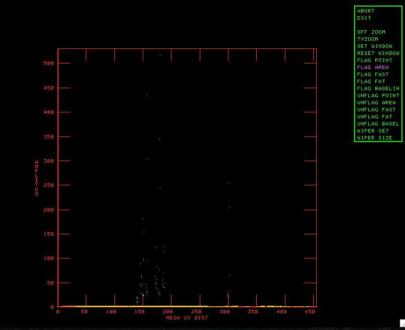
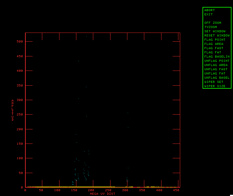
WIPER plot of amplitude vs UV distance.
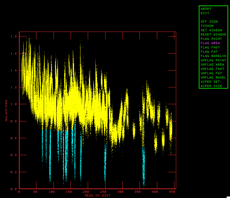
WIPER plot with high amp points flagged (in blue).
WIPER plot with low amp points flagged (in blue).
Let's do some more flagging before we get into imaging. A nice graphical flagging task that is especially useful after SPLITing is WIPER. WIPER defaults to plot amplitude vs uv distance:
- default wiper
- getn 5
- imsi 512
- inp
- go
Ick! Look at those high points (Figure 8). Flag those by clicking on FLAG AREA, setting a box hitting the "A" key then hitting the "C" key when done, the flaged points will turn blue as in Figure 9. Now click EXIT and hit "A". Immediately type "go" to run WIPER again. This is more like it (Figure 10), but there are some low points, flag those with FLAG AREA but don't be too overzealous.
Now you have 2 flag (FG) tables attached to the data, one for each run of WIPER. FG table 2 has all the flags in it.
Imaging and Self-Cal of 1828+487
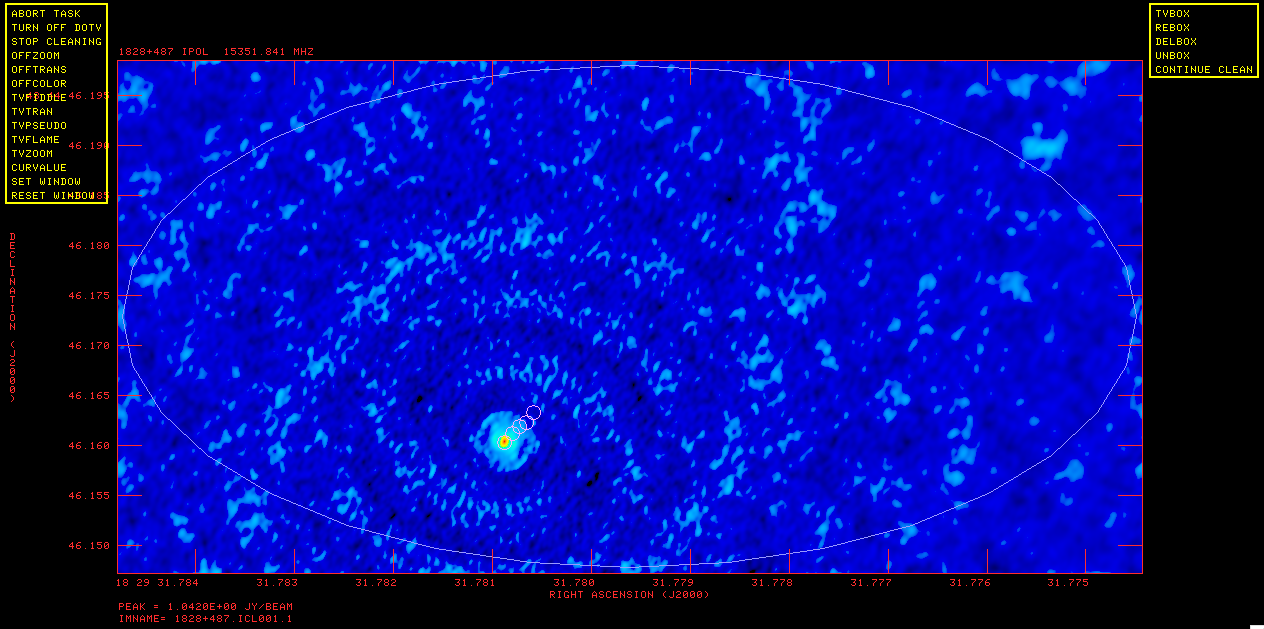
Dirty map of 1828+487.
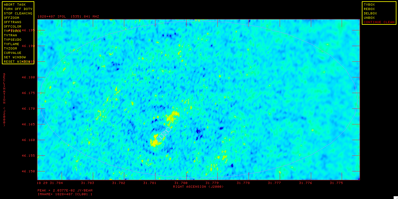
Residual map of 1828+487.
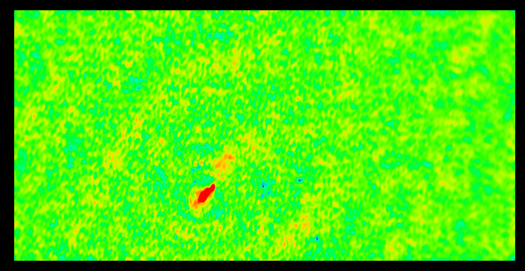
Image of 1828+487 after first run of IMAGR.
Lets start by imaging 1828+487 with IMAGR. Either use the clean box files provided (make sure they are in the $MYAIP directory) or do interactive boxing. Using the supplied box file is easier. Also lets make sure that dowait=1 by typing:
- dowait=1
Note that I came up with the parameters below especially the IMSIZE, ROBUST, RASH and DECSH by imaging and experimenting. Task SETFC can be used to recommend CELLSIZE and IMSIZE if you specify a desired field of view. The shifts were chosen, for this source only, to center the object including its jet within the image. It is recommended that you use the supplied box files. They reflect both the very obvious emission in the field and additional information from the MOJAVE project.
- default imagr
- getn 5
- cell 0.0001; imsi 1024 512 ➜ cell size of 0.1 mas; image size of 1024x512.
- rash -0.0125 0
- decsh 0.0125 0
- dotv 1
- robust 5 ➜ Do natural weighting. This source has a big diffuse jet, therefore sensitivity and more weight on the short spacings is more important than high resolution.
- niter 5000 ➜ do interactive clean; with 5000 iterations, you will probably "stop cleaning" before hitting 5000 on the first iteration of imaging.
- boxfile 'MYAIP:1828_1.box
- inp
- go
- recat
Hit TVPSEUDO then "B" immediately to get color rather than grey scale. Figure 11 shows the dirty map. If you want to clean interactively, then click CONTINUE CLEAN (and "A"); after a few rounds of cleaning (about 300 clean components which the messages from IMAGR tell you) the residuals will look like Figure 12. You can see in Figure 12 there is not much else to clean inside the clean boxes although there is some flux outside the clean boxes. This isn't significant enough to box at this point, so click STOP CLEANING ("A"). IMAGR will return the cleaned map, Figure 13, as you can see there are artifacts in the map.
Once IMAGR is done you run RECAT, which compresses the catalog so there are no empty spaces. This is not strictly necessary, but to follow this tutorial and have the GETN work, we have to be sure that the catalog numbers are consistent. Now do a mcat (mc for short) to look at the maps in your catalog:
- mc
AIPS 1: Catalog on disk  1
AIPS 1:   Cat  Usid Mapname      Class   Seq  Pt    Last access     Stat
AIPS 1:     6   195 1828+487    .IBM001.    1 MA 04-JUL-17 10:33:14
AIPS 1:     7   195 1828+487    .ICL001.    1 MA 04-JUL-17 10:33:14
Note that you have made two files, a "dirty beam" (the IBM001 file) and a cleaned map (ICL001).
To look at the image use TVLOD (getn 6; tvin; tvlo). Use TVPSEUDO to put it into color (tvps). You can use your mouse to manipulate the colors; again look at your terminal for instructions. Hit "D" once it looks the way you want. Figure 11 shows the image with the stretch set so the noise level is obvious.
Lets measure the rms in the cleaned image with IMEAN:
- default imean
- getn 7
- go
The rms for this image using IMEAN's histogram fitting in units of Janskys/beam is:
IMEAN1: Mean=-1.0708E-04 Rms= 2.2822E-03 **** from histogram
IMEAN also gives you other statistics about the image such as the maximum and total flux.
So the image isn't the best, the noise is much higher than desirable, and there are hints of lower level structure but they are not much higher than the noise. So it looks like self-calibration would be beneficial. At some level self-cal is an art rather than a science, and there are various different philosophies concerning how to best do self-cal. I tend to be conservative, partially because VLBA data has fewer baselines and therefore it is easier to go off in a bad direction with the self-cal. However, these are fairly strong sources so it will be harder to make big mistakes in the self-calibration. Self-cal is done by the task CALIB. Generally phase-only self-cal should be done first, then amplitude and phase. Also we will be using clean component models (i.e., the image we just made) for the self-calibration.
- default calib
- getn 5
- get2n 7 ➜ use clean components from this map as a model for the self-cal
- refant 2
- solint 1 ➜ 1 minute solution interval
- solty 'l1r' ➜ type of method for solution (see EXPLAIN CALIB for more details)
- solmo 'P' ➜ solve for phases only
- inp
- go
- recat
You will get messages that look like this:
CALIB1: Task CALIB  (release of 31DEC17) begins
CALIB1: Using 1828+487 . SPLIT . 1  Disk= 1 Usid= 195
CALIB1: L1 Solution type
CALIB1: UVGET: Using flag table version   2 to edit data
CALIB1: Create 1828+487    .CALIB .   1 (UV)  on disk  1  cno    8
CALIB1: Selecting and editing the data
CALIB1: Using Clean Component self-cal source model
CALIB1: FACSET: 1.375524 Jy found from 209 components
CALIB1: Divide data by model - first compute model by summing
CALIB1: QINIT: did a GET  of      5120 Kwords, OFF          5241849
CALIB1: ALGMEM field    1 Ipol gridded model subtraction chns    1-    8
CALIB1: ALGMEM: at visibility number           1
CALIB1: ALGMEM:  1024 - 0 cells, with       23349 Pts
CALIB1: Field    1 used     209 CCs
CALIB1: Determining solutions using full vector averaging
CALIB1: Writing SN table    1
CALIB1: Found         7380 good solutions
CALIB1:                  7 solutions had no data
CALIB1: Average closure rms =  0.03470 +-  0.00913
CALIB1: Fraction of times having data >  2.5 rms from solution
CALIB1: 0.24661 of the times had  2 -  4 percent outside  2.5 times rms
CALIB1: 0.09842 of the times had  4 -  6 percent outside  2.5 times rms
CALIB1: 0.06674 of the times had  6 -  8 percent outside  2.5 times rms
CALIB1: 0.08258 of the times had  8 - 10 percent outside  2.5 times rms
CALIB1: 0.07579 of the times had 10 - 12 percent outside  2.5 times rms
CALIB1: 0.06900 of the times had 12 - 14 percent outside  2.5 times rms
CALIB1: 0.04186 of the times had 14 - 16 percent outside  2.5 times rms
CALIB1: 0.02602 of the times had 16 - 18 percent outside  2.5 times rms
CALIB1: 0.01810 of the times had 18 - 20 percent outside  2.5 times rms
CALIB1: 0.01131 of the times had 22 - 24 percent outside  2.5 times rms
CALIB1: 0.00113 of the times had 26 - 28 percent outside  2.5 times rms
CALIB1: Applying solutions to data
CALIB1:            Previously flagged   Flagged by gain         Kept
CALIB1: Partially                  341                   0       341
CALIB1: Fully                        0                   0     23008
CALIB1: Copied WX file from vol/cno/vers  1    5   1 to  1    8   1
CALIB1: Copied AN file from vol/cno/vers  1    5   1 to  1    8   1
CALIB1: Copied FG file from vol/cno/vers  1    5   1 to  1    8   1
CALIB1: Copied FG file from vol/cno/vers  1    5   2 to  1    8   2
CALIB1: Appears to have ended successfully
There are several things you should note in these messages:
- CALIB creates a new UV file called 1828+487.CALIB.1 at catalog number 8
- CALIB also writes an SN table attached to the input data file
- CALIB found 7380 good solutions, 7 had no data and did not fail on any
- CALIB didn't flag any new data. Since this is such a strong source CALIB probably will not flag any of the data. However for weaker sources this is a concern, a bad model and a weak source could mean that some portion of your input data is flagged by CALIB, meaning you can take your imaging to strange places if you are not careful.
Now we image the corrected data. We can either use the file that CALIB created or the original file applying the SN table that CALIB attached to it. Just for brevity we will use the file CALIB created:
- tget imagr
- getn 8
- boxfi 'MYAIP:1828_2.box
- inp
- go; recat
After about 1500 clean components the map looks sufficiently clean. While doing the interactive clean the residuals did look better than in the first imaging but lets do IMEAN again (tget imean; getn 10; go) to confirm the rms is getting lower. The noise is now ~1.3E-03 Jy/beam, so a significant drop, but we can probably still do better. So more self-cal, with a shorter solution interval:
- tget calib
- get2n 10
- solint 0.5
- go; recat
Now we have:
CALIB1: Writing SN table    2
CALIB1: Found        14749 good solutions
CALIB1:                 12 solutions had no data
Image again:
- tget imagr
- getn 11
- go; recat
IMEAN again:
- tget imean
- getn 13
- go
Now the rms is about 1.1E-3 Jy/beam, so a little lower than last time but a much smaller drop. Lets try a much smaller solution interval.
- tget calib
- get2n 13
- solint 0.1
- go; recat
Now we have:
CALIB1: Writing SN table    3
CALIB1: Found        53090 good solutions
CALIB1: Failed on       72 solutions
CALIB1:                 92 solutions had no data
So CALIB failed on a tiny fraction of solutions and flagged a tiny fraction of the data. This is OK, it just means that with this solution interval we are on the edge of not having enough sensitivity to get good solutions.
Image again:
- tget imagr
- getn 14
- boxfi 'MYAIP:1828_3.box
- go; recat
IMEAN again:
- tget imean
- getn 16
- go
Now the rms is about 8.8E-4 Jy/beam, another significant drop, either the low solint or the extra box is making things better, probably both. So lets do one more phase only self cal with this solution interval before going to amplitude and phase.
- tget calib
- get2n 16
- go; recat
Now we have:
CALIB1: Writing SN table    4
CALIB1: Found        53093 good solutions
CALIB1: Failed on       69 solutions
CALIB1:                 92 solutions had no data
Note that it failed on fewer solutions that last time, another indication that the additional box added to the cleaning allowed for model that fit the data better.
Image again:
- tget imagr
- getn 17
- go; recat
IMEAN again:
- tget imean
- getn 19
- go
Now the rms is about 8.5E-4 Jy/beam, so another small drop.
Lets move to amplitude self cal. You might have noticed that for the runs of CALIB we went back to the original data rather than the self-caled data. This is one of those philosophies of self-cal I mentioned earlier, you could have used the the output file from CALIB and done smaller increments of self-cal, I prefer to go back to the original data and just improve the model. I do this because here is less chance of getting an incorrect model stuck in the data with this method. However once we move to amplitude self-cal we want to use the data with the best calibrated phases so we will start with the last file out of CALIB.
- tget calib
- getn 17
- get2n 19
- solint 1
- solmo 'a&p'
- go; recat
Now we have:
CALIB1: Writing SN table    1
CALIB1: RPOL, IF= 1 The average gain over these antennas is  9.897E-01
CALIB1: RPOL, IF= 2 The average gain over these antennas is  1.001E+00
CALIB1: RPOL, IF= 3 The average gain over these antennas is  1.007E+00
CALIB1: RPOL, IF= 4 The average gain over these antennas is  1.008E+00
CALIB1: RPOL, IF= 5 The average gain over these antennas is  1.007E+00
CALIB1: RPOL, IF= 6 The average gain over these antennas is  1.003E+00
CALIB1: RPOL, IF= 7 The average gain over these antennas is  1.012E+00
CALIB1: RPOL, IF= 8 The average gain over these antennas is  1.003E+00
CALIB1: LPOL, IF= 1 The average gain over these antennas is  1.002E+00
CALIB1: LPOL, IF= 2 The average gain over these antennas is  1.003E+00
CALIB1: LPOL, IF= 3 The average gain over these antennas is  1.012E+00
CALIB1: LPOL, IF= 4 The average gain over these antennas is  1.009E+00
CALIB1: LPOL, IF= 5 The average gain over these antennas is  1.000E+00
CALIB1: LPOL, IF= 6 The average gain over these antennas is  1.010E+00
CALIB1: LPOL, IF= 7 The average gain over these antennas is  1.020E+00
CALIB1: LPOL, IF= 8 The average gain over these antennas is  1.016E+00
CALIB1: Found         7380 good solutions
CALIB1:                  7 solutions had no data
Similar messages to the phase only except it now tells you how it is adjusting the amplitudes in each IF/polarization.
Image again:
- tget imagr
- getn 20
- boxfi 'MYAIP:1828_4.box
- go; recat
You may have noticed that I am avoiding boxed the bright stuff around the core, because it is around the brightest thing in the map I am worried it is just sidelobes that have not been cleaned properly, at this point I am contemplating boxing it. Also next time we run IMAGR I will increase the number of iterations, 5000 seems like barely enough.
IMEAN again:
- tget imean
- getn 22
- go
Now the rms is about 2.8E-4 Jy/beam, a big drop.
Since we have a lot more structures in the model we should do more self-cal.
- tget calib
- get2n 22
- go; recat
Now we have:
CALIB1: Writing SN table    2
CALIB1: RPOL, IF= 1 The average gain over these antennas is  9.909E-01
CALIB1: RPOL, IF= 2 The average gain over these antennas is  1.003E+00
CALIB1: RPOL, IF= 3 The average gain over these antennas is  1.008E+00
CALIB1: RPOL, IF= 4 The average gain over these antennas is  1.009E+00
CALIB1: RPOL, IF= 5 The average gain over these antennas is  1.008E+00
CALIB1: RPOL, IF= 6 The average gain over these antennas is  1.004E+00
CALIB1: RPOL, IF= 7 The average gain over these antennas is  1.013E+00
CALIB1: RPOL, IF= 8 The average gain over these antennas is  1.004E+00
CALIB1: LPOL, IF= 1 The average gain over these antennas is  1.003E+00
CALIB1: LPOL, IF= 2 The average gain over these antennas is  1.004E+00
CALIB1: LPOL, IF= 3 The average gain over these antennas is  1.013E+00
CALIB1: LPOL, IF= 4 The average gain over these antennas is  1.010E+00
CALIB1: LPOL, IF= 5 The average gain over these antennas is  1.001E+00
CALIB1: LPOL, IF= 6 The average gain over these antennas is  1.011E+00
CALIB1: LPOL, IF= 7 The average gain over these antennas is  1.021E+00
CALIB1: LPOL, IF= 8 The average gain over these antennas is  1.017E+00
CALIB1: Found         7380 good solutions
CALIB1:                  7 solutions had no data
Image again:
- tget imagr
- getn 23
- niter 10000
- go; recat
IMEAN again:
- tget imean
- getn 25
- go
Now the rms is about 1.7E-4 Jy/beam, a big drop, CALIB liked the new model with all that extra part of the jet boxed, which is a good sign. Also in the residuals the emission around the core is much fainter, so it looks like it was good we did not box it. More self-cal can be done, but a majority of the improvement has been accomplished.
Making a Contour Map
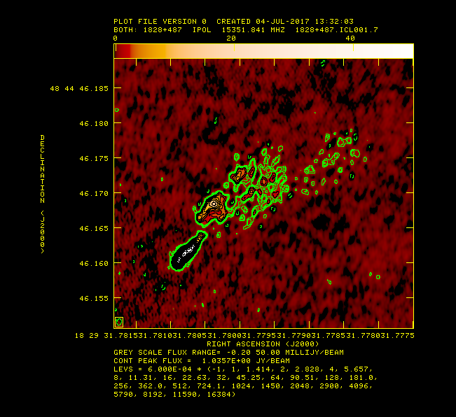
Contour map of 1828+487 after self calibration.
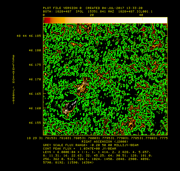
Countour map of 1828+487 before self calibration.
What is the best way to look at the images, particularly with all this low level structure? One of the best ways is with a contour map. We will use KNTR to make such a map. I came up with the following parameters after some experimentation.
- default kntr
- getn 25
- dovect -1
- dotv 1
- ofmfile 'ryphlame'
- clev 5e-4
- blc 295 35
- trc 721 419
- pixra -0.0002 0.05
- functy 'l2'
- levs(1)=-1
- for i=2 to 30; levs(i)=2**((i-2)/2.); end
- inp
- tvin; go
- recat
Note that I used verb TVWIN to set blc and trc (bottom left corner and top right corner of the image to plot). Also I am using a for loop to set the contour levels in a logarithmic fashion. I have set the contour level multiplier (clev) and the pixel range (pixra) so that we can see some of the noise. I am also using an ofm file for the background. To see all the ofm files that come with AIPS type "OFMDIR"; ofmfile 'rainbow' is closest to tvpseudo. Figure 14 shows what the figure looks like on the TV.
Just for fun run KNTR with the same inputs on the image of 1828+487 before all the self-calibration. Figure 15 shows what you get, the vast improvement made by the self calibration is obvious.
To make a hard copy of this figure set DOTV to -1 and run KNTR, KNTR will produce a PL (plot) table. Then run LWPLA to make a postscript of that PL table.
- default lwpla
- getn 25; outfi 'MYAIP:1828+487.ps
- go
This produces a postscript file in the $MYAIP directory.
Create More Images
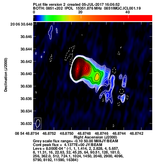
Contour map of 0851+202 (OJ287) after self calibration. This is a version of the image that uses LWPLA to make a hardcopy after KNTR.
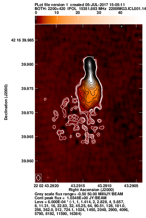
Contour map of 2200+420 (BL Lac) after self calibration. This is a version of the image that uses LWPLA to make a hardcopy after KNTR.
Image 2200+420 and/or 0851+202 with IMAGR.
- tget imagr
- getn 3 or 4
- rash 0
- decsh 0
- imsi 512
- inp
- go
You can follow similar steps with WIPER and self-calibration on these sources.
Doing All the Calibration (Except the Self-Calibration) With a Pipeline
Inside AIPS there is a procedure VLBARUN which will do all the calibration steps above except for the interactive flagging and self-calibration. VLBARUN uses the VLBAUTIL procedures to calibrate the data with little intervention. In the 31DEC19 release of AIPS, it also offers the option of adding known flags through a text file and doing auto-editing via task RFLAG.
Just to be safe type RESTORE 0, which will remove all the procedures from the AIPS "memory". It is also best if VLBARUN is run in a pristine environment, to do this restart AIPS (just type "restart" from inside AIPS) and use a different AIPS number. Then load the two sets of procedures:
- run vlbautil
- run vlbarun
Next set up the VLBARUN inputs, here I assume you want VLBARUN load the data, but VLBARUN can also be be run on data that is already loaded :
- default vlbarun
- datain 'FITS:bl193bg_3sour_avg.fits
- outname 'bl195bg'
- outdisk 1
- indisk outdisk
- opty 'cont'
- clint 0.25
- calsour '0851+202' '1828+487' '2200+420'
- solint 0.25
- factor 2
- doflag 1
- doplot 1
- outfi some directory below which to put plots and .html file for examination such as 'PWD:' or '/path/to/dir
- outtext your@email.edu
- vlbarun
Since I set doplot=1 and outfile the procedure will produce diagnostic plots putting them in a dated directory below the directory set in outfile and write an html page to allow you to examine the plots easily. The message file is also stored in this directory. For a (new) example of the output for this data see vlbarun.html, the main difference is that VLBARUN ran VLBAEOPS, which we skipped so there is one more CL table. FLAGR was also run so there are not so many bad samples in the UVPLTs of the calibrated data.