VLA CASA Pipeline-CASA4.5.3: Difference between revisions
| (299 intermediate revisions by 3 users not shown) | |||
| Line 1: | Line 1: | ||
'''This guide is designed for CASA 4.5.3''' | |||
== Introduction == | == Introduction == | ||
The VLA calibration pipeline is described on the [https://science.nrao.edu/facilities/vla/data-processing/pipeline VLA pipeline webpage.] | When VLA observations are complete, the raw data need to be calibrated for scientific applications. This is achieved through various steps, as explained in the [https://casaguides.nrao.edu/index.php/Karl_G._Jansky_VLA_Tutorials VLA CASA tutorials.] The different calibration procedures are also bundled in a general VLA calibration pipeline that is described on the [https://science.nrao.edu/facilities/vla/data-processing/pipeline VLA pipeline webpage.] At NRAO, the pipeline is now executed on every science scheduling block (SB) that the VLA observes successfully. At this time, scientific target imaging is not part of the VLA pipeline. Manual imaging steps, however, are explained in the VLA CASA tutorials. | ||
There are currently two maintained versions of the VLA pipeline: A calibration pipeline integrated in CASA, and an external, scripted pipeline. This VLA pipeline CASA tutorial guides through the version that is integrated in CASA. It is developed along with the ALMA pipeline and aims to produce similar output (documentation for ALMA is available through the [https://almascience.nrao.edu/documents-and-tools almascience.org portal/Documents & Tools]). Details on the scripted pipeline can be found on the [https://science.nrao.edu/facilities/vla/data-processing/pipeline/scripted-pipeline VLA scripted pipeline webpage.] | |||
The VLA pipeline has been developed to | The VLA pipeline has been developed to work work for all 1-50 GHz VLA data without manual intervention. All calibration steps are applied to all data; this implies that simplicity and robustness currently have priority over speed. Pipeline runs can take anywhere from a few hours to several days, with a typical VLA scheduling block (SB) being processed within the time span of about a day. | ||
The pipeline was introduced in May 2012 and usually works well for all data taken thereafter. It may not work without modifications for data taken earlier and for such observations we recommend adjusting the scripted pipeline or to perform the calibration steps manually. | |||
<!-- | <!-- | ||
| Line 50: | Line 52: | ||
== Pipeline Requirements == | == Pipeline Requirements == | ||
The VLA pipeline has been developed for Stokes I | The VLA pipeline has been developed for Stokes I continuum data with a range of spectral windows (spws) that are typically 128MHz wide. Nevertheless, it usually also performs well on other setups, although it is currently not tailored for non-Stokes I continuum cases. In the future, we will provide a reprocessing interface that allows the user to adapt the pipeline to the specifics of their observations including spectral line, and polarization. In the following we will also explain how to adapt the pipeline, e.g., for spectral line setups. | ||
The pipeline relies on the correct setting of the scan intents. We therefore recommend that every observer ensures that the scan intents are correctly specified in the Observation Preparation Tool (OPT) during the preparation of the observing script (see [https://science.nrao.edu/facilities/vla/docs/manuals/opt OPT manual] for details). In particular, the pipeline requires the intents CALIBRATE_FLUX to mark flux density calibration scans (toward one of the standard VLA calibrators 3C48, 3C138, 3C147, or 3C286), CALIBRATE_AMPLI and CALIBRATE_PHASE for the temporal complex gain/phase calibration, and CALIBRATE_BANDPASS for the scan that is used to obtain the bandpass calibration (only the first instance of CALIBRATE_BANDPASS is used). CALIBRATE_DELAY marks the delay calibrator scan. If CALIBRATE_DELAY is not set, delay calibration will use the scans with a CALIBRATE_BANDPASS intent. If CALIBRATE_BANDPASS is absent, bandpass calibration (and possibly delay calibration) will use the CALIBRATE_FLUX scan(s). | |||
The pipeline also currently requires a signal-to-noise of >~3 for each spectral window of a calibrator per integration (for each channel of the bandpass). | |||
<!-- | <!-- | ||
| Line 110: | Line 112: | ||
--> | --> | ||
== | == Pipeline Execution == | ||
=== NRAO- | === NRAO-Initiated Automatic Pipeline Runs === | ||
Every schedule block (SB) executed at the VLA will be batch pipeline processed. NRAO | Every science schedule block (SB) executed successfully at the VLA will be batch pipeline processed. NRAO uses a pipeline version that is distributed with CASA and available for general use (see [https://casa.nrao.edu/casa_obtaining.shtml the CASA download page] for all pipeline versions). At NRAO, we will always execute the standard pipeline, which implies that it is optimized for Stokes I continuum processing independent of the actual science goal. A user may therefore decide to re-run the pipeline after making appropriate modifications. | ||
Once an SB | Once an SB has been processed, the PI of the project will receive an email that pipeline calibrated data are available and can be requested via the [https://help.nrao.edu/ NRAO helpdesk]. For ~15 days, the calibrated MeasurementSet (MS) will be stored for download. After that period the calibrated MS is deleted, but the weblog and | ||
calibration and flagging tables are archived. These products may be retrieved and applied to the raw MS (downloaded from the archive) to obtain calibrated visibilities (see the [https://science.nrao.edu/facilities/vla/data-processing/pipeline VLA pipeline webpage] for more details). | |||
The user should inspect the weblog and the calibrated data from the VLA pipeline results carefully. Usually, some additional flagging and reprocessing will be required for better results. Upon request through the [https://help.nrao.edu/ NRAO helpdesk] a member of the staff can perform a detailed quality assessment of the pipeline results based on this weblog. | |||
=== Starting the Pipeline Manually === | === Starting the Pipeline Manually === | ||
The [https://science.nrao.edu/facilities/vla/data-processing/pipeline VLA pipeline webpage] | Pipeline processing can be quite computing intensive. On the [https://casa.nrao.edu/casa_hardware-requirements.shtml CASA Hardware Requirements page] some recommendations for a suitable computing infrastructure are provided. If you would like to use the [https://science.nrao.edu/facilities/vla/docs/manuals/computing-resources/overview NRAO lustre/cluster system], please request an account through the [https://help.nrao.edu/ NRAO helpdesk]. | ||
The [https://science.nrao.edu/facilities/vla/data-processing/pipeline VLA pipeline webpage] provides details on how to execute the VLA pipeline. To start with, a CASA version with integrated pipeline heuristic code is required and can be downloaded from the [https://casa.nrao.edu/casa_obtaining.shtml CASA webpages]. | |||
We also recommend to download the VLA raw data from the [https://archive.nrao.edu/archive/advquery.jsp NRAO archive] in the form of a 'Science Data Model-Binary Data Format' (SDM-BDF), the raw VLA archive data format (although MeasurementSets may also work). | |||
<source lang=" | If you want to run the pipeline for the data that is shown in this guide, search the NRAO archive for the "Archive File ID": 13A-398.sb17165245.eb19476558.56374.213876608796 | ||
To include the pipeline heuristic tasks, start CASA with the ''--pipeline'' option: | |||
<source lang="bash"> | |||
# In a Terminal | # In a Terminal | ||
casa --pipeline | casa --pipeline | ||
</source> | </source> | ||
At NRAO one can start the current default pipeline version via: | |||
<source lang=" | <source lang="bash"> | ||
# In a Terminal | # In a Terminal | ||
casa-pipe | casa-pipe | ||
</source> | </source> | ||
Next, at the CASA prompt, import the VLA pipeline recipes as: | |||
<source lang="python"> | <source lang="python"> | ||
| Line 143: | Line 154: | ||
</source> | </source> | ||
<!-- | |||
(other, specialized recipes may be available as well) | |||
--> | |||
The actual execution of the pipeline on the SDM, in our example ''13A-398.sb17165245.eb19476558.56374.213876608796'', will be initiated like: | |||
<source lang="python"> | |||
# In CASA | |||
hifv.hifv(['13A-398.sb17165245.eb19476558.56374.213876608796']) | |||
</source> | |||
The pipeline will now start processing the data. Depending on the data size and structure, processing times range somewhere between a few hours and several days. | |||
== Pipeline Output == | |||
VLA pipeline output includes: | |||
* An '''MS with calibrated visibilities in the CORRECTED_DATA column''' that can be used for subsequent imaging (in the root directory of the pipeline run). | |||
* '''Calibrator images for all spws''' (files ''oussid*'' in the root directory; see the descriptions of the tasks ''hifv_makeimlist'' and ''hifv_makeimages'' below). | |||
* All '''calibration tables''' and the '''MS.flagversions''' directory that contains various flag backups made at various stages of the pipeline run (root directory). | |||
* A '''weblog''' that is accessible via '''pipelineTIME/html/index.html''', where the TIME stands for the pipeline execution time stamp (multiple pipeline executions will result in multiple weblogs). | |||
* The '''casapyTIME.log''' CASA logger messages (in ''pipelineTIME/html/''). | |||
* '''casa_pipescript.py''' (in ''pipelineTIME/html/''), the script with the actually executed pipeline heuristic sequence and parameter (see below). | |||
* '''casa_commands.log''' (in ''pipelineTIME/html/''), which contains the actual CASA commands that were generated by the pipeline heuristics (see below). | |||
* The '''{{listobs}} output''' is available under ''pipelineTIME/html/sessionSession_default/<MSname>.listobs.txt'' and contains the characteristics of the observations (scans, source fields, spectral setup, antenna positions, and general information). | |||
=== Calibration Tables === | |||
The final calibration tables of the pipeline are (where <SDM> is a placeholder for the SDM name): | |||
<SDM>.ms.hifv_priorcals.s5_3.gc.tbl : Gaincurve | |||
<SDM>.ms.hifv_priorcals.s5_4.opac.tbl : Opacity | |||
<SDM>.ms.hifv_priorcals.s5_5.rq.tbl : Requantizer gains | |||
<SDM>.ms.hifv_priorcals.s5_6.ants.tbl : Antenna position offsets | |||
<SDM>.ms.finaldelay.k : Delay | |||
<SDM>.ms.finalBPcal.b : Bandpass | |||
<SDM>.ms.averagephasegain.g : Temporal Phase offsets | |||
<SDM>.ms.finalampgaincal.g : Flux calibrated Temporal Gains | |||
<SDM>.ms.finalphasegaincal.g : Temporal Phases | |||
=== casa_pipescript.py === | |||
VLA pipeline heuristic tasks start with ''hifv'' for 'heuristics, interferometry, vla'. The pipeline sequence of the pipeline heuristic steps are listed in the 'casa_pipescript.py' that is located in the 'pipelineTIME/html' (where TIME is the timestamp of the execution) directory. For our example, 'casa_pipescript.py' has the following structure: | |||
<pre style="white-space: pre-wrap;"> | |||
__rethrow_casa_exceptions = True | |||
h_init() | |||
try: | |||
hifv_importdata(ocorr_mode='co', vis=['13A-398.sb17165245.eb19476558.56374.213876608796'], createmms='automatic', asis='Receiver CalAtmosphere', overwrite=True) | |||
hifv_hanning(pipelinemode="automatic") | |||
hifv_flagdata(intents='*POINTING*,*FOCUS*,*ATMOSPHERE*,*SIDEBAND_RATIO*, *UNKNOWN*, *SYSTEM_CONFIGURATION*, *UNSPECIFIED#UNSPECIFIED*', flagbackup=False, scan=True, baseband=True, clip=True, autocorr=True, hm_tbuff='1.5int', template=False, online=True, tbuff=0.0, fracspw=0.05, shadow=True, quack=True, edgespw=True) | |||
hifv_vlasetjy(fluxdensity=-1, scalebychan=True, reffreq='1GHz', spix=0) | |||
hifv_priorcals(pipelinemode="automatic") | |||
hifv_testBPdcals(pipelinemode="automatic") | |||
hifv_flagbaddef(pipelinemode="automatic") | |||
hifv_checkflag(pipelinemode="automatic") | |||
hifv_semiFinalBPdcals(pipelinemode="automatic") | |||
hifv_checkflag(checkflagmode='semi') | |||
hifv_semiFinalBPdcals(pipelinemode="automatic") | |||
hifv_solint(pipelinemode="automatic") | |||
hifv_fluxboot(pipelinemode="automatic") | |||
hifv_finalcals(pipelinemode="automatic") | |||
hifv_applycals(pipelinemode="automatic") | |||
hifv_targetflag(pipelinemode="automatic") | |||
hifv_statwt(pipelinemode="automatic") | |||
hifv_plotsummary(pipelinemode="automatic") | |||
hif_makeimlist(nchan=-1, calmaxpix=300, intent='PHASE,BANDPASS') | |||
hif_makeimages(masklimit=4, noise='1.0Jy', subcontms=False, target_list={}, parallel='automatic', maxncleans=1, weighting='briggs', tlimit=2.0, robust=-999.0, npixels=0) | |||
finally: | |||
h_save() | |||
</pre> | |||
This is in fact a standard casa_pipescript.py file that can be used for pipeline processing in general after inserting the correct filename in hifv_importdata. | |||
(But note that executions at NRAO may show small differences, e.g., a final ''hifv_exportdata'' step that packages the products to be stored in the NRAO archive.) | |||
The pipeline run can be modified by adapting this script, e.g., by commenting out individual steps or by providing different parameters (see the inline help for the parameters of each task). The script can then be (re-)executed via: | |||
<source lang="python"> | <source lang="python"> | ||
# In CASA | # In CASA | ||
execfile('casa_pipescript.py') | |||
</source> | </source> | ||
We will use this method, e.g., to modify the script after being adjusted for spectral line processing (see below). | |||
General modifications to the script include setting ''__rethrow_casa_exceptions = False'' to suppress CASA error messages in the weblog and ''h_init(weblog=False)'' for faster processing without any weblog or plotting. | |||
=== casa_commands.log === | |||
'casa_commands.log' is a second useful file in 'pipelineTIME/html' (where TIME is the timestamp of the execution), which lists all the CASA commands that the pipeline heuristics (hifv) tasks produced. Note that 'casa_commands.log' is not executable itself, but it contains all the CASA tasks and associated parameters to trace back the individual data reduction steps. | |||
<!-- | |||
The real-time pipeline produces a calibrated and flagged MS for download | |||
(follow the directions in the email from the data analysts) | |||
– You may request a QA2 report from the data analysts | |||
– If you are happy with the pipeline calibration, then: | |||
• Do further flagging if necessary | |||
• Split out your target and image | |||
– If you have the SDM or uncalibrated MS and the calibration and flag | |||
tables, instructions for applying flags and calibration tables may be | |||
found at https://science.nrao.edu/facilities/vla/data-processing/pipeline | |||
• In some cases the pipeline and/or the MS may need to be modified | |||
– Download the SDM from the archive plus pipeline scripts | |||
– Follow the directions at above link | |||
• In some cases the pipeline heuristics may not be appropriate for your data | |||
(e.g., some L-band set-ups do not work well with the pipeline yet) | |||
– Reduce data by hand | |||
--> | |||
== The Pipeline Weblog == | == The Pipeline Weblog == | ||
= | The pipeline run can be inspected through a weblog that is launched by pointing a web browser to ''file:///<path to your working directory>/pipelineTIME/html/index.html''. Note that we regularly test the weblog on Firefox and occasionally on Chrome. Other browsers may not display all items correctly. | ||
The following discussion is based on a weblog that can be obtained through the following link: | |||
[https://casa.nrao.edu/Data/EVLA/Pipeline/VLApipe-guide-weblog-CASA4.5.3.tar.gz https://casa.nrao.edu/Data/EVLA/Pipeline/VLApipe-guide-weblog-CASA4.5.3.tar.gz] (209 MB) | |||
Extract the weblog via: | |||
<source lang="bash"> | |||
# In a Terminal | |||
tar xzvf VLApipe-guide-weblog-CASA4.5.3.tar.gz | |||
</source> | |||
and point your browser to '''html/index.html'''. | |||
At the top of the landing page '''Home''' (this page), '''By Topic''' and '''By Task''' provide navigation through the pipeline results. | |||
=== Home Screen === | |||
The | The Home page of the weblog (Fig. 1) contains essential information such as the project archive code, the PI name, and the start and end time of the observations. The CASA and pipeline versions that were used for the pipeline run are also listed on this page, as well as a table with the MS name, receiver bands, number of antennas, on source time, min/max baseline lengths, the atmospheric phase monitor rms, and the file size. | ||
[[Image:VLApipe- | [[Image:VLApipe-home.png|400px|thumb|center|Fig. 1: The main page of the weblog]] | ||
=== Overview Screen === | |||
An overview of the observations (Fig. 2) can be obtained by clicking on the MS name. | |||
[[Image:VLApipe-overview.png|400px|thumb|center|Fig. 2: The weblog overview page.]] | |||
''' | |||
This page provides additional information about the observation. It includes ''Spatial Setup'' (field names, target and calibrator names), ''Antenna Setup'' (min/max baseline lengths), ''Spectral Setup'' (band designations; science bands include most calibrators but exclude ancillary scans such as pointing scans), and ''Sky Setup'' (min/max elevation). The page also provides graphical overviews of the scan intent and field ID observing sequence. A plot with weather information is also provided. Clicking the blue headers provides additional information on each topic. | |||
The '''Spatial Setup''' page (Fig. 3) lists all sources and fields (where a source is a field with a given spectral setup). Names, IDs, positions, and scan intents are listed for each source/field. | |||
{| | |||
|[[Image:VLApipe-spatial.png|400px|thumb|left|Fig. 3: ''Spatial Setup page.]] | |||
|} | |||
The '''Antenna Setup''' (Fig. 4) page lists the locations of all antennas (antenna pad name and offset from array center) and contains a graphical location plot for the array configuration. On a second tab, baseline lengths are listed and the 'percentile' column provides a rough indication of how many baselines are shorter than that in each row. | |||
{| | {| | ||
|[[Image:VLApipe- | |[[Image:VLApipe-antenna.png|400px|thumb|left|Fig. 4a: ''Antenna Setup'' page (Antennas). ]] | ||
|[[Image:VLApipe-baselines.png|400px|thumb|center|Fig. 4b: ''Antenna Setup'' page (Baselines). ]] | |||
|} | |} | ||
The '''Spectral Setup''' page (Fig. 5) contains all spectral window descriptions, including start, center and end frequencies, the bandwidth of each spectral window (spw), as well as the number of spectral channels and their widths in frequency and velocity units. For each spw the polarization products and the receiver bands are listed, too. | |||
Note that ''Science Windows'' contain all spws that are used for calibration. Setup and pointing scans are not part of science windows but they are available under ''All Windows'' together with their intents. (Note though that in our case, however, pointing scans are mistakenly identified as science scans, this is due to its peculiar data structure). | |||
{| | |||
|[[Image:VLApipe-spectral.png|400px|thumb|left|Fig. 5: ''Spectral Setup'' page.]] | |||
|} | |||
'' | Clicking the '''Sky Setup''' page (Fig. 6) leads to elevation versus Azimuth and Elevation versus Time plots for the entire observation. The plots are colorized by field and intent. | ||
{| | |||
|[[Image:VLApipe-sky.png|400px|thumb|left|Fig. 6: ''Sky Setup'' page.]] | |||
|} | |||
'''Scans''' (Fig. 7) provides a listing of all scans, including start and stop time stamps, durations, field names and intents, and the tuning (spw) setup for each. Again ''Science Scans'' and ''All Scans'' can be inspected in separate tabs. | |||
{| | {| | ||
|[[Image:VLApipe- | |[[Image:VLApipe-scans.png|400px|thumb|left|Fig. 7: ''Scans'' page.]] | ||
|} | |||
Most of the above information can also be accessed by the 'LISTOBS OUTPUT' button. The link leads to the output of the{{listobs}} task, which lists the details of the observations (Fig. 8), including the scan characteristics, with observing times, scan ids, field ids and names, associated spectral windows, integration times, and scan intents. Further down, the spectral window characteristics are provided through their ids, channel numbers, channel widths, start and central frequencies. Sources and antenna locations are part of the {{listobs}} output, too. | |||
[[Image:VLApipe-listobs.png|400px|thumb|center|Fig. 8: The {{listobs}} output.]] | |||
=== By Topic Screen === | |||
The top-level ''' By Topic''' link leads to a page that provides basic pipeline summaries such as warnings, scores and flagging summaries as functions of field, antenna, and spectral window (spw) (Fig. 9). | |||
[[Image:VLApipe-topic.png|400px|thumb|center|Fig. 9: The '''By Topic''' page of the weblog.]] | |||
== By Task Screen: Overview of the Pipeline Heuristic Stages == | |||
The pipeline is divided into 20 individual pipeline heuristic stages with heuristic ('hifv') tasks listed under the '''By Task''' tab (Fig. 10). Each stage has an associated score for success, but note that '''the scores are not yet implemented as of the CASA 4.5.3 VLA pipeline'''. Warnings and errors in tasks are indicated by 'exclamation mark' and 'cross' icons near the task names. In our example, the pipeline threw warnings during stages 1 and 20, and an error in stage 4. | |||
[[Image:VLApipe-tasks.png|400px|thumb|center|Fig. 10: The '''By Task''' pipeline execution stages.]] | |||
To obtain more details on each stage, click on the individual task names. Task sub-pages contain task results such as plots or derived numbers. Common to all pages is information on the ('''Pipeline QA'''; 'Quality Assurance', not implemented in the CASA VLA pipeline as packaged in 4.5.3), the heuristic task '''Input Parameters''', '''Task Execution Statistics''' (benchmarks), and the '''CASA logs'''. Those sections provide information on the triggered heursitics, as well as the actual CASA task execution commands and their return logger messages. | |||
=== The Individual Stages === | |||
==== '''<font color=blue>Stage 1. hifv_importdata:</font> Register VLA measurement sets with the pipeline''' ==== | |||
In the first stage, the raw SDM-BDF is imported to a CASA MS. Basic information on the MS is provided, such as SchedBlock ID, the number of scans and fields and the size of the MS. The MS is also checked for suitable scan intents and a summary of the initial flags is calculated. | |||
In our example (Fig. 11), a warning is issued that the data does not contain a CALIBRATE_BANDPASS scan intent. In such a situation, the pipeline will use the flux density calibrator scans (marked by the CALIBRATE_FLUX intent) for bandpass calibration. | |||
{| | |||
|[[Image:VLApipe-importdata.png|400px|thumb|left|Fig. 11: The Stage 1 ''hifv_importdata'' task page.]] | |||
|} | |} | ||
<pre style="white-space: pre-wrap;"> | |||
CHECK for: any errors in the import stage. That includes missing scan intents similar to our example. Warnings will also be issued if the data were previously being processed, this is usually encountered when the pipeline is run on an MS rather than an SDM. | |||
</pre> | |||
'' | ==== '''<font color=blue>Stage 2. hifv_hanning:</font> VLA Hanning Smoothing''' ==== | ||
This stage Hanning-smoothes the MS. This procedure will reduce the [https://en.wikipedia.org/wiki/Gibbs_phenomenon Gibbs phenomenon] (ringing) when extremely bright and narrow spectral features are present and spill over into adjacent spectral channels. Gibbs ringing is typically caused by strong RFI or a strong maser line. As part of the process, Hanning smoothing will reduce the spectral resolution. | |||
<pre style="white-space: pre-wrap;"> | |||
CHECK for: nothing except for completion of the task. FOR SPECTRAL LINE DATA: you may decide not to run this stage since spectral lines will be smoothed to a degraded spectral resolution (see section on spectral line processing below). | |||
</pre> | |||
==== '''<font color=blue>Stage 3. hifv_flagdata:</font> VLA Deterministic flagging''' ==== | |||
This stage will apply flags that were generated by the VLA online system during the observations. They include antennas not on source (ANOS), shadowed antennas, scans with intents that are of no use for the pipeline such as pointing and setup scans, autocorrelations, the first and last 5% edge channels of each spectral window (spw; with a minimum of 3), clipping absolute zero values that the correlator occasionally produces, quacking (ie flagging start or end integrations of scans; the pipeline will flag the first integration after a field change), and flagging | |||
the end 10 channels of the top and bottom spw of each baseband. The flags are reported as a fraction of the total data for the full dataset as well as broken up into the individual calibrator scans and target data. A plot is provided that displays the online antenna flags as a function of time. | |||
In our example (Fig. 12), the target sources start with 3.12% flagged data; the deterministic flagging stage adds 6.05% for antenna not on source; 0.82% of other online flags (e.g., subreflector rotations or translations); edge channels amount to 6.4%; clipping of absolute zero values to 0.09%; and 1.40% of flags are due to baseband clipping. This combines to a total of 8.71% of flagged data for the scientific targets. Other sources are also listed and the entire MS is flagged on a 8.84% level. | |||
{| | {| | ||
|[[Image:VLApipe- | |[[Image:VLApipe-flagdata-big.png|400px|thumb|left|Fig. 12: The Stage 3 ''hifv_flagdata'' task page.]] | ||
|} | |} | ||
<pre style="white-space: pre-wrap;"> | |||
CHECK for: the percentage of the flags. If a very large portion (or even all) of the visibilities of the calibrators are flagged, try to find out the reason. Also have a quick look at the graph of the online flags to understand whether the system behaved normally or if there was an unusually high failure of some kind. | |||
</pre> | |||
==== '''<font color=blue>Stage 4. hifv_setjy:</font> Set calibrator model visibilities''' ==== | |||
Stage number 4 calculates and sets the calibrator spectral and spatial model for the standard VLA flux density calibrators (3C48, 3C138, 3C147, or 3C286 with a CALIBRATE_FLUX scan intent). The task page lists the calculated flux densities for each spectral window (spw). It also contains plots of the amplitude versus uv-distance for the models per spw that are calculated and used to specify the flux density calibrator characteristics. If the scan intent CALIBRATE_FLUX is absent or the calibrator not a standard VLA flux density calibrator, the absolute calibration will be on an arbitrary level. | |||
In our case, ''hifv_setjy '' throws an error (''QA Too many flux calibrator measurements for 13A-398.sb17165245.eb19476558.56374.213876608796.ms 66/64''; Fig. 13), which is due to the inclusion of pointing scans that are later disregarded. This is nothing to worry about here as the X-band pointing scans are not used for any scientific application. Pointing corrections are calculated and applied in the online system at the time of observation and are not used thereafter. | |||
{| | |||
|[[Image:VLApipe-setjy.png|400px|thumb|right|Fig. 13: The Stage 4 ''hifv_setjy'' task page.]] | |||
|} | |||
<pre style="white-space: pre-wrap;"> | |||
CHECK for: any unexpected flux densities or model shapes. | |||
</pre> | |||
==== '''<font color=blue>Stage 5. hifv_priorcals:</font> Priorcals (gaincurves, opacities, antenna positions corrections and rq gains)''' ==== | |||
Next, the prior calibration tables are being derived. They include gain-elevation dependencies, atmospheric opacity corrections, antenna offset corrections, and requantizer (rq) gains. They are independent of the calibrator observations themselves and can be derived from ancillary data such as antenna offset tables, weather data, antenna elevation, and switched power measurements. | |||
In addition to the opacities themselves (calculated per spw; Fig. 14), a plot is attached that provides more information on the weather conditions during the observation. | |||
{| | {| | ||
|[[Image:VLApipe-precal1.png| | |[[Image:VLApipe-precal1.png|400px|thumb|left|Fig. 14a: The Stage 5 ''hifv_priorcals'' task page.]] | ||
|[[Image:VLApipe-precal2.png| | |[[Image:VLApipe-precal2.png|400px|thumb|right|Fig. 14b: The Stage 5 ''hifv_priorcals'' task page, continued.]] | ||
|} | |} | ||
The antenna positions are usually updated within a few days after an antenna was moved, and for our case corrections (on the order of a few millimeters) for four antennas are applied. | |||
<pre style="white-space: pre-wrap;"> | |||
CHECK for: extreme or unrealistic opacities. Also check that the antenna offsets are within are reasonable (reasonable values are usually less than +/- 0.0200 meters). There should only be updates for a few antennas. | |||
</pre> | |||
==== '''<font color=blue>Stage 6. hifv_testBPdcals:</font> Initial test calibrations''' ==== | |||
Now it is time to determine the delays, and the bandpass solution (gain and phase) for the first time. Applying the initial solution will make it easier to identify RFI that needs to be flagged. There will be a couple of similar iterations for the calibration tables in the following pipeline stages to eventually obtain the final set of calibration tables. | |||
The plot on the main page (Fig. 15) shows the bandpass calibrator with the initial bandpass solution applied. There are links to other plots showing delay, gain amplitude, gain phase, bandpass amplitude, and bandpass phase solutions for each antenna. Note that, when using a single reference antenna and a point source, | |||
the phases must be zero (we will later see an example where a few antennas are used for reference). This will show up as steps in the phase plots. When delays are more than +/-10ns it will be worth examining the data more closely. Some additional flagging may be needed. | |||
{| | {| | ||
|[[Image:VLApipe-testbpdcal.png| | |[[Image:VLApipe-testbpdcal.png|400px|thumb|left|Fig. 15: The Stage 6 ''hifv_testBPdcals'' task page.]] | ||
|} | |} | ||
The | |||
The gain amplitude and phase solutions are derived per integration and they are used to correct for decorrelation before any spectral bandpass solutions are calculated. The latter are determined over a full solution interval, usually for all bandpass scans together. Bandpasses should be smooth although they can vary substantially over wide frequency bands. The bandpass (BP) phase solutions calibrate the residual phases after the delays were calibrated. | |||
Example delays are shown in Fig. 16: The delay for ea16 varies but is within a narrow range of only a few ns. These are good solutions. The delays for ea21 are fine except for the 33-35GHz frequency range where they scatter substantially. The respective frequency range/spectral window (spw) should be flagged manually if the following pipeline steps will not take care of it. For ea22 the delays in the 35-37GHz range are excessive with a value of about -70ns. It is likely that the pipeline will be able to calibrate these values correctly but one may need to flag the respective spws if not. | |||
{| | {| | ||
|[[Image:VLApipe-step6-delay-ea16.png| | |[[Image:VLApipe-step6-delay-ea16.png|400px|thumb|left|Fig. 16a: Delays for ea16.]] | ||
|[[Image:VLApipe-step6-delay-ea21.png| | |[[Image:VLApipe-step6-delay-ea21.png|400px|thumb|center|Fig. 16b: Delays for ea21.]] | ||
|[[Image:VLApipe-step6-delay-ea22.png| | |} | ||
{| | |||
|[[Image:VLApipe-step6-delay-ea22.png|400px|thumb|left|Fig. 16c: Delays for ea22.]] | |||
|} | |} | ||
In Fig. 17, we show some of gain amplitude plot examples. Antenna ea03 shows credible solutions (the colors represent different spectral windows and polarizations and a flux spread as a function of frequency is expected), whereas ea04 has elevated values until 8:06. Those should be flagged (but the pipeline may be able to detect and flag them in one of the subsequent stages). Some of the baselines in ea18 show low values in the 2-3Jy range, but they are constant in time. At this stage one can assume that they reflect the correct calibration values. It might still be worth making a note and check if calibration downstream was applied correctly. The situation is different for ea25 which shows an extreme decrease of amplitude as a function of time. This is likely an antenna mechanical error. This antenna should be inspected carefully, there could be a problem which will make it unusable. Although the bandpass solutions seem to be ok, the bandpass and flux calibrators coincide and it is likely that the absolute flux density calibration is very unreliable for this antenna. | |||
{| | {| | ||
|[[Image:VLApipe-step6-gainamp-ea03.png| | |[[Image:VLApipe-step6-gainamp-ea03.png|400px|thumb|left|Fig. 17a: Gain Amplitude for ea03. ]] | ||
|[[Image:VLApipe-step6-gainamp-ea04.png| | |[[Image:VLApipe-step6-gainamp-ea04.png|400px|thumb|center|Fig. 17b: Gain Amplitude for ea04.]] | ||
|[[Image:VLApipe-step6-gainamp-ea18.png| | |} | ||
|[[Image:VLApipe-step6-gainamp-ea25.png| | {| | ||
|[[Image:VLApipe-step6-gainamp-ea18.png|400px|thumb|left|Fig. 17c: Gain Amplitude for ea18.]] | |||
|[[Image:VLApipe-step6-gainamp-ea25.png|400px|thumb|center|Fig. 17d: Gain Amplitude for ea25.]] | |||
|} | |} | ||
Since the gain amp/phase steps per integration are only performed to reduce decorrelation, the phase plots are the most important in this context. In Fig. 18 we show a few solutions. All phases for the reference antenna ea09 are by definition zero. The phase variations as a function of time increase for higher frequencies and longer baselines. Therefore both, ea03 and ea21 have good solutions given that ea03 is closer to ea09 than ea21 (cf. the ''Antenna Setup'' on the ''Overview'' page). There are no jumps in the phases - remember that -180 and +180 are identical phase values and lines connecting those values are only a plotting issue, not the actual phase behavior. | |||
{| | {| | ||
|[[Image:VLApipe-step6-gainphase- | |[[Image:VLApipe-step6-gainphase-ea09.png|400px|thumb|left|Fig. 18a: Gain Phase for ea09.]] | ||
|[[Image:VLApipe-step6-gainphase- | |[[Image:VLApipe-step6-gainphase-ea03.png|400px|thumb|center|Fig. 18b: Gain Phase for ea03.]] | ||
|[[Image:VLApipe-step6-gainphase-ea21.png| | |} | ||
{| | |||
|[[Image:VLApipe-step6-gainphase-ea21.png|400px|thumb|left|Fig. 18c: Gain Phase for ea21.]] | |||
|} | |} | ||
Now let's have a look at the bandpasses themselves (Fig. 19). Antenna ea17 shows very good bandpass solutions. Since the spectral windows (spws) are small compared to the entire frequency range, the edges of each spw dominate the variations. The 37-39GHz range of ea18 varies considerably more. In fact this antenna, polarization and baseband shows a deformatter timing error (more in the following stage 7) which needs to be flagged. Some flagging was already performed for the 33-35GHz range of ea21. This range corresponds to the noisy delays that we saw earlier in Fig. 16b. Antenna ea24 shows a few high values. They usually are fine as they also correspond to the edges of the spws. In particular if an spw edge coincides with a baseband edge, such spikes are usually more pronounced. Keep an eye on those although they are likely not a problem for the calibration. Finally, we show the bandpass of ea25, the antenna with the likely mechanical error. Although the Gain Amplitude showed decreasing values as a function of time (Fig. 17d), the bandpass itself does not look suspicious and can likely be used, based on this plot. The mechanical error, however, may also be present for other scans and since we identified it first for a flux density calibrator scan, that antenna should be flagged. | |||
{| | {| | ||
|[[Image:VLApipe-step6-BPgain-ea17.png| | |[[Image:VLApipe-step6-BPgain-ea17.png|400px|thumb|left|Fig. 19a: BP Gain for ea17.]] | ||
|[[Image:VLApipe-step6-BPgain-ea18.png| | |[[Image:VLApipe-step6-BPgain-ea18.png|400px|thumb|center|Fig. 19b: BP Gain for ea18.]] | ||
|[[Image:VLApipe-step6-BPgain-ea21.png| | |} | ||
|[[Image:VLApipe-step6-BPgain-ea24.png| | {| | ||
|[[Image:VLApipe-step6-BPgain-ea25.png| | |[[Image:VLApipe-step6-BPgain-ea21.png|400px|thumb|left|Fig. 19c: BP Gain for ea21.]] | ||
|[[Image:VLApipe-step6-BPgain-ea24.png|400px|thumb|center|Fig. 19d: BP Gain for ea24.]] | |||
|} | |||
{| | |||
|[[Image:VLApipe-step6-BPgain-ea25.png|400px|thumb|left|Fig. 19e: BP Gain for ea25.]] | |||
|} | |} | ||
The bandpass (BP) phases (Fig. 20) show residual, channel by channel phases. Again the reference antenna ea09 only shows zero phases by definition. Antenna ea11 is an example of proper phase solutions across the bandpass. Note again that the variations are dominated by residual phases at the edges of the spectral windows. Some variations are larger than others, but they are all in a similar range. We already saw the large scatter in the bandpass amplitude of ea18 at 37-39GHz due to a signal path (bad deformatter) problem and the pattern is apparent in the phases. Finally we show ea24 again and find that the edge spike in the amplitudes is also seen in the phases. At this level, the solution should be usable. | |||
{| | {| | ||
|[[Image:VLApipe-step6-BPphase-ea09.png| | |[[Image:VLApipe-step6-BPphase-ea09.png|400px|thumb|left|Fig. 20a: BP Phase for ea09. ]] | ||
|[[Image:VLApipe-step6-BPphase-ea11.png| | |[[Image:VLApipe-step6-BPphase-ea11.png|400px|thumb|center|Fig. 20b: BP Phase for ea11.]] | ||
|[[Image:VLApipe-step6-BPphase-ea18.png| | |} | ||
|[[Image:VLApipe-step6-BPphase-ea24.png| | {| | ||
|[[Image:VLApipe-step6-BPphase-ea18.png|400px|thumb|left|Fig. 20c: BP Phase for ea18.]] | |||
|[[Image:VLApipe-step6-BPphase-ea24.png|400px|thumb|center|Fig. 20d: BP Phase for ea24.]] | |||
|} | |} | ||
<pre style="white-space: pre-wrap;"> | |||
CHECK for: strong RFI and whether it was eliminated in later flagging stages or not (especially via a comparison with the output plots of task 14). Also check for jumps in phase and/or amplitude away from spectral window edges. If there are phase jumps for all but the reference antenna, maybe a different choice for the reference antenna should be considered. Also watch out for extreme delays of tens of ns and for very noisy data. | |||
</pre> | |||
==== '''<font color=blue>Stage 7. hifv_flagbaddef:</font> Flag bad deformatters''' ==== | |||
'' | The digital transmission system (''DTS'') of each VLA antenna includes a formatting stage to convert the electronic to an optical signal before it is injected on the optical fiber link. On the correlator end the signal will be deformatted back to an electronic signal. Occasionally, the timing on the deformatter can be misaligned which results in very strong amplitude or phase slopes as a function of frequency. Sometimes the signal is similar to an abs(sin), or a 'bouncing' signal across a baseband for one polarization. The hifv_flagbaddef pipeline stage tries to identify such deformatter errors by checking for deviations more than 15% over the average bandpass. In that case the antenna, polarization, and spectral window (spw) are flagged. If more than 4 spws of a baseband are affected this way, the entire baseband will be flagged. | ||
For our data, no deformatter issues were automatically detected in the data for the amplitudes but the phases of a few spws are flagged (Fig. 21). We did see, however, that ea18 has a DTS problem in the 37-39GHz baseband (Figs. 19b/22a and 20c). Since this stage 7 did not detect and flag this range (which shows the limitations of the underlying code), manual flagging will be required for the affected antenna, polarization, and baseband for all sources. An example from a different dataset is provided in Fig. 22b. The 'V' shape close to 5.3 GHz with some values reaching close to zero are a sign for a deformatter problem. | |||
{| | {| | ||
|[[Image:VLApipe-flagbaddef.png| | |[[Image:VLApipe-flagbaddef.png|400px|thumb|left|Fig. 21: The Stage 7 ''hifv_flagbaddef'' task page.]] | ||
|} | |} | ||
{| | {| | ||
|[[Image:VLApipe-baddefromatterexampleBP.png| | |[[Image:VLApipe-step6-BPgain-ea18.png|400px|thumb|left|Fig. 22a: Same as 19b, ea18 which shows a digital trasmission issue that ''hifv_flagbaddef'' was not able to identify.]] | ||
|[[Image:VLApipe-baddefromatterexampleBP.png|400px|thumb|left|Fig. 22b: An example for a bad deformatter from a different dataset.]] | |||
|} | |} | ||
<pre style="white-space: pre-wrap;"> | |||
CHECK for: amplitude 'bounces', i.e. very strong variations of amplitude and/or phase well above the average of the other polarizations or basebands. The pattern can repeat a few times across a baseband but should be contained to a single baseband, antenna and polarization. Data for all sources in the spectral windows in a faulty baseband are | |||
affected. | |||
</pre> | |||
==== '''<font color=blue>Stage 8. hifv_checkflag:</font> Flag possible RFI on BP calibrator using rflag''' ==== | |||
Rflag as part of {{flagdata}} is a threshold-based automatic flagging algorithm in CASA. In this step, rflag is run on the bandpass calibrator to remove relatively bright RFI and to obtain improved bandpass calibrations tables later on. | |||
<pre style="white-space: pre-wrap;"> | |||
CHECK for: nothing in particular on this page, but some cumbersome RFI may have been eliminated in preparation for the following steps. | |||
</pre> | |||
==== '''<font color=blue>Stage 9. hifv_semiFinalBPdcals:</font> Semi-final delay and bandpass calibrations''' ==== | |||
Now that some RFI was flagged, stage 6 is repeated here at stage 9, which results in better bandpass and delay solutions. | |||
<pre style="white-space: pre-wrap;"> | |||
CHECK for: strong RFI and whether it was eliminated in later flagging stages or not (especially via a comparison with the output plots of task 14). Also check for jumps in phase and/or amplitude away from spectral window edges. If there are phase jumps for all but the reference antenna, maybe a different choice for the reference antenna should be considered. Also watch out for extreme delays of tens of ns and for very noisy data. | |||
</pre> | |||
==== '''<font color=blue>Stage 10. hifv_checkflag:</font> Flag possible RFI on BP calibrator using rflag''' ==== | |||
Once more, rflag is executed. After the bright RFI has been removed in step 8 and a new bandpass solution has been applied in step 9, a new flagging threshold will account for weaker RFI, which will be removed in this step 10. | |||
<pre style="white-space: pre-wrap;"> | |||
CHECK for: check that RFI was removed in the following steps. | |||
</pre> | |||
==== '''<font color=blue>Stage 11. hifv_semiFinalBPdcals:</font> Semi-final delay and bandpass calibrations''' ==== | |||
Again, having removed more RFI, new delay and bandpass solutions are obtained here. | |||
<pre style="white-space: pre-wrap;"> | |||
CHECK for: strong RFI and whether it was eliminated in later flagging stages or not (especially via a comparison with the output plots of task 14). Also check for jumps in phase and/or amplitude away from spectral window edges. If there are phase jumps for all but the reference antenna, maybe a different choice for the reference antenna should be considered. Also watch out for extreme delays of tens of ns and for very noisy data. | |||
</pre> | |||
'' | ==== '''<font color=blue>Stage 12. hifv_solint:</font> Determine solint and Test gain calibrations''' ==== | ||
For the final calibration, the pipeline determines the shortest and longest applicable solution interval (''solint''). Typically they refer to the (longest) visibility integration time and the length of the longest | |||
gain calibration scan, respectively. | |||
In our case (Fig. 23) the longest time per integration is 3 seconds which therefore also corresponds the shortest solution interval. The longest solution interval is based on the longest phase calibrator scan, which lasts for ~85s. When subtracting the slew time and allowing for | |||
'quack' flagging of the longest solution interval, the longest | |||
solution interval results in ~75s. | |||
{| | |||
|[[Image:VLApipe-solint.png|400px|thumb|left|Fig. 23: The Stage 12 ''hifv_solint'' task page.]] | |||
|} | |||
Using these solution intervals, a temporal gain and phase solution is calculated for each antenna, spectral window, and polarization. In Fig. 24 we show some examples for the gains. Antenna ea03 shows consistent gain solutions with small variations over the time of the observations. Note that the last scan is the flux density calibrator and thus a different source with a different gain amplitude. Antenna ea04 shows increased values for the last few calibrator scans that may need to be flagged. Antenna ea25 has likely a pointing error that deteriorates over the first half of the observations. The {{listobs}} output tells us that a pointing update was obtained around 6:40 at which point ea25 indeed recovered and shows good solutions. | |||
{| | |||
|[[Image:VLApipe-solint-gain-ea03.png|400px|thumb|left|Fig. 24a: Gain versus Time for ea03.]] | |||
|[[Image:VLApipe-solint-gain-ea04.png|400px|thumb|center|Fig. 24b: Gain versus Time for ea04.]] | |||
|} | |||
{| | |||
|[[Image:VLApipe-solint-gain-ea25.png|400px|thumb|left|Fig. 24c: Gain versus Time for ea25.]] | |||
|} | |||
Although the phase solution plots are very crowded (Fig. 25), we can see that ea03 has very steady values over time. The pipeline will apply phase corrections that are determined from this solution, so later on, additional phase solutions will be close to zero. Antenna ea04 shows larger variations. Antenna ea09 is the initial phase reference antenna. The underlying {{gaincal}} command, however, was given a few possible reference antennas, ea09, ea14, ea13, ea03, in case a single reference is not usable for all times and spectral windows. Check the ''CASA log for stage 12'' at the bottom for the actual command. Indeed {{gaincal}} decided to chose different reference antennas for the solutions as the CASA log reports. To keep the phase interpolation consistent, ea09 phases have to absorb the offsets introduced by the alternate reference antennas. This explains the plot that we see here, i.e., not a constant zero for | |||
all spectral window phases. | |||
{| | |||
|[[Image:VLApipe-solint-ph-ea03.png|400px|thumb|left|Fig. 25a: Phase versus Time for ea03.]] | |||
|[[Image:VLApipe-solint-ph-ea04.png|400px|thumb|center|Fig. 25b: Phase versus Time for ea04.]] | |||
|} | |||
{| | |||
|[[Image:VLApipe-solint-ph-ea09.png|400px|thumb|left|Fig. 25c: Phase versus Time for ea09.]] | |||
|} | |||
<pre style="white-space: pre-wrap;"> | |||
CHECK for: consistency with the data. The shortest solution interval should be close to the (longest) visibility integration time and the longest | |||
gain calibration scan. Gains should be smooth with little variations in time (where larger gain variations are more likely to occur for higher | |||
frequencies), phases should not show any jumps and should be relatively smooth in time (where larger phase variations are likely to occur for higher frequencies and longer baselines). | |||
</pre> | |||
==== '''<font color=blue>Stage 13. hifv_fluxboot:</font> Gain table for flux density bootstrapping''' ==== | |||
Now, the fluxes are bootstrapped from the flux density calibrator to the complex gain | |||
(amplitude and phase) calibrator. To do so, spectral indices are computed for the secondary calibrator and the absolute flux densities are determined for each channel. They are then inserted in the MODEL column via {{setjy}} and reported for each spectral window. | |||
For | For our example, the pipeline derives flux densities between 0.61 and 0.68 Jy for the phase calibrator, depending on frequency. The spectral behavior is reported as a declining spectral index of around -0.5 (Fig. 26). The plot also shows the models for both, the flux density and the bootstrapped gain calibrator. | ||
{| | {| | ||
|[[Image:VLApipe- | |[[Image:VLApipe-fluxboot.png|400px|thumb|left|Fig. 26: The Stage 13 ''hifv_fluxboot'' task page.]] | ||
|} | |} | ||
<pre style="white-space: pre-wrap;"> | |||
CHECK for: that the values are close to the known fluxes of the calibrator. Check the VLA calibrator manual at https://science.nrao.edu/facilities/vla/observing/callist for consistency. Since most calibrator sources are time variable AGN, some differences to the VLA catalog are expected. In particular at higher frequencies they could be up to tens of percent. | |||
</pre> | |||
==== '''<font color=blue>Stage 14. hifv_finalcals:</font> Final Calibration Tables''' ==== | |||
The final calibration tables are now derived. Those are the most important ones as they are applied to the data in stage 15. The tables, which contain antenna based solutions, are: Final delay, bandpass (BP) initial gain phase, BP Amp solution, BP Phase solution, Phase (short) gain solution, Final amp time cal, Final amp freq cal, and Final phase gain cal. We have already inspected and discussed similar solutions for the bandpass and for the temporal gain/phase calibration earlier. We shall now investigate further, starting with the temporal gains. | |||
The gains vary significantly for this observation. Typically, the gains stay within 10% around a normalized value of 1. Here, a few spectral windows (spws) show substantial deviations. Examples are (Fig. 27): Antenna ea02 has a drop around 5:50 and should be checked (also ea01 which is not shown). Maybe the entire time between the adjacent, good calibrator scans should be flagged for this antenna. Antenna ea04 has an inverse behavior later, around 8:00. It appears that only a subset, e.g., a baseband, deviates from the rest. Antenna ea07 is more smooth, with some variations between the individual spws but overall a consistent temporal behavior. Likely this solution can be used with no further flagging. Note that the last scan is the flux density calibrator. This scan is expected to have different gains than those for the complex gain calibrator. Next, note that the ea09 gains are almost unity, which is expected. The gains in ea18 are smooth with a large dip in the first half. This in fact does calibrate out some characteristics of the observations and could be left for the moment. As mentioned before, around 6:40, a pointing update was performed which seems to have rectified a possibly mis-pointed ea18. Antenna ea23 requires a single spectral window at a single time to be investigated and probably be flagged. The mechanical error that we have identified for the bandpass/flux calibrator scan using ea25 has affected the phase solutions. That explains the amplitude spread of the spws. In addition, this antenna also has a pointing error for the first half of the observation. We again recommend to flag the entire antenna. | |||
{| | {| | ||
|[[Image:VLApipe- | |[[Image:VLApipe-gains-ea02.png|400px|thumb|left|Fig. 27a: Temporal Gains for ea02.]] | ||
|[[Image:VLApipe-gains-ea04.png|400px|thumb|center|Fig. 27b: Temporal Gains for ea04.]] | |||
|} | |||
{| | |||
|[[Image:VLApipe-gains-ea07.png|400px|thumb|left|Fig. 27c: Temporal Gains for ea07.]] | |||
|[[Image:VLApipe-gains-ea09.png|400px|thumb|center|Fig. 27d: Temporal Gains for ea09.]] | |||
|} | |||
{| | |||
|[[Image:VLApipe-gains-ea18.png|400px|thumb|left|Fig. 27e: Temporal Gains for ea18.]] | |||
|[[Image:VLApipe-gains-ea23.png|400px|thumb|center|Fig. 27f: Temporal Gains for ea23.]] | |||
|} | |||
{| | |||
|[[Image:VLApipe-gains-ea25.png|400px|thumb|left|Fig. 27g: Temporal Gains for ea25.]] | |||
|} | |} | ||
' | Now let's have a look at the gains as a function of frequency (Fig. 28). For ea02 we see that one line is below the rest. This is likely one specific time interval and indeed we have seen such a slip in Fig. 27a. Antenna ea04 has a very noisy time interval, which is also in agreement with what we have seen in the previous temporal gain plot. Antenna ea08 shows a consistent calibration and ea20 repeats the extra noise in the 34-35GHz range that may need to be flagged. Antenna ea25 now reflects the bandpass pattern that we have seen earlier and that explains the spread in Fig. 27. | ||
{| | {| | ||
|[[Image:VLApipe- | |[[Image:VLApipe-gainsfreq-ea02.png|400px|thumb|left|Fig. 28a: Spectral Gains for ea02.]] | ||
|[[Image:VLApipe- | |[[Image:VLApipe-gainsfreq-ea04.png|400px|thumb|center|Fig. 28b: Spectral Gains for ea04.]] | ||
| | |} | ||
|[[Image:VLApipe- | {| | ||
|[[Image:VLApipe- | |[[Image:VLApipe-gainsfreq-ea08.png|400px|thumb|left|Fig. 28c: Spectral Gains for ea08.]] | ||
| | |[[Image:VLApipe-gainsfreq-ea20.png|400px|thumb|center|Fig. 28d: Spectral Gains for ea20.]] | ||
|[[Image:VLApipe- | |} | ||
{| | |||
|[[Image:VLApipe-gainsfreq-ea25.png|400px|thumb|left|Fig. 28e: Spectral Gains for ea25.]] | |||
|} | |} | ||
The phases versus time ("Final phase gain cal") are shown in Fig. 29. Antenna ea02 clearly shows very erratic phase variations for one baseband or polarization. This is likely not recoverable. The user may plot the solution in {{plotcal}} or {{plotms}} and ''locate'' the faulty spectral windows or polarizations and flag them. Antenna ea04, in contrast, exhibits very smooth phase variations until near the end of the observations. This has already been observed in the amplitude gains (Fig. 27b), should be looked at, and likely needs to be flagged. Antenna ea09 is the reference antenna and therefore has phase solutions that are zero as function of time. Antenna ea13 shows smooth variations and is an example for a credible calibration table. A spread between basebands or polarizations can be seen for ea15. The behavior is nevertheless smooth and the data should be calibrated nicely with this table. Antenna ea17, however, has, in addition to different behaviors for the basebands, also relatively large and erratic jumps between the calibration scans. This clearly needs to be looked into further and may require flagging, although the antenna did not show any issues in previous plots. Finally, ea20 has a relatively smooth behavior until the pointing update was performed (although the variations are relatively large). After the pointing scan, however, phases vary by about +/-50degree between individual, consecutive calibrator scans, which is large enough to be unreliable and to be flagged. | |||
{| | {| | ||
|[[Image:VLApipe- | |[[Image:VLApipe-phases-ea02.png|400px|thumb|left|Fig. 29a: Temporal Phases for ea02.]] | ||
|[[Image:VLApipe- | |[[Image:VLApipe-phases-ea04.png|400px|thumb|center|Fig. 29b: Temporal Phases for ea04.]] | ||
|[[Image:VLApipe- | |} | ||
|[[Image:VLApipe- | {| | ||
|[[Image:VLApipe- | |[[Image:VLApipe-phases-ea09.png|400px|thumb|left|Fig. 29c: Temporal Phases for ea09.]] | ||
|[[Image:VLApipe-phases-ea13.png|400px|thumb|center|Fig. 29d: Temporal Phases for ea13.]] | |||
|} | |||
{| | |||
|[[Image:VLApipe-phases-ea15.png|400px|thumb|left|Fig. 29e: Temporal Phases for ea15.]] | |||
|[[Image:VLApipe-phases-ea17.png|400px|thumb|center|Fig. 29f: Temporal Phases for ea17. ]] | |||
|} | |||
{| | |||
|[[Image:VLApipe-phases-ea20.png|400px|thumb|left|Fig. 29g: Temporal Phases for ea20.]] | |||
|} | |} | ||
<pre style="white-space: pre-wrap;"> | |||
CHECK for: strong RFI and whether it was eliminated in later flagging stages or not (especially via a comparison with the output plots of task 14). Also check for jumps in phase and/or amplitude away from spectral window edges. If there are phase jumps for all but the reference antenna, maybe a different choice for the reference antenna should be considered. Also watch out for extreme delays of tens of ns and for very noisy data. | |||
Note that carefully checking calibrator tables in this stage is of particular importance as they are the final tables that are applied to the target source. Phase (and gain) calibration solutions should be inspected in their temporal variations to be smooth and consistent for each calibrator. | |||
</pre> | |||
==== '''<font color=blue>Stage 15. hifv_applycals:</font> Apply calibrations from context''' ==== | |||
The calibration itself now concludes with the application of the derived calibration tables to the entire dataset. That includes all calibrators as well as the target sources. Note that there is no system temperature weighting of the calibration tables for the VLA (''calwt=F'') since the switched power calibration is currently not used. | |||
In Fig. 30, we show the results of this step. The first table lists the calibration tables that are applied, the fields, spectral windows, and antennas that are calibrated (although note that the spw 0 and 1 are only used for pointing scans and are not calibrated, despite them being listed here). The second table provides information on the flagging statistics. Failed calibration solutions result in flagged calibrator table entries and eventually the data will also be flagged as no calibration can be derived for such data. The following plots show the data of different calibrator sources and spectral windows in different combinations of phase and amplitude against frequency and uv-distance. To start with, the amplitude and phase as a function of frequency are plotted for each baseband of the complex gain/phase calibrator. Next, the amplitudes as a function of uv-distance are plotted for each spw of the flux density calibrator. They are followed by amplitude/time plots for all sources. Finally the amplitudes and phases against time and amplitude against frequency are plotted for each target source baseband. | |||
{| | {| | ||
|[[Image:VLApipe-applycals1.png| | |[[Image:VLApipe-applycals1.png|400px|thumb|left|Fig. 30a: The Stage 15 ''hifv_applycals'' task page.]] | ||
|[[Image:VLApipe-applycals2.png| | |[[Image:VLApipe-applycals2.png|400px|thumb|center|Fig. 30b: The Stage 15 ''hifv_applycals'' task page.]] | ||
|[[Image:VLApipe-applycals3.png| | |} | ||
{| | |||
|[[Image:VLApipe-applycals3.png|400px|thumb|left|Fig. 30c: The Stage 15 ''hifv_applycals'' task page.]] | |||
|[[Image:VLApipe-applycals4.png|400px|thumb|center|Fig. 30d: The Stage 15 ''hifv_applycals'' task page.]] | |||
|} | |||
{| | |||
|[[Image:VLApipe-applycals5.png|400px|thumb|left|Fig. 30e: The Stage 15 ''hifv_applycals'' task page.]] | |||
|[[Image:VLApipe-applycals6.png|400px|thumb|center|Fig. 30f: The Stage 15 ''hifv_applycals'' task page.]] | |||
|} | |||
{| | |||
|[[Image:VLApipe-applycals7.png|400px|thumb|left|Fig. 30g: The Stage 15 ''hifv_applycals'' task page.]] | |||
|[[Image:VLApipe-applycals8.png|400px|thumb|center|Fig. 30h: The Stage 15 ''hifv_applycals'' task page.]] | |||
|} | |} | ||
In Fig. 31 we show a few examples. a) A spectral window that drops in the calibrated spectrum indicates that it is mis-calibrated. b) Although the phases are well calibrated, residual delays are still visible. The zig-zag pattern is due to a small mismatch in the delay measurement timing (also known as 'delay clunking'). This is an internally generated effect. Typically the effect is averaged out over time. c) Amplitude versus uv-distance plot for the flux density calibrator should should indicate if there is any resolved source structure and the total flux density at the shortest uv-distance. The structure should be similar to the models that are delivered with CASA and that have been attached to the MS with {{setjy}}. The offset may indicate one antenna or one time to be offset from the others. This should be inspected further. d) Amplitude versus time for ''spw=24'' shows some increase in noise around 6:00 and also for the red scan near the end. Both should be inspected. e) Amplitude versus frequency for a calibrator shows a baseline or time that has a different slope and offset than the rest and may need to be flagged. For the target source (e) the data is usually noisy and systematic issues are difficult to identify. | |||
{| | {| | ||
|[[Image:VLApipe-applycal-ampfreq.png| | |[[Image:VLApipe-applycal-ampfreq.png|400px|thumb|left|Fig. 31a: Calibrated data (amplitude versus frequency) where an spectral window near 34GHz has a drop in flux density.]] | ||
|[[Image:VLApipe-applycal-phfreq.png| | |[[Image:VLApipe-applycal-phfreq.png|400px|thumb|center|Fig. 31b: Phase versus frequency.]] | ||
|[[Image:VLApipe-applycal-ampuvdist.png| | |} | ||
|[[Image:VLApipe-applycal-amptime.png| | {| | ||
|[[Image:VLApipe-applycal-ampfreq-cal.png| | |[[Image:VLApipe-applycal-ampuvdist.png|400px|thumb|left|Fig. 31c: The amplitude versus uv-distance for the flux density calibrator, ''spw=35''.]] | ||
|[[Image:VLApipe-applycal-ampfreq-target.png| | |[[Image:VLApipe-applycal-amptime.png|400px|thumb|center|Fig. 31d: The amplitude versus time for ''spw=24''.]] | ||
|} | |||
{| | |||
|[[Image:VLApipe-applycal-ampfreq-cal.png|400px|thumb|left|Fig. 31e: The amplitude versus frequency for a calibrator.]] | |||
|[[Image:VLApipe-applycal-ampfreq-target.png|400px|thumb|center|Fig. 31f: Amplitude versus frequency for a target field.]] | |||
|} | |} | ||
<pre style="white-space: pre-wrap;"> | |||
CHECK for: a smooth amplitude versus frequency plot. Jumps may indicate mis-calibrated bandpass flux densities for a spectral window. | |||
Also the corrected amplitude of of any calibrator source in each spectral window should be linear in shape and reflect the spectral index in its slope. Check for deviations from a flat amplitude versus uv-distance plot after the model was applied as it could indicate badly calibrated times or antennas. | |||
</pre> | |||
'' | ==== '''<font color=blue>Stage 16. hifv_targetflag:</font> Targetflag''' ==== | ||
After the calibration tables are applied, the {{flagdata}} automated flagging routine rflag is run one more time on all sources to remove RFI and other outliers from the data. | |||
After the calibration | |||
<pre style="white-space: pre-wrap;"> | |||
CHECK for: RFI removal in the target data (use {{plotms}}). Although flagging is performed for all fields, the calibration is applied in a previous stage and any additional flags have no more influence on the calibration tables. Flagging may, however, improve all images that are made in the following stages. In particular the target fields are flagged here for the first time which will benefit their image quality. FOR SPECTRAL LINE DATA: do not run this step as spectral lines may be removed, too (see also below). | |||
</pre> | |||
'''<font color=blue>17. hifv_statwt:</font> Reweight visibilities''' | ==== '''<font color=blue>Stage 17. hifv_statwt:</font> Reweight visibilities''' ==== | ||
Since the VLA pipeline is currently not using the switched power calibration, there can be some sensitivity variations of the data over time | Since the VLA pipeline is currently not using the switched power calibration, there can be some sensitivity variations of the data over time due to changes in opacity, elevation, temperature (gradients) of the antennas, etc. So it is usually advisable to weigh the data according to the inverse of their noise. This is done via the CASA task {{statwt}} and will increase the signal-to noise ratio of images. Note that features such as RFI spikes and spectral lines will influence RMS calculations and usually result in down-weighting data that includes such features. | ||
<pre style="white-space: pre-wrap;"> | |||
CHECK for: there is no obvious diagnostic plot for this step but images that are created later should improve in their signal-to-noise. FOR SPECTRAL LINE DATA: do not run this step as spectral lines may be weighted down (see also below). | |||
</pre> | |||
==== '''<font color=blue>Stage 18. hifv_plotsummary:</font> VLA Plot Summary''' ==== | |||
This task produces diagnostic plots of the final, calibrated data. This includes phase as a function of time for all calibrators, as well as amplitude against uv-distance for each calibrator and target field. | |||
Fig. 32 shows that the calibration around 6:00 and 6:30 is still somewhat noisy and additional flagging of the calibrators may be required. Field 12 looks as expected. One may want to check why some values in field 0 are very low and others in field 11 are quite high. Those could correspond to individual antennas, spectral windows, or polarizations. Again, some editing may be required and the pipeline restarted. | |||
{| | {| | ||
|[[Image:VLApipe-plotsummary.png| | |[[Image:VLApipe-plotsummary.png|400px|thumb|left|Fig. 32a: The Stage 18 ''hifv_plotsummary'' task page.]] | ||
|[[Image:VLApipe-plotsummary2.png|200px|thumb|center|Fig. 32b: The Stage 18 ''hifv_plotsummary'' task page (continued).]] | |||
|} | |} | ||
<pre style="white-space: pre-wrap;"> | |||
CHECK for: outliers, jumps, offsets, and excessive noise. | |||
</pre> | |||
==== '''<font color=blue>Stage 19. hif_makeimlist:</font> Compile a list of cleaned images to be calculated''' ==== | |||
Finally, diagnostic images are made for each spectral window (spw) of the phase and bandpass calibrators (calibrator selection is based on their intents; note that in our case the fallback of the bandpass calibration to use the flux density calibrator scans will not produce an image). The images and basic parameters such as resolution (cell size) and image sizes are listed in this step. The images are available in the directory in which the pipeline was executed (usually where the SDM is located). At this time, images are produced for each spw using the multi-frequency synthesis algorithm, i.e. in continuum mode corrected for spectral dependencies using the stretched uv-coverage as sampled by the observed channel frequencies | |||
In Fig. 33 the images are listed with 0.31" cell/pixel size and 300 pixels on each side. Names and phase centers are given for each spectral window. | |||
{| | {| | ||
|[[Image:VLApipe-makeimlist.png| | |[[Image:VLApipe-makeimlist.png|400px|thumb|left|Fig. 33: The Stage 19 ''hifv_makeimlist'' task page.]] | ||
|} | |} | ||
<pre style="white-space: pre-wrap;"> | |||
CHECK for: appropriate cell size for the images. | |||
</pre> | |||
'' | ==== '''<font color=blue>Stage 20. hif_makeimages:</font> Calculate clean products''' ==== | ||
The images from the previous stage are shown in the final pipeline task. | |||
Imaging parameters are provided for each image (Fig. 34). They contain beam characteristics as well as image statistics. A comparison with the theoretical noise is also provided, which are noise values that are based on bandwidth and integration time for typical VLA array parameters (via the radiometer equation). As mentioned earlier, the quality score is not fully implemented in this version of the pipeline and should be ignored. | |||
{| | {| | ||
|[[Image:VLApipe-makeimages.png| | |[[Image:VLApipe-makeimages.png|400px|thumb|left|Fig. 34: The Stage 20 ''hifv_makeimages'' task page.]] | ||
|} | |} | ||
<pre style="white-space: pre-wrap;"> | |||
CHECK for: degraded images, strong ripples, calibrators that do not resemble the point spread function (psf). Such images may indicate RFI or mis-calibrated sources. If the actual rms is far from the theoretical noise, this could indicate that deeper cleaning is required. But that may not be important for these calibrator images. | |||
</pre> | |||
| Line 481: | Line 804: | ||
--> | --> | ||
== Pipeline | == Re-Execution of the Pipeline after Flagging == | ||
Above we allude to many cases where additional flagging might be required. After manually applying additional flagging (e.g., using {{flagdata}}, {{plotms}}, {{viewer}}/msview or other methods), the pipeline can be re-executed for improved solutions. One should '''turn off Hanning smoothing''' for all re-executions given that the data were already Hanning-smoothed and that flags will be slightly extended by smoothing an already flagged MS. Use 'casa_pipescript.py' for re-execution via '''execfile('casa_pipescript.py')''' after commenting out 'hifv_hanning' in the 'casa_pipescript.py' file (see below for a similar example). | |||
'''By default, the pipeline will always revert all flags back to their original state that are saved in the ''MeasurementSet.flagversions'' file. ''' It will thus ignore all modifications that were made afterwards. | |||
To avoid resetting all flags, one should manually flag the MeasurementSet and place it in a new directory. Do '''NOT''' copy over the related ''MeasurementSet.flagversions'' directory. Then run the pipeline with the flagged MS for input to hifv.hifv(['MeasuerementSet']). In that case, the pipeline will not be able to recover original flags and will proceed with the manual flags that the user has applied. | |||
== Re-Applying Pipeline Results == | |||
Pipeline calibration tables can be re-applied to raw data following the description given on the [https://science.nrao.edu/facilities/vla/data-processing/pipeline VLA pipeline webage.] | |||
== Spectral Line Data == | |||
The pipeline is not optimized for calibrating spectral line data. Some pipeline steps may be detrimental for spectral line setups and need to be turned off. | |||
The calibrators also require enough signal-to-noise to reliably derive bandpass, gains, phases, etc for the likely more narrow spectral line subbands. The pipeline will also flag edge channels for each spectral window. If the spectral line happens to be located on spectral window (spw) edges, additional modifications to the script may be necessary. | |||
As mentioned above, the following pipeline steps may not be advisable for spectral line data: | |||
''Stage 2: hifv_hanning'': Hanning smoothing lessens the Gibbs ringing from strong spectral features, usually strong, narrow RFI, or very strong spectral lines such as masers. Hanning smoothing, however, reduces the spectral resolution. Therefore, depending on the data and the science case, one may or may not choose to apply Hanning smoothing. Below we show how to disable the application of Hanning-smoothing in the pipeline if such smoothing is not needed or desired. | |||
The {{ | ''Stage 16. hifv_targetflag'': Previous flagging was only applied to the calibrator scans. But Stage 16 attempts to auto-flag all fields including target fields. The rflag mode in {{flagdata}} is designed to remove outliers that deviate from deviate from a mean level. Strong spectral lines can fulfill this criterion and be flagged. This step should therefore be turned off, too. We recommend manual flagging or a {{flagdata}} rflag run that excludes spectral ranges with lines. This step, however, needs to be performed manually after the spectral line pipeline execution. | ||
''Stage 17. hifv_statwt'': A similar argument applies to the {{statwt}} step, where the visibilities are weighted by the inverse of their rms. Strong spectral lines will increase the rms and will therefore be down-weighted. As this is not desired, the step should be turned off and be run manually afterwards, tuned to exclude the spectral line frequency range from the weight calculations. | |||
Given the above, the '''casa_pipescript.py''' may be modified as follows. The SDM name (here: '13A-398.sb17165245.eb19476558.56374.213876608796') and maybe other parameters will have to be adapted for the run: | |||
<pre style="white-space: pre-wrap;"> | |||
__rethrow_casa_exceptions = True | |||
h_init() | |||
try: | try: | ||
hifv_importdata(ocorr_mode='co', vis=['13A-398.sb17165245.eb19476558.56374.213876608796'], createmms='automatic', asis='Receiver CalAtmosphere', overwrite=True) | hifv_importdata(ocorr_mode='co', vis=['13A-398.sb17165245.eb19476558.56374.213876608796'], createmms='automatic', asis='Receiver CalAtmosphere', overwrite=True) | ||
# hifv_hanning(pipelinemode="automatic") | |||
hifv_flagdata(intents='*POINTING*,*FOCUS*,*ATMOSPHERE*,*SIDEBAND_RATIO*, *UNKNOWN*, *SYSTEM_CONFIGURATION*, *UNSPECIFIED#UNSPECIFIED*', flagbackup=False, scan=True, baseband=True, clip=True, autocorr=True, hm_tbuff='1.5int', template=False, online=True, tbuff=0.0, fracspw=0.05, shadow=True, quack=True, edgespw=True) | hifv_flagdata(intents='*POINTING*,*FOCUS*,*ATMOSPHERE*,*SIDEBAND_RATIO*, *UNKNOWN*, *SYSTEM_CONFIGURATION*, *UNSPECIFIED#UNSPECIFIED*', flagbackup=False, scan=True, baseband=True, clip=True, autocorr=True, hm_tbuff='1.5int', template=False, online=True, tbuff=0.0, fracspw=0.05, shadow=True, quack=True, edgespw=True) | ||
hifv_vlasetjy(fluxdensity=-1, scalebychan=True, reffreq='1GHz', spix=0) | hifv_vlasetjy(fluxdensity=-1, scalebychan=True, reffreq='1GHz', spix=0) | ||
| Line 513: | Line 852: | ||
hifv_finalcals(pipelinemode="automatic") | hifv_finalcals(pipelinemode="automatic") | ||
hifv_applycals(pipelinemode="automatic") | hifv_applycals(pipelinemode="automatic") | ||
# hifv_targetflag(pipelinemode="automatic") | |||
# hifv_statwt(pipelinemode="automatic") | |||
hifv_plotsummary(pipelinemode="automatic") | hifv_plotsummary(pipelinemode="automatic") | ||
hif_makeimlist(nchan=-1, calmaxpix=300, intent='PHASE,BANDPASS') | hif_makeimlist(nchan=-1, calmaxpix=300, intent='PHASE,BANDPASS') | ||
hif_makeimages(masklimit=4, noise='1.0Jy', subcontms=False, target_list={}, parallel='automatic', maxncleans=1, weighting='briggs', tlimit=2.0, robust=-999.0, npixels=0) | hif_makeimages(masklimit=4, noise='1.0Jy', subcontms=False, target_list={}, parallel='automatic', maxncleans=1, weighting='briggs', tlimit=2.0, robust=-999.0, npixels=0) | ||
finally: | |||
h_save() | h_save() | ||
</pre> | |||
We commented out stages 2, 16 and 17. If a spectral line happens to be close to the edge channels, one can decide to turn off edge channel flagging by adding the parameter ''edgespw=False'' to all calls of ''hifv_flagdata''. | |||
Once all modifications are made, run the pipeline as: | |||
<source lang="python"> | <source lang="python"> | ||
| Line 528: | Line 870: | ||
</source> | </source> | ||
After the calibration has been obtained, we can now follow up with the {{flagdata}} rflag and {{statwt}} stages. To start with, we need to define a spw range that contains no lines. Let's assume spw='*:4~180;215~509' is such a range (a line would be in every spw in channels 181 to 214). With this restriction the {{flagdata}} task can be run as follows: | |||
<source lang="python"> | |||
# In CASA | |||
flagdata(vis='13A-398.sb17165245.eb19476558.56374.213876608796.ms', | |||
mode='rflag',spw='*:4~180;215~509',mode='apply') | |||
</source> | |||
The spw selection criteria will result in flagging in the line-free part of the spectrum only. | |||
In this example, the {{statwt}} command following {{flagdata}} would be: | |||
<source lang="python"> | |||
# In CASA | |||
statwt(vis='13A-398.sb17165245.eb19476558.56374.213876608796.ms', | |||
fitspw='*:4~180;215~509') | |||
</source> | |||
where ''fitspw'' selects the portion of data that is used for the weight calculation. Again, we use the line-free part of the spectrum. | |||
<!-- | <!-- | ||
Several steps in the real-time pipeline may not be appropriate for spectral | |||
( | line data: | ||
– | – Hanning smoothing (increases effective channel width) | ||
– | – Last run of RFLAG on target (may eliminate your line as interference!) | ||
– Statwt calculates rms based on scatter of channels per spw, per | |||
visibility; may want to run manually with channel selection turned on | |||
to eliminate use of channels containing line emission in calculating the | |||
rms | |||
• With the above modifications, the pipeline will work with spectral line data | |||
as long as the calibrators are strong enough | |||
--> | |||
== Mixed Correlator Setups == | |||
(e.g., | |||
– | If data were obtained in mixed correlator modes, the different parts (e.g., spectral line and continuum, or different frequency bands) should be separated first and then the individual parts can be calibrated via the | ||
default pipeline or by executing modified ''casa_pipescript.py'' files. To start with, we recommend to import the SDM to an MS by applying online flags at the same time. For our SDM, the corresponding CASA command would look like: | |||
<source lang="python"> | |||
# In CASA | |||
importasdm(asdm="13A-398.sb17165245.eb19476558.56374.213876608796", | |||
vis="13A398.sb17165245.eb19476558.56374.213876608796.ms", | |||
ocorr_mode="co", applyflags=True, savecmds=True, tbuff=1.5, | |||
outfile="13A-398.sb17165245.eb19476558.56374.213876608796_flagonline.txt") | |||
</source> | |||
Note that we apply the online flags via ''applyflags=True'' but still save the flag commands in an ''outfile'' in case one would like to inspect those. We set ''tbuff=1.5'' to extend the flags to 1.5 times the integration time (which the pipeline would do in ''hifv_flagdata''). | |||
After that step, use the CASA command {{split}} to separate the individual parts of the data to be processed separately. Modify ''casa_pipescript.py'' and use each new separate MS as input. | |||
<!-- | |||
With the new WIDAR capabilities it is common to observe both wide and | |||
narrow spws to obtain both continuum and spectral line data | |||
simultaneously, or multiple receiver bands | |||
– A single heuristic (e.g., gain calibration solution interval) for entire | |||
dataset may not be appropriate | |||
• Solution: | |||
– Run pipeline through application of deterministic flags, including | |||
Hanning smoothing if you are going to use it | |||
– Split the MS by spw and/or scans | |||
– Run pipeline on split MSs WITHOUT Hanning smoothing (you have | |||
already applied it, if you are going to use it) | |||
– Warning: output flagging statistics may not be correct | |||
--> | --> | ||
== | == Polarization Calibration == | ||
At this stage, the VLA pipeline does not derive and apply polarization calibration. The user may decide to add polarization calibration steps after the pipeline was run by using the [https://casaguides.nrao.edu/index.php/VLA_CASA_Pipeline-CASA4.5.3#Calibration_Tables pipeline calibration tables] as pre-calibration tables as required. | |||
Polarization calibration steps are explained in the respective section of the [https://casaguides.nrao.edu/index.php?title=VLA_Continuum_Tutorial_3C391#Polarization_Calibration 3C391 tutorial] (in particular the D-term and crosshand delay calibration will be required). We also refer to the corresponding chapter in the [https://casa.nrao.edu/docs/cookbook/casa_cookbook005.html#sec230 CASA Reference Manual and Cookbook]. | |||
== Weak Calibrators == | |||
The VLA pipeline requires a minimum signal-to-noise of ~3 for each spw (each channel for the bandpass) and calibrator scan. If this criterion is not met, the pipeline will likely fail. We are currently implementing additional heuristics to deal with weak calibration sources. This code will be available in upcoming versions of the VLA pipeline. | |||
<!-- | |||
== Known Issues and Workarounds == | == Known Issues and Workarounds == | ||
| Line 598: | Line 983: | ||
Accurate flux density bootstrapping | == Accurate flux density bootstrapping == | ||
– hifv_fluxboot uses medians to bootstrap flux densities: fairly robust, but in | – hifv_fluxboot uses medians to bootstrap flux densities: fairly robust, but in | ||
some cases (e.g., high frequencies with pointing, elevation dependent gains) you | some cases (e.g., high frequencies with pointing, elevation dependent gains) you | ||
| Line 606: | Line 991: | ||
– Similar heuristic for the CASA pipeline currently being tested | – Similar heuristic for the CASA pipeline currently being tested | ||
– With care (match elevation of flux cal, | – With care (match elevation of flux cal, | ||
--> | |||
== | == Correcting Scan Intents == | ||
Scan intents should be set up correctly in the OPT before submitting the schedule block for observation. | |||
When incorrect scan intents are identified after observations, the SDM can be modified and updated with new scan intents. The SDM metadata is structured in the form of an XML and can be manually edited. '''Great care, however, should be taken not to corrupt the structure of the SDM/xml.''' | |||
To do so, ''cd'' into the SDM and edit the file ''Scan.xml''. We '''strongly''' recommend making a backup copy of the Scan.xml file in case the edits corrupt the metadata. | |||
''Scan.xml'' is divided into individual <row></row> blocks that identify each scan. | |||
E.g., the first scan in our dataset is listed like: | |||
<row> | |||
<scanNumber>1</scanNumber> | |||
<startTime>4870732142800000000</startTime> | |||
<endTime>4870732322300000256</endTime> | |||
<numIntent>1</numIntent> | |||
<numSubscan>1</numSubscan> | |||
<scanIntent>1 1 OBSERVE_TARGET</scanIntent> | |||
<calDataType>1 1 NONE</calDataType> | |||
<calibrationOnLine>1 1 false</calibrationOnLine> | |||
<sourceName>J1041+0610</sourceName> | |||
<flagRow>false</flagRow> | |||
<execBlockId>ExecBlock_0</execBlockId> | |||
</row> | |||
We can now change the scan intent, e.g., from OBSERVE_TARGET to CALIBRATE_AMPLI by simply updating the <scanIntent> tag: | |||
<row> | |||
<scanNumber>1</scanNumber> | |||
<startTime>4870732142800000000</startTime> | |||
<endTime>4870732322300000256</endTime> | |||
<numIntent>1</numIntent> | |||
<numSubscan>1</numSubscan> | |||
<scanIntent>1 1 CALIBRATE_AMPLI</scanIntent> | |||
<calDataType>1 1 NONE</calDataType> | |||
<calibrationOnLine>1 1 false</calibrationOnLine> | |||
<sourceName>J1041+0610</sourceName> | |||
<flagRow>false</flagRow> | |||
<execBlockId>ExecBlock_0</execBlockId> | |||
</row> | |||
If we want to add a second intent, we will have to make additional changes. Let's add CALIBRATE_PHASE: | |||
<row> | |||
<scanNumber>1</scanNumber> | |||
<startTime>4870732142800000000</startTime> | |||
<endTime>4870732322300000256</endTime> | |||
<numIntent>2</numIntent> | |||
<numSubscan>1</numSubscan> | |||
<scanIntent>1 2 CALIBRATE_AMPLI CALIBRATE_PHASE</scanIntent> | |||
<calDataType>1 2 NONE NONE</calDataType> | |||
<calibrationOnLine>1 2 false false</calibrationOnLine> | |||
<sourceName>J1041+0610</sourceName> | |||
<flagRow>false</flagRow> | |||
<execBlockId>ExecBlock_0</execBlockId> | |||
</row> | |||
Inside <scanIntent> we added the second intent, but also increased the second number from 1 to 2. In addition, we specified <numIntent> to be 2, and added a second entry to <calDataType> and <calibrationOnLine>. For the latter two, we also updated the second number from 1 to 2. | |||
Analoguously, if we now add a third intent, CALIBRATE_BANPDASS, to the same scan, the <row> will look like: | |||
to | |||
<row> | |||
<scanNumber>1</scanNumber> | |||
<startTime>4870732142800000000</startTime> | |||
<endTime>4870732322300000256</endTime> | |||
<numIntent>3</numIntent> | |||
<numSubscan>1</numSubscan> | |||
<scanIntent>1 3 CALIBRATE_AMPLI CALIBRATE_PHASE CALIBRATE_BANDPASS</scanIntent> | |||
<calDataType>1 3 NONE NONE NONE</calDataType> | |||
<calibrationOnLine>1 3 false false false</calibrationOnLine> | |||
<sourceName>J1041+0610</sourceName> | |||
<flagRow>false</flagRow> | |||
<execBlockId>ExecBlock_0</execBlockId> | |||
</row> | |||
Check with {{listobs}} on the imported MS (after executing {{importasdm}} or {{importevla}}) if the scan intents are now displayed correctly. | |||
Valid intents are (see [http://casa.nrao.edu/Doc/SDMTables-v12june2015.pdf SDM definition document]): | |||
CALIBRATE_AMPLI : Amplitude calibration scan | |||
CALIBRATE_PHASE : Phase calibration scan | |||
CALIBRATE_BANDPASS : Bandpass calibration scan | |||
CALIBRATE_DELAY : Delay calibration scan | |||
CALIBRATE_FLUX : flux measurement scan. | |||
CALIBRATE_POINTING : Pointing calibration scan | |||
CALIBRATE_POLARIZATION : Polarization calibration scan | |||
CALIBRATE_POL_LEAKAGE : | |||
CALIBRATE_POL_ANGLE : | |||
OBSERVE_TARGET : Target source scan | |||
CALIBRATE_ATMOSPHERE : Atmosphere calibration scan | |||
CALIBRATE_FOCUS : Focus calibration scan. Z coordinate to be derived | |||
CALIBRATE_FOCUS X : Focus calibration scan; X focus coordinate to be derived | |||
CALIBRATE_FOCUS Y : Focus calibration scan; Y focus coordinate to be derived | |||
CALIBRATE_SIDEBAND_RATIO : measure relative gains of sidebands. | |||
CALIBRATE_WVR : Data from the water vapor radiometers (and correlation data) are used to derive their calibration parameters. | |||
DO_SKYDIP : Skydip calibration scan | |||
MAP_ANTENNA_SURFACE : Holography calibration scan | |||
MAP_PRIMARY_BEAM : Data on a celestial calibration source are used to derive a map of the primary beam. | |||
TEST : used for development. | |||
UNSPECIFIED : Unspecified scan intent | |||
CALIBRATE_ANTENNA_POSITION : Requested by EVLA. | |||
CALIBRATE_ANTENNA_PHASE : Requested by EVLA. | |||
MEASURE_RFI : Requested by EVLA. | |||
CALIBRATE_ANTENNA_POINTING_MODEL : Requested by EVLA. | |||
SYSTEM_CONFIGURATION : Requested by EVLA. | |||
CALIBRATE_APPPHASE_ACTIVE : Calculate and apply phasing solutions. Applicable at ALMA. | |||
CALIBRATE APPPHASE PASSIVE : Apply previously obtained phasing solutions. Applicable at ALMA. | |||
OBSERVE_CHECK_SOURCE | |||
Revert back to the original ''Scan.xml'' if the above was not successful and contact the [https://help.nrao.edu/ NRAO helpdesk] for advice. | |||
== Scripted Pipeline == | == Scripted Pipeline == | ||
In addition to the pipeline that is delivered with CASA, one can also use the VLA scripted pipeline. More modifications are possible to the scripted pipeline and it can be altered to work in almost any circumstance. We refer to [https://science.nrao.edu/facilities/vla/data-processing/pipeline/scripted-pipeline the VLA scripted Pipeline webpage] for details. | |||
<!-- | |||
Version of this guide created by Juergen Ott, 2016 May 24 | |||
--> | |||
{{Checked 4.5.3}} | |||
Latest revision as of 21:59, 29 March 2017
This guide is designed for CASA 4.5.3
Introduction
When VLA observations are complete, the raw data need to be calibrated for scientific applications. This is achieved through various steps, as explained in the VLA CASA tutorials. The different calibration procedures are also bundled in a general VLA calibration pipeline that is described on the VLA pipeline webpage. At NRAO, the pipeline is now executed on every science scheduling block (SB) that the VLA observes successfully. At this time, scientific target imaging is not part of the VLA pipeline. Manual imaging steps, however, are explained in the VLA CASA tutorials.
There are currently two maintained versions of the VLA pipeline: A calibration pipeline integrated in CASA, and an external, scripted pipeline. This VLA pipeline CASA tutorial guides through the version that is integrated in CASA. It is developed along with the ALMA pipeline and aims to produce similar output (documentation for ALMA is available through the almascience.org portal/Documents & Tools). Details on the scripted pipeline can be found on the VLA scripted pipeline webpage.
The VLA pipeline has been developed to work work for all 1-50 GHz VLA data without manual intervention. All calibration steps are applied to all data; this implies that simplicity and robustness currently have priority over speed. Pipeline runs can take anywhere from a few hours to several days, with a typical VLA scheduling block (SB) being processed within the time span of about a day.
The pipeline was introduced in May 2012 and usually works well for all data taken thereafter. It may not work without modifications for data taken earlier and for such observations we recommend adjusting the scripted pipeline or to perform the calibration steps manually.
Pipeline Requirements
The VLA pipeline has been developed for Stokes I continuum data with a range of spectral windows (spws) that are typically 128MHz wide. Nevertheless, it usually also performs well on other setups, although it is currently not tailored for non-Stokes I continuum cases. In the future, we will provide a reprocessing interface that allows the user to adapt the pipeline to the specifics of their observations including spectral line, and polarization. In the following we will also explain how to adapt the pipeline, e.g., for spectral line setups.
The pipeline relies on the correct setting of the scan intents. We therefore recommend that every observer ensures that the scan intents are correctly specified in the Observation Preparation Tool (OPT) during the preparation of the observing script (see OPT manual for details). In particular, the pipeline requires the intents CALIBRATE_FLUX to mark flux density calibration scans (toward one of the standard VLA calibrators 3C48, 3C138, 3C147, or 3C286), CALIBRATE_AMPLI and CALIBRATE_PHASE for the temporal complex gain/phase calibration, and CALIBRATE_BANDPASS for the scan that is used to obtain the bandpass calibration (only the first instance of CALIBRATE_BANDPASS is used). CALIBRATE_DELAY marks the delay calibrator scan. If CALIBRATE_DELAY is not set, delay calibration will use the scans with a CALIBRATE_BANDPASS intent. If CALIBRATE_BANDPASS is absent, bandpass calibration (and possibly delay calibration) will use the CALIBRATE_FLUX scan(s).
The pipeline also currently requires a signal-to-noise of >~3 for each spectral window of a calibrator per integration (for each channel of the bandpass).
Pipeline Execution
NRAO-Initiated Automatic Pipeline Runs
Every science schedule block (SB) executed successfully at the VLA will be batch pipeline processed. NRAO uses a pipeline version that is distributed with CASA and available for general use (see the CASA download page for all pipeline versions). At NRAO, we will always execute the standard pipeline, which implies that it is optimized for Stokes I continuum processing independent of the actual science goal. A user may therefore decide to re-run the pipeline after making appropriate modifications.
Once an SB has been processed, the PI of the project will receive an email that pipeline calibrated data are available and can be requested via the NRAO helpdesk. For ~15 days, the calibrated MeasurementSet (MS) will be stored for download. After that period the calibrated MS is deleted, but the weblog and calibration and flagging tables are archived. These products may be retrieved and applied to the raw MS (downloaded from the archive) to obtain calibrated visibilities (see the VLA pipeline webpage for more details).
The user should inspect the weblog and the calibrated data from the VLA pipeline results carefully. Usually, some additional flagging and reprocessing will be required for better results. Upon request through the NRAO helpdesk a member of the staff can perform a detailed quality assessment of the pipeline results based on this weblog.
Starting the Pipeline Manually
Pipeline processing can be quite computing intensive. On the CASA Hardware Requirements page some recommendations for a suitable computing infrastructure are provided. If you would like to use the NRAO lustre/cluster system, please request an account through the NRAO helpdesk.
The VLA pipeline webpage provides details on how to execute the VLA pipeline. To start with, a CASA version with integrated pipeline heuristic code is required and can be downloaded from the CASA webpages.
We also recommend to download the VLA raw data from the NRAO archive in the form of a 'Science Data Model-Binary Data Format' (SDM-BDF), the raw VLA archive data format (although MeasurementSets may also work).
If you want to run the pipeline for the data that is shown in this guide, search the NRAO archive for the "Archive File ID": 13A-398.sb17165245.eb19476558.56374.213876608796
To include the pipeline heuristic tasks, start CASA with the --pipeline option:
# In a Terminal
casa --pipeline
At NRAO one can start the current default pipeline version via:
# In a Terminal
casa-pipe
Next, at the CASA prompt, import the VLA pipeline recipes as:
# In CASA
import pipeline.recipes.hifv as hifv
The actual execution of the pipeline on the SDM, in our example 13A-398.sb17165245.eb19476558.56374.213876608796, will be initiated like:
# In CASA
hifv.hifv(['13A-398.sb17165245.eb19476558.56374.213876608796'])
The pipeline will now start processing the data. Depending on the data size and structure, processing times range somewhere between a few hours and several days.
Pipeline Output
VLA pipeline output includes:
- An MS with calibrated visibilities in the CORRECTED_DATA column that can be used for subsequent imaging (in the root directory of the pipeline run).
- Calibrator images for all spws (files oussid* in the root directory; see the descriptions of the tasks hifv_makeimlist and hifv_makeimages below).
- All calibration tables and the MS.flagversions directory that contains various flag backups made at various stages of the pipeline run (root directory).
- A weblog that is accessible via pipelineTIME/html/index.html, where the TIME stands for the pipeline execution time stamp (multiple pipeline executions will result in multiple weblogs).
- The casapyTIME.log CASA logger messages (in pipelineTIME/html/).
- casa_pipescript.py (in pipelineTIME/html/), the script with the actually executed pipeline heuristic sequence and parameter (see below).
- casa_commands.log (in pipelineTIME/html/), which contains the actual CASA commands that were generated by the pipeline heuristics (see below).
- The listobs output is available under pipelineTIME/html/sessionSession_default/<MSname>.listobs.txt and contains the characteristics of the observations (scans, source fields, spectral setup, antenna positions, and general information).
Calibration Tables
The final calibration tables of the pipeline are (where <SDM> is a placeholder for the SDM name):
<SDM>.ms.hifv_priorcals.s5_3.gc.tbl : Gaincurve
<SDM>.ms.hifv_priorcals.s5_4.opac.tbl : Opacity
<SDM>.ms.hifv_priorcals.s5_5.rq.tbl : Requantizer gains
<SDM>.ms.hifv_priorcals.s5_6.ants.tbl : Antenna position offsets
<SDM>.ms.finaldelay.k : Delay
<SDM>.ms.finalBPcal.b : Bandpass
<SDM>.ms.averagephasegain.g : Temporal Phase offsets
<SDM>.ms.finalampgaincal.g : Flux calibrated Temporal Gains
<SDM>.ms.finalphasegaincal.g : Temporal Phases
casa_pipescript.py
VLA pipeline heuristic tasks start with hifv for 'heuristics, interferometry, vla'. The pipeline sequence of the pipeline heuristic steps are listed in the 'casa_pipescript.py' that is located in the 'pipelineTIME/html' (where TIME is the timestamp of the execution) directory. For our example, 'casa_pipescript.py' has the following structure:
__rethrow_casa_exceptions = True
h_init()
 try:
    hifv_importdata(ocorr_mode='co', vis=['13A-398.sb17165245.eb19476558.56374.213876608796'], createmms='automatic', asis='Receiver CalAtmosphere', overwrite=True)
    hifv_hanning(pipelinemode="automatic")
    hifv_flagdata(intents='*POINTING*,*FOCUS*,*ATMOSPHERE*,*SIDEBAND_RATIO*, *UNKNOWN*, *SYSTEM_CONFIGURATION*, *UNSPECIFIED#UNSPECIFIED*', flagbackup=False, scan=True, baseband=True, clip=True, autocorr=True, hm_tbuff='1.5int', template=False, online=True, tbuff=0.0, fracspw=0.05, shadow=True, quack=True, edgespw=True)
    hifv_vlasetjy(fluxdensity=-1, scalebychan=True, reffreq='1GHz', spix=0)
    hifv_priorcals(pipelinemode="automatic")
    hifv_testBPdcals(pipelinemode="automatic")
    hifv_flagbaddef(pipelinemode="automatic")
    hifv_checkflag(pipelinemode="automatic")
    hifv_semiFinalBPdcals(pipelinemode="automatic")
    hifv_checkflag(checkflagmode='semi')
    hifv_semiFinalBPdcals(pipelinemode="automatic")
    hifv_solint(pipelinemode="automatic")
    hifv_fluxboot(pipelinemode="automatic")
    hifv_finalcals(pipelinemode="automatic")
    hifv_applycals(pipelinemode="automatic")
    hifv_targetflag(pipelinemode="automatic")
    hifv_statwt(pipelinemode="automatic")
    hifv_plotsummary(pipelinemode="automatic")
    hif_makeimlist(nchan=-1, calmaxpix=300, intent='PHASE,BANDPASS')
    hif_makeimages(masklimit=4, noise='1.0Jy', subcontms=False, target_list={}, parallel='automatic', maxncleans=1, weighting='briggs', tlimit=2.0, robust=-999.0, npixels=0)
finally:
   h_save()
This is in fact a standard casa_pipescript.py file that can be used for pipeline processing in general after inserting the correct filename in hifv_importdata. (But note that executions at NRAO may show small differences, e.g., a final hifv_exportdata step that packages the products to be stored in the NRAO archive.)
The pipeline run can be modified by adapting this script, e.g., by commenting out individual steps or by providing different parameters (see the inline help for the parameters of each task). The script can then be (re-)executed via:
# In CASA
execfile('casa_pipescript.py')
We will use this method, e.g., to modify the script after being adjusted for spectral line processing (see below).
General modifications to the script include setting __rethrow_casa_exceptions = False to suppress CASA error messages in the weblog and h_init(weblog=False) for faster processing without any weblog or plotting.
casa_commands.log
'casa_commands.log' is a second useful file in 'pipelineTIME/html' (where TIME is the timestamp of the execution), which lists all the CASA commands that the pipeline heuristics (hifv) tasks produced. Note that 'casa_commands.log' is not executable itself, but it contains all the CASA tasks and associated parameters to trace back the individual data reduction steps.
The Pipeline Weblog
The pipeline run can be inspected through a weblog that is launched by pointing a web browser to file:///<path to your working directory>/pipelineTIME/html/index.html. Note that we regularly test the weblog on Firefox and occasionally on Chrome. Other browsers may not display all items correctly.
The following discussion is based on a weblog that can be obtained through the following link:
https://casa.nrao.edu/Data/EVLA/Pipeline/VLApipe-guide-weblog-CASA4.5.3.tar.gz (209 MB)
Extract the weblog via:
# In a Terminal
tar xzvf VLApipe-guide-weblog-CASA4.5.3.tar.gz
and point your browser to html/index.html.
At the top of the landing page Home (this page), By Topic and By Task provide navigation through the pipeline results.
Home Screen
The Home page of the weblog (Fig. 1) contains essential information such as the project archive code, the PI name, and the start and end time of the observations. The CASA and pipeline versions that were used for the pipeline run are also listed on this page, as well as a table with the MS name, receiver bands, number of antennas, on source time, min/max baseline lengths, the atmospheric phase monitor rms, and the file size.
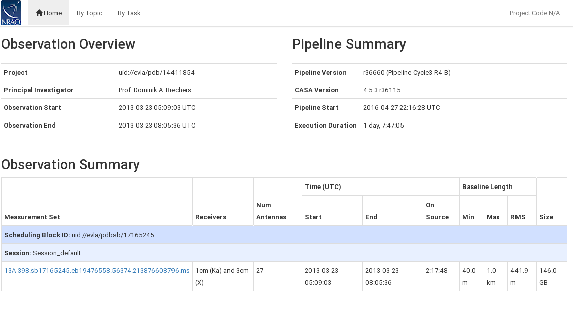
Overview Screen
An overview of the observations (Fig. 2) can be obtained by clicking on the MS name.
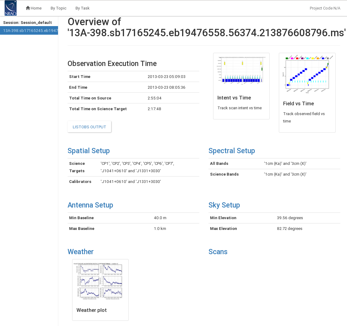
This page provides additional information about the observation. It includes Spatial Setup (field names, target and calibrator names), Antenna Setup (min/max baseline lengths), Spectral Setup (band designations; science bands include most calibrators but exclude ancillary scans such as pointing scans), and Sky Setup (min/max elevation). The page also provides graphical overviews of the scan intent and field ID observing sequence. A plot with weather information is also provided. Clicking the blue headers provides additional information on each topic.
The Spatial Setup page (Fig. 3) lists all sources and fields (where a source is a field with a given spectral setup). Names, IDs, positions, and scan intents are listed for each source/field.
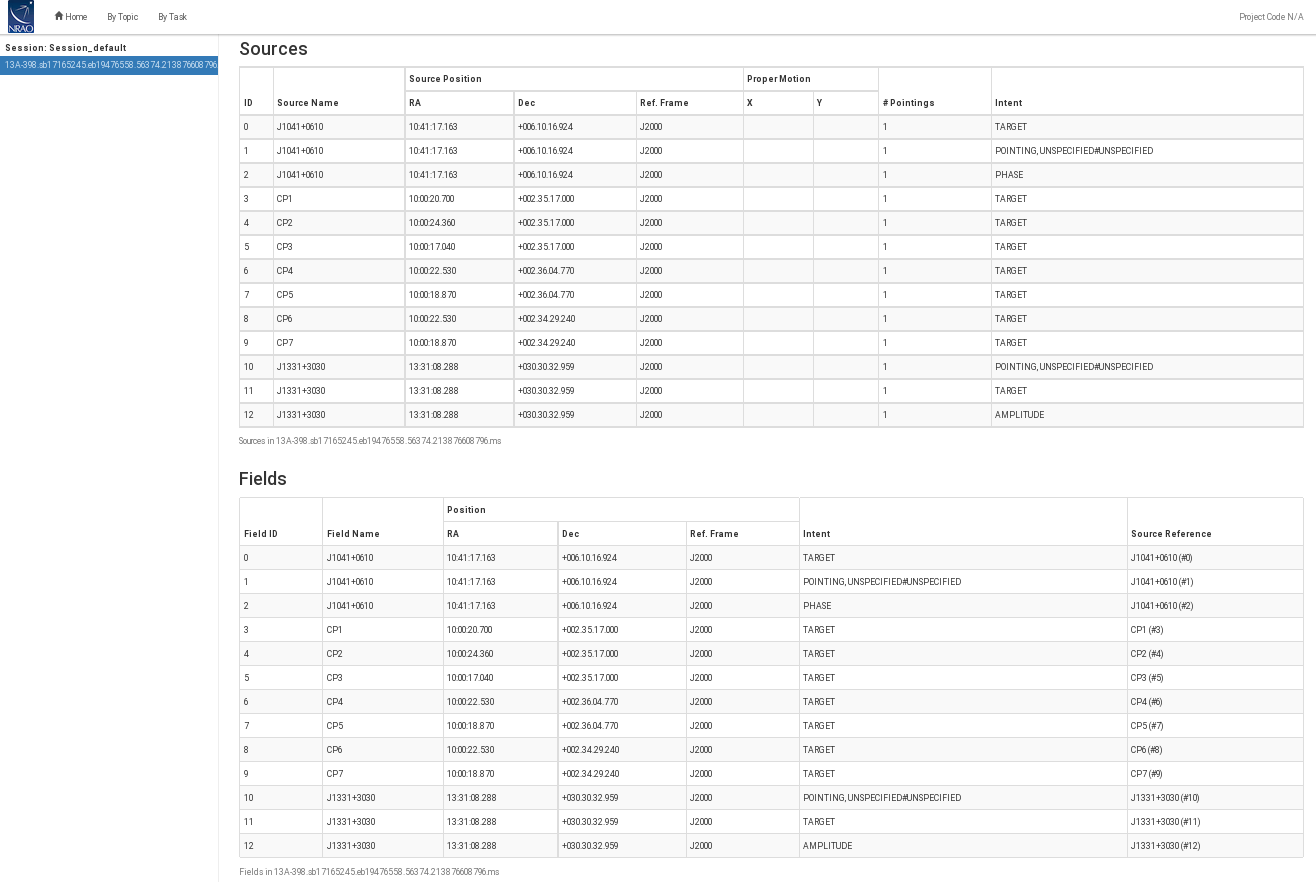 |
The Antenna Setup (Fig. 4) page lists the locations of all antennas (antenna pad name and offset from array center) and contains a graphical location plot for the array configuration. On a second tab, baseline lengths are listed and the 'percentile' column provides a rough indication of how many baselines are shorter than that in each row.
 |
 |
The Spectral Setup page (Fig. 5) contains all spectral window descriptions, including start, center and end frequencies, the bandwidth of each spectral window (spw), as well as the number of spectral channels and their widths in frequency and velocity units. For each spw the polarization products and the receiver bands are listed, too.
Note that Science Windows contain all spws that are used for calibration. Setup and pointing scans are not part of science windows but they are available under All Windows together with their intents. (Note though that in our case, however, pointing scans are mistakenly identified as science scans, this is due to its peculiar data structure).
 |
Clicking the Sky Setup page (Fig. 6) leads to elevation versus Azimuth and Elevation versus Time plots for the entire observation. The plots are colorized by field and intent.
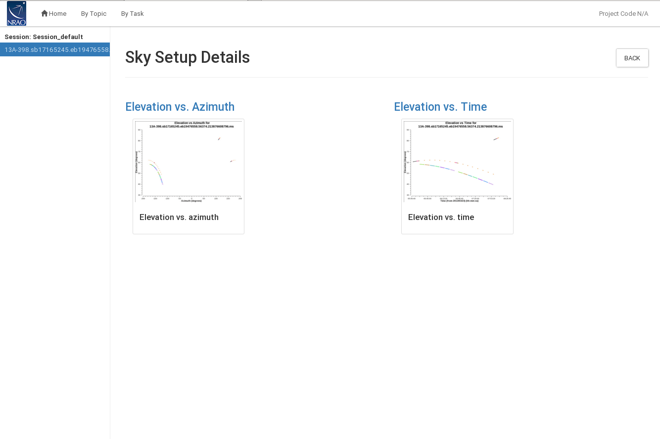 |
Scans (Fig. 7) provides a listing of all scans, including start and stop time stamps, durations, field names and intents, and the tuning (spw) setup for each. Again Science Scans and All Scans can be inspected in separate tabs.
 |
Most of the above information can also be accessed by the 'LISTOBS OUTPUT' button. The link leads to the output of thelistobs task, which lists the details of the observations (Fig. 8), including the scan characteristics, with observing times, scan ids, field ids and names, associated spectral windows, integration times, and scan intents. Further down, the spectral window characteristics are provided through their ids, channel numbers, channel widths, start and central frequencies. Sources and antenna locations are part of the listobs output, too.
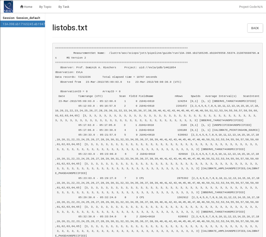
By Topic Screen
The top-level By Topic link leads to a page that provides basic pipeline summaries such as warnings, scores and flagging summaries as functions of field, antenna, and spectral window (spw) (Fig. 9).
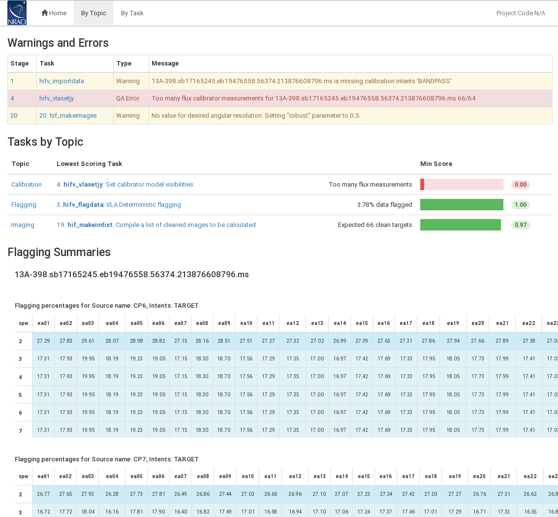
By Task Screen: Overview of the Pipeline Heuristic Stages
The pipeline is divided into 20 individual pipeline heuristic stages with heuristic ('hifv') tasks listed under the By Task tab (Fig. 10). Each stage has an associated score for success, but note that the scores are not yet implemented as of the CASA 4.5.3 VLA pipeline. Warnings and errors in tasks are indicated by 'exclamation mark' and 'cross' icons near the task names. In our example, the pipeline threw warnings during stages 1 and 20, and an error in stage 4.

To obtain more details on each stage, click on the individual task names. Task sub-pages contain task results such as plots or derived numbers. Common to all pages is information on the (Pipeline QA; 'Quality Assurance', not implemented in the CASA VLA pipeline as packaged in 4.5.3), the heuristic task Input Parameters, Task Execution Statistics (benchmarks), and the CASA logs. Those sections provide information on the triggered heursitics, as well as the actual CASA task execution commands and their return logger messages.
The Individual Stages
Stage 1. hifv_importdata: Register VLA measurement sets with the pipeline
In the first stage, the raw SDM-BDF is imported to a CASA MS. Basic information on the MS is provided, such as SchedBlock ID, the number of scans and fields and the size of the MS. The MS is also checked for suitable scan intents and a summary of the initial flags is calculated. In our example (Fig. 11), a warning is issued that the data does not contain a CALIBRATE_BANDPASS scan intent. In such a situation, the pipeline will use the flux density calibrator scans (marked by the CALIBRATE_FLUX intent) for bandpass calibration.
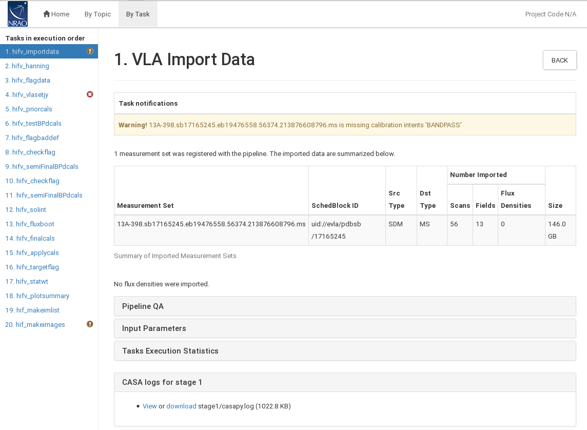 |
CHECK for: any errors in the import stage. That includes missing scan intents similar to our example. Warnings will also be issued if the data were previously being processed, this is usually encountered when the pipeline is run on an MS rather than an SDM.
Stage 2. hifv_hanning: VLA Hanning Smoothing
This stage Hanning-smoothes the MS. This procedure will reduce the Gibbs phenomenon (ringing) when extremely bright and narrow spectral features are present and spill over into adjacent spectral channels. Gibbs ringing is typically caused by strong RFI or a strong maser line. As part of the process, Hanning smoothing will reduce the spectral resolution.
CHECK for: nothing except for completion of the task. FOR SPECTRAL LINE DATA: you may decide not to run this stage since spectral lines will be smoothed to a degraded spectral resolution (see section on spectral line processing below).
Stage 3. hifv_flagdata: VLA Deterministic flagging
This stage will apply flags that were generated by the VLA online system during the observations. They include antennas not on source (ANOS), shadowed antennas, scans with intents that are of no use for the pipeline such as pointing and setup scans, autocorrelations, the first and last 5% edge channels of each spectral window (spw; with a minimum of 3), clipping absolute zero values that the correlator occasionally produces, quacking (ie flagging start or end integrations of scans; the pipeline will flag the first integration after a field change), and flagging the end 10 channels of the top and bottom spw of each baseband. The flags are reported as a fraction of the total data for the full dataset as well as broken up into the individual calibrator scans and target data. A plot is provided that displays the online antenna flags as a function of time.
In our example (Fig. 12), the target sources start with 3.12% flagged data; the deterministic flagging stage adds 6.05% for antenna not on source; 0.82% of other online flags (e.g., subreflector rotations or translations); edge channels amount to 6.4%; clipping of absolute zero values to 0.09%; and 1.40% of flags are due to baseband clipping. This combines to a total of 8.71% of flagged data for the scientific targets. Other sources are also listed and the entire MS is flagged on a 8.84% level.
 |
CHECK for: the percentage of the flags. If a very large portion (or even all) of the visibilities of the calibrators are flagged, try to find out the reason. Also have a quick look at the graph of the online flags to understand whether the system behaved normally or if there was an unusually high failure of some kind.
Stage 4. hifv_setjy: Set calibrator model visibilities
Stage number 4 calculates and sets the calibrator spectral and spatial model for the standard VLA flux density calibrators (3C48, 3C138, 3C147, or 3C286 with a CALIBRATE_FLUX scan intent). The task page lists the calculated flux densities for each spectral window (spw). It also contains plots of the amplitude versus uv-distance for the models per spw that are calculated and used to specify the flux density calibrator characteristics. If the scan intent CALIBRATE_FLUX is absent or the calibrator not a standard VLA flux density calibrator, the absolute calibration will be on an arbitrary level.
In our case, hifv_setjy throws an error (QA Too many flux calibrator measurements for 13A-398.sb17165245.eb19476558.56374.213876608796.ms 66/64; Fig. 13), which is due to the inclusion of pointing scans that are later disregarded. This is nothing to worry about here as the X-band pointing scans are not used for any scientific application. Pointing corrections are calculated and applied in the online system at the time of observation and are not used thereafter.
 |
CHECK for: any unexpected flux densities or model shapes.
Stage 5. hifv_priorcals: Priorcals (gaincurves, opacities, antenna positions corrections and rq gains)
Next, the prior calibration tables are being derived. They include gain-elevation dependencies, atmospheric opacity corrections, antenna offset corrections, and requantizer (rq) gains. They are independent of the calibrator observations themselves and can be derived from ancillary data such as antenna offset tables, weather data, antenna elevation, and switched power measurements.
In addition to the opacities themselves (calculated per spw; Fig. 14), a plot is attached that provides more information on the weather conditions during the observation.
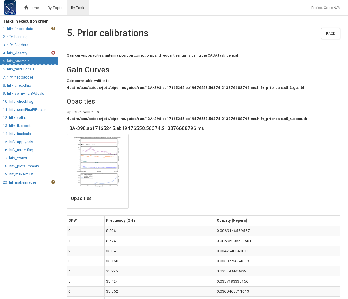 |
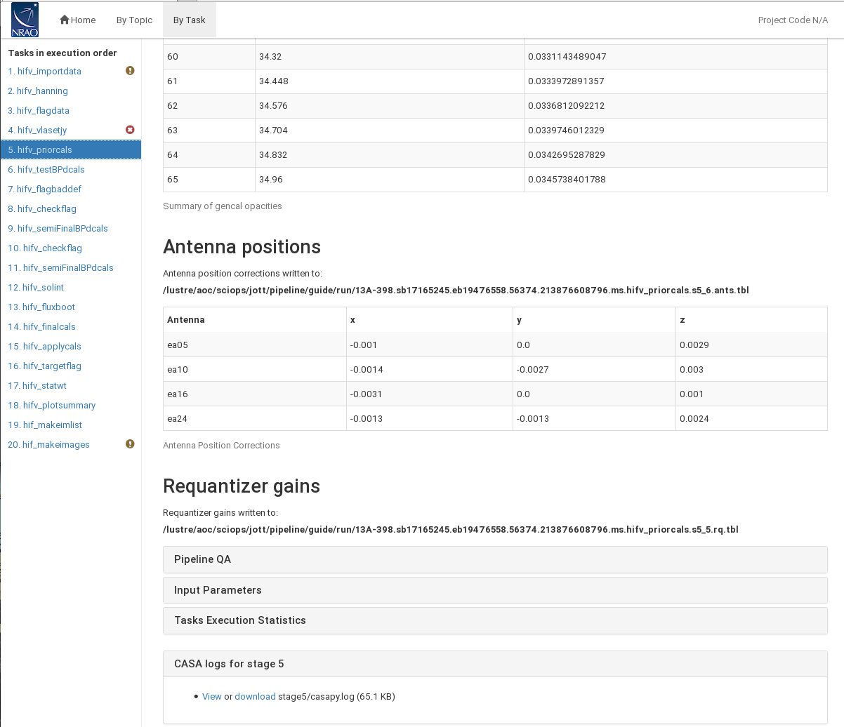 |
The antenna positions are usually updated within a few days after an antenna was moved, and for our case corrections (on the order of a few millimeters) for four antennas are applied.
CHECK for: extreme or unrealistic opacities. Also check that the antenna offsets are within are reasonable (reasonable values are usually less than +/- 0.0200 meters). There should only be updates for a few antennas.
Stage 6. hifv_testBPdcals: Initial test calibrations
Now it is time to determine the delays, and the bandpass solution (gain and phase) for the first time. Applying the initial solution will make it easier to identify RFI that needs to be flagged. There will be a couple of similar iterations for the calibration tables in the following pipeline stages to eventually obtain the final set of calibration tables.
The plot on the main page (Fig. 15) shows the bandpass calibrator with the initial bandpass solution applied. There are links to other plots showing delay, gain amplitude, gain phase, bandpass amplitude, and bandpass phase solutions for each antenna. Note that, when using a single reference antenna and a point source,
the phases must be zero (we will later see an example where a few antennas are used for reference). This will show up as steps in the phase plots. When delays are more than +/-10ns it will be worth examining the data more closely. Some additional flagging may be needed.
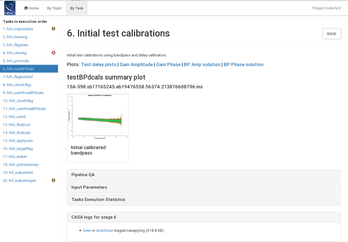 |
The gain amplitude and phase solutions are derived per integration and they are used to correct for decorrelation before any spectral bandpass solutions are calculated. The latter are determined over a full solution interval, usually for all bandpass scans together. Bandpasses should be smooth although they can vary substantially over wide frequency bands. The bandpass (BP) phase solutions calibrate the residual phases after the delays were calibrated.
Example delays are shown in Fig. 16: The delay for ea16 varies but is within a narrow range of only a few ns. These are good solutions. The delays for ea21 are fine except for the 33-35GHz frequency range where they scatter substantially. The respective frequency range/spectral window (spw) should be flagged manually if the following pipeline steps will not take care of it. For ea22 the delays in the 35-37GHz range are excessive with a value of about -70ns. It is likely that the pipeline will be able to calibrate these values correctly but one may need to flag the respective spws if not.
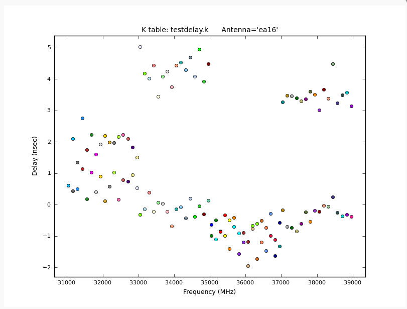 |
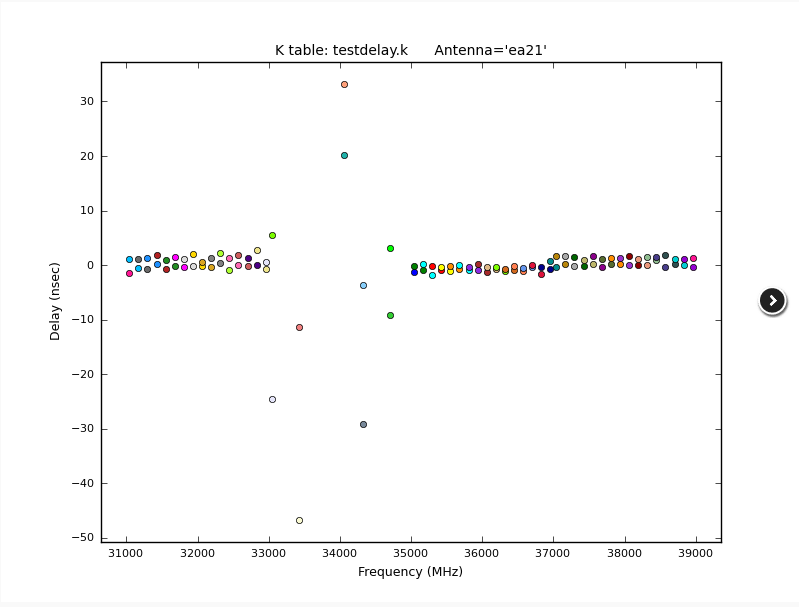 |
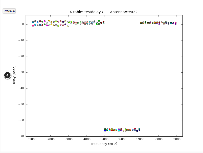 |
In Fig. 17, we show some of gain amplitude plot examples. Antenna ea03 shows credible solutions (the colors represent different spectral windows and polarizations and a flux spread as a function of frequency is expected), whereas ea04 has elevated values until 8:06. Those should be flagged (but the pipeline may be able to detect and flag them in one of the subsequent stages). Some of the baselines in ea18 show low values in the 2-3Jy range, but they are constant in time. At this stage one can assume that they reflect the correct calibration values. It might still be worth making a note and check if calibration downstream was applied correctly. The situation is different for ea25 which shows an extreme decrease of amplitude as a function of time. This is likely an antenna mechanical error. This antenna should be inspected carefully, there could be a problem which will make it unusable. Although the bandpass solutions seem to be ok, the bandpass and flux calibrators coincide and it is likely that the absolute flux density calibration is very unreliable for this antenna.
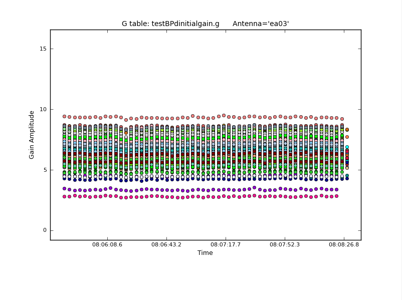 |
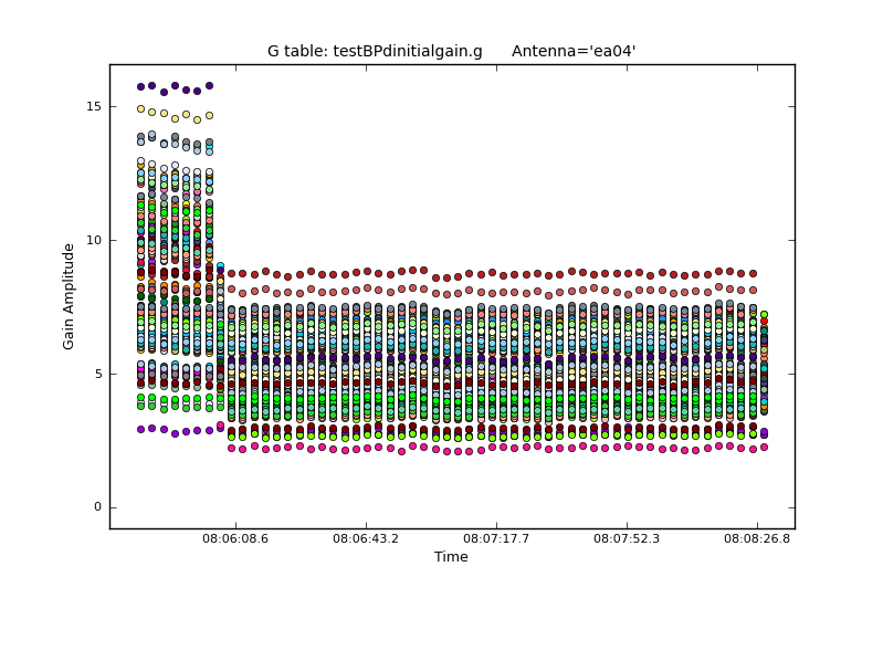 |
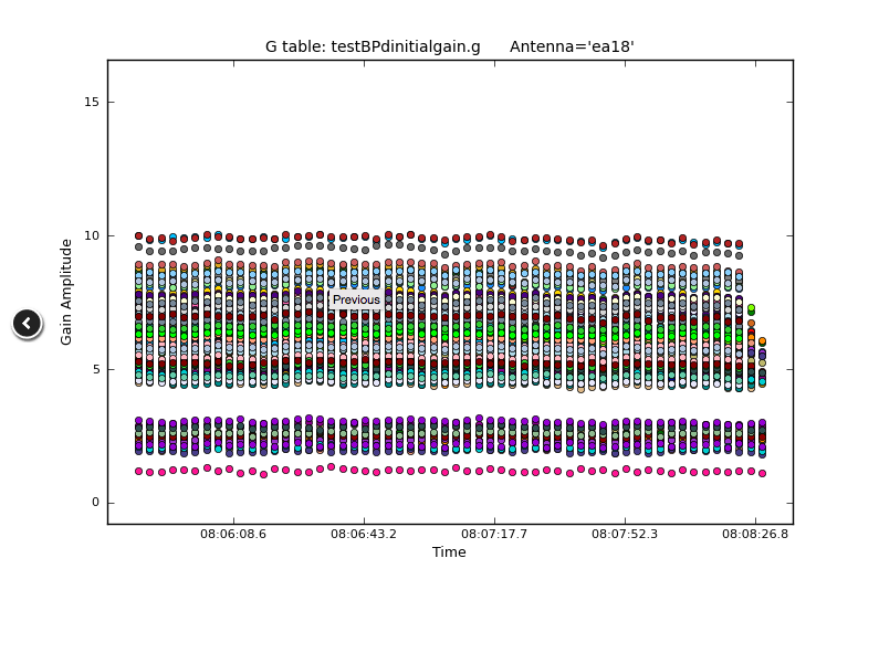 |
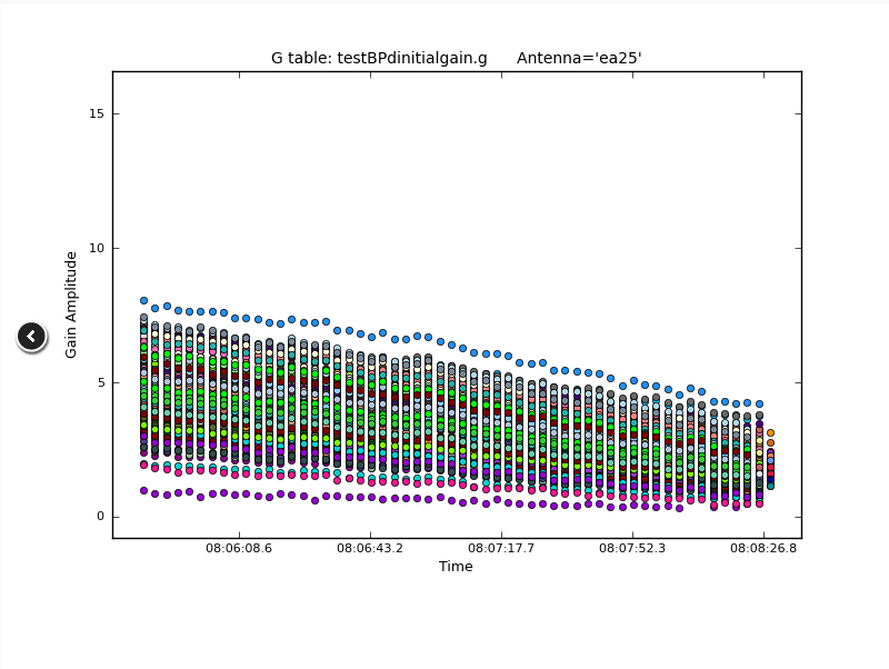 |
Since the gain amp/phase steps per integration are only performed to reduce decorrelation, the phase plots are the most important in this context. In Fig. 18 we show a few solutions. All phases for the reference antenna ea09 are by definition zero. The phase variations as a function of time increase for higher frequencies and longer baselines. Therefore both, ea03 and ea21 have good solutions given that ea03 is closer to ea09 than ea21 (cf. the Antenna Setup on the Overview page). There are no jumps in the phases - remember that -180 and +180 are identical phase values and lines connecting those values are only a plotting issue, not the actual phase behavior.
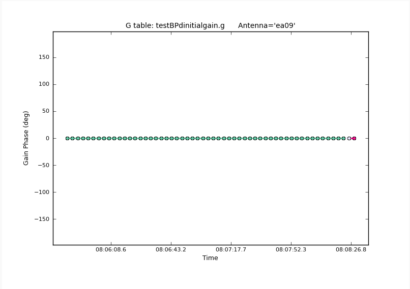 |
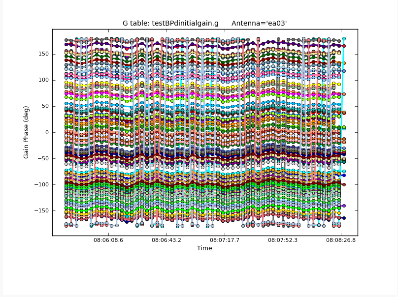 |
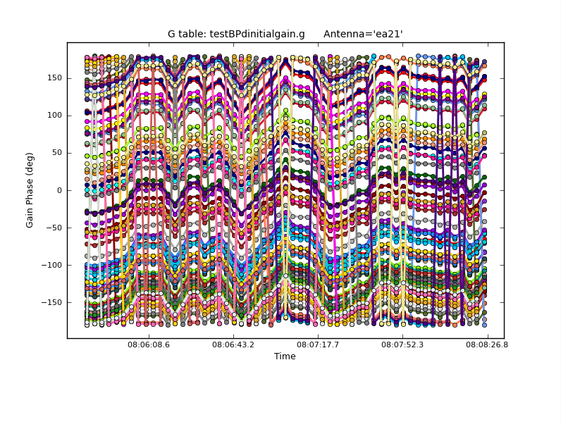 |
Now let's have a look at the bandpasses themselves (Fig. 19). Antenna ea17 shows very good bandpass solutions. Since the spectral windows (spws) are small compared to the entire frequency range, the edges of each spw dominate the variations. The 37-39GHz range of ea18 varies considerably more. In fact this antenna, polarization and baseband shows a deformatter timing error (more in the following stage 7) which needs to be flagged. Some flagging was already performed for the 33-35GHz range of ea21. This range corresponds to the noisy delays that we saw earlier in Fig. 16b. Antenna ea24 shows a few high values. They usually are fine as they also correspond to the edges of the spws. In particular if an spw edge coincides with a baseband edge, such spikes are usually more pronounced. Keep an eye on those although they are likely not a problem for the calibration. Finally, we show the bandpass of ea25, the antenna with the likely mechanical error. Although the Gain Amplitude showed decreasing values as a function of time (Fig. 17d), the bandpass itself does not look suspicious and can likely be used, based on this plot. The mechanical error, however, may also be present for other scans and since we identified it first for a flux density calibrator scan, that antenna should be flagged.
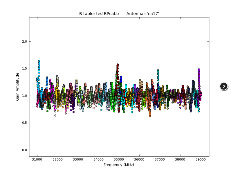 |
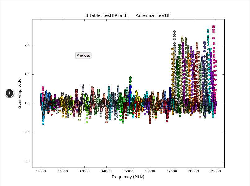 |
 |
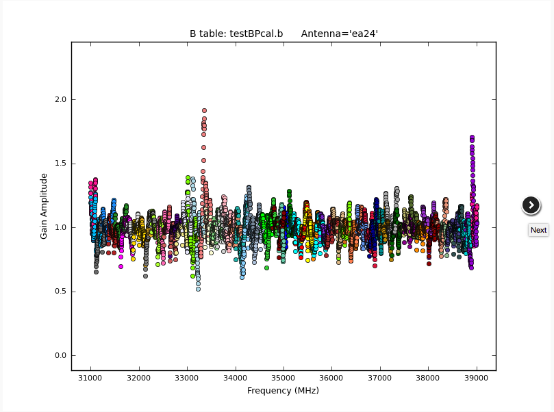 |
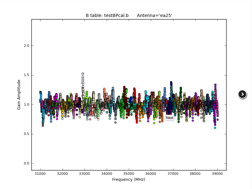 |
The bandpass (BP) phases (Fig. 20) show residual, channel by channel phases. Again the reference antenna ea09 only shows zero phases by definition. Antenna ea11 is an example of proper phase solutions across the bandpass. Note again that the variations are dominated by residual phases at the edges of the spectral windows. Some variations are larger than others, but they are all in a similar range. We already saw the large scatter in the bandpass amplitude of ea18 at 37-39GHz due to a signal path (bad deformatter) problem and the pattern is apparent in the phases. Finally we show ea24 again and find that the edge spike in the amplitudes is also seen in the phases. At this level, the solution should be usable.
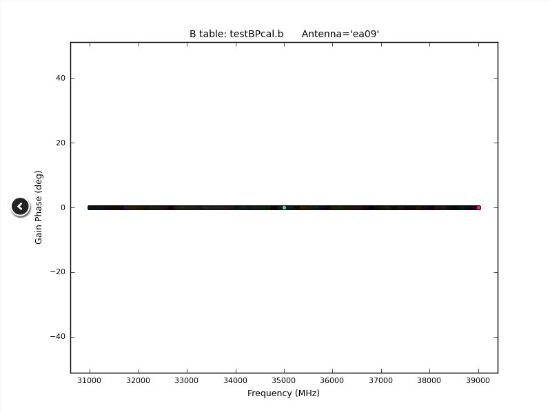 |
 |
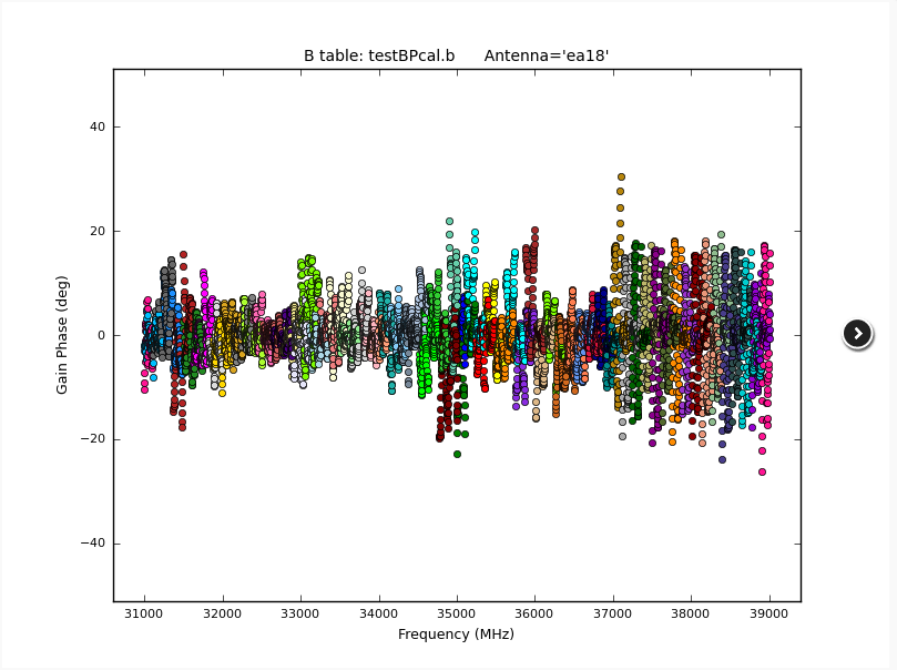 |
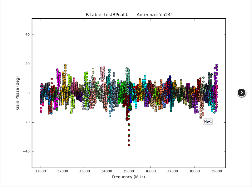 |
CHECK for: strong RFI and whether it was eliminated in later flagging stages or not (especially via a comparison with the output plots of task 14). Also check for jumps in phase and/or amplitude away from spectral window edges. If there are phase jumps for all but the reference antenna, maybe a different choice for the reference antenna should be considered. Also watch out for extreme delays of tens of ns and for very noisy data.
Stage 7. hifv_flagbaddef: Flag bad deformatters
The digital transmission system (DTS) of each VLA antenna includes a formatting stage to convert the electronic to an optical signal before it is injected on the optical fiber link. On the correlator end the signal will be deformatted back to an electronic signal. Occasionally, the timing on the deformatter can be misaligned which results in very strong amplitude or phase slopes as a function of frequency. Sometimes the signal is similar to an abs(sin), or a 'bouncing' signal across a baseband for one polarization. The hifv_flagbaddef pipeline stage tries to identify such deformatter errors by checking for deviations more than 15% over the average bandpass. In that case the antenna, polarization, and spectral window (spw) are flagged. If more than 4 spws of a baseband are affected this way, the entire baseband will be flagged.
For our data, no deformatter issues were automatically detected in the data for the amplitudes but the phases of a few spws are flagged (Fig. 21). We did see, however, that ea18 has a DTS problem in the 37-39GHz baseband (Figs. 19b/22a and 20c). Since this stage 7 did not detect and flag this range (which shows the limitations of the underlying code), manual flagging will be required for the affected antenna, polarization, and baseband for all sources. An example from a different dataset is provided in Fig. 22b. The 'V' shape close to 5.3 GHz with some values reaching close to zero are a sign for a deformatter problem.
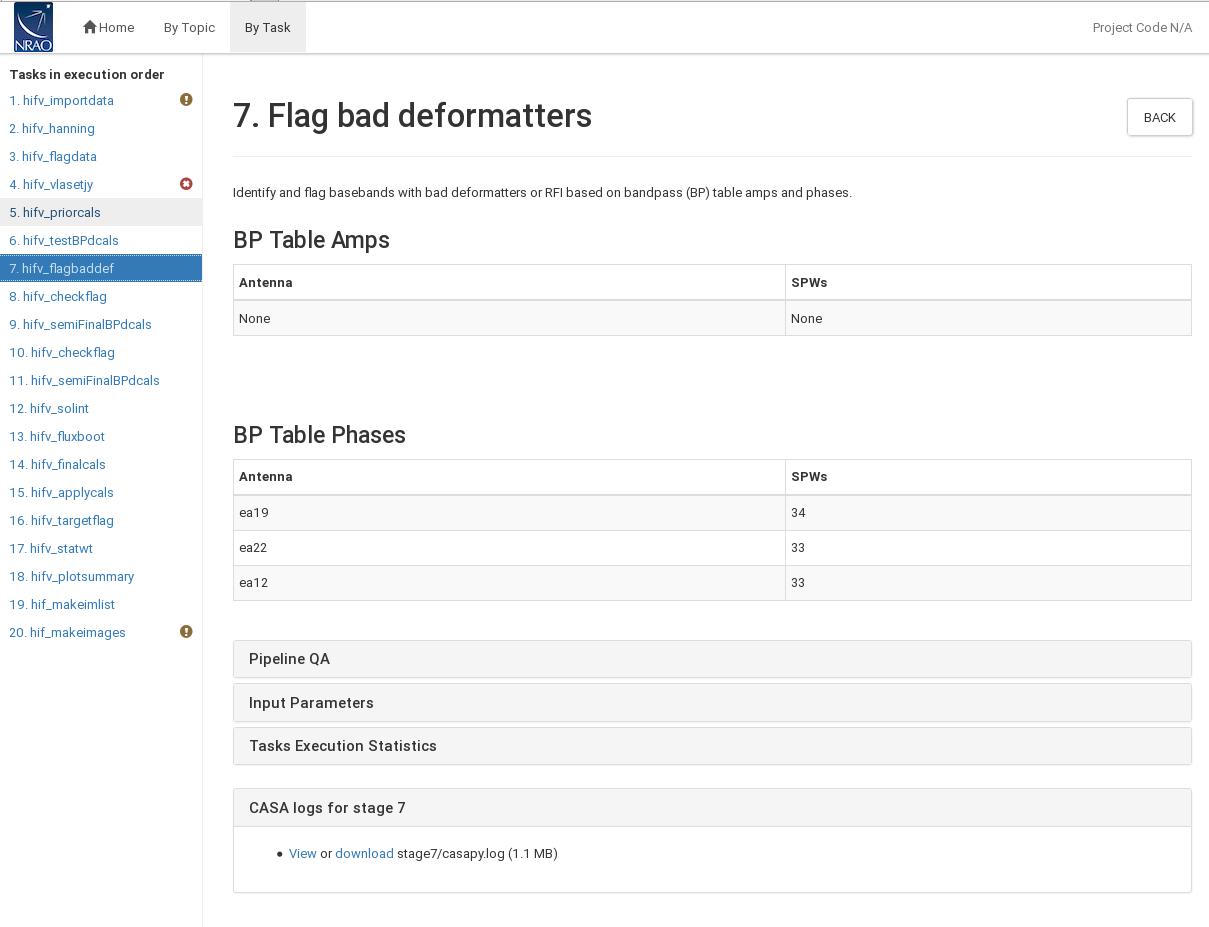 |
 |
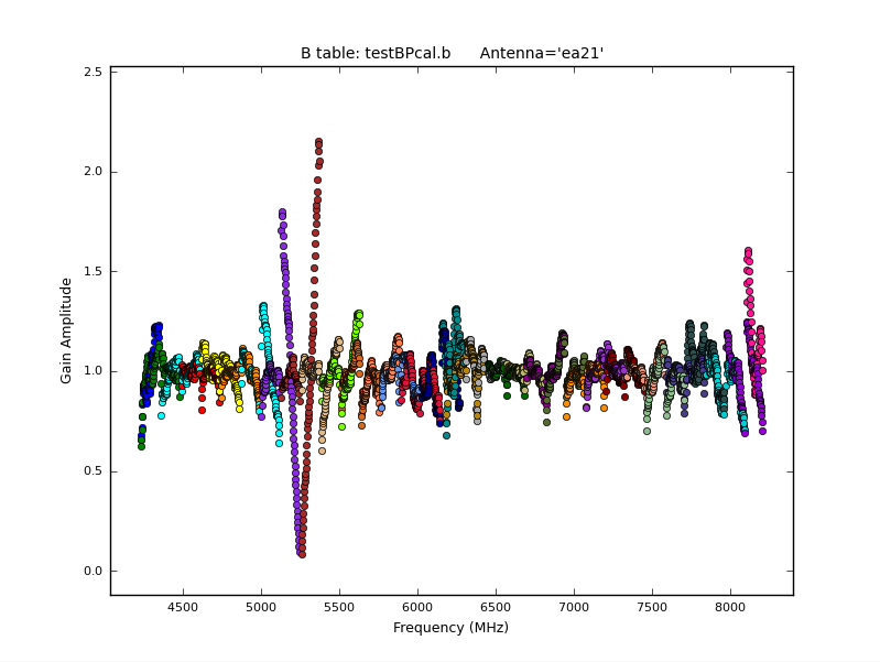 |
CHECK for: amplitude 'bounces', i.e. very strong variations of amplitude and/or phase well above the average of the other polarizations or basebands. The pattern can repeat a few times across a baseband but should be contained to a single baseband, antenna and polarization. Data for all sources in the spectral windows in a faulty baseband are
affected.
Stage 8. hifv_checkflag: Flag possible RFI on BP calibrator using rflag
Rflag as part of flagdata is a threshold-based automatic flagging algorithm in CASA. In this step, rflag is run on the bandpass calibrator to remove relatively bright RFI and to obtain improved bandpass calibrations tables later on.
CHECK for: nothing in particular on this page, but some cumbersome RFI may have been eliminated in preparation for the following steps.
Stage 9. hifv_semiFinalBPdcals: Semi-final delay and bandpass calibrations
Now that some RFI was flagged, stage 6 is repeated here at stage 9, which results in better bandpass and delay solutions.
CHECK for: strong RFI and whether it was eliminated in later flagging stages or not (especially via a comparison with the output plots of task 14). Also check for jumps in phase and/or amplitude away from spectral window edges. If there are phase jumps for all but the reference antenna, maybe a different choice for the reference antenna should be considered. Also watch out for extreme delays of tens of ns and for very noisy data.
Stage 10. hifv_checkflag: Flag possible RFI on BP calibrator using rflag
Once more, rflag is executed. After the bright RFI has been removed in step 8 and a new bandpass solution has been applied in step 9, a new flagging threshold will account for weaker RFI, which will be removed in this step 10.
CHECK for: check that RFI was removed in the following steps.
Stage 11. hifv_semiFinalBPdcals: Semi-final delay and bandpass calibrations
Again, having removed more RFI, new delay and bandpass solutions are obtained here.
CHECK for: strong RFI and whether it was eliminated in later flagging stages or not (especially via a comparison with the output plots of task 14). Also check for jumps in phase and/or amplitude away from spectral window edges. If there are phase jumps for all but the reference antenna, maybe a different choice for the reference antenna should be considered. Also watch out for extreme delays of tens of ns and for very noisy data.
Stage 12. hifv_solint: Determine solint and Test gain calibrations
For the final calibration, the pipeline determines the shortest and longest applicable solution interval (solint). Typically they refer to the (longest) visibility integration time and the length of the longest gain calibration scan, respectively.
In our case (Fig. 23) the longest time per integration is 3 seconds which therefore also corresponds the shortest solution interval. The longest solution interval is based on the longest phase calibrator scan, which lasts for ~85s. When subtracting the slew time and allowing for 'quack' flagging of the longest solution interval, the longest solution interval results in ~75s.
 |
Using these solution intervals, a temporal gain and phase solution is calculated for each antenna, spectral window, and polarization. In Fig. 24 we show some examples for the gains. Antenna ea03 shows consistent gain solutions with small variations over the time of the observations. Note that the last scan is the flux density calibrator and thus a different source with a different gain amplitude. Antenna ea04 shows increased values for the last few calibrator scans that may need to be flagged. Antenna ea25 has likely a pointing error that deteriorates over the first half of the observations. The listobs output tells us that a pointing update was obtained around 6:40 at which point ea25 indeed recovered and shows good solutions.
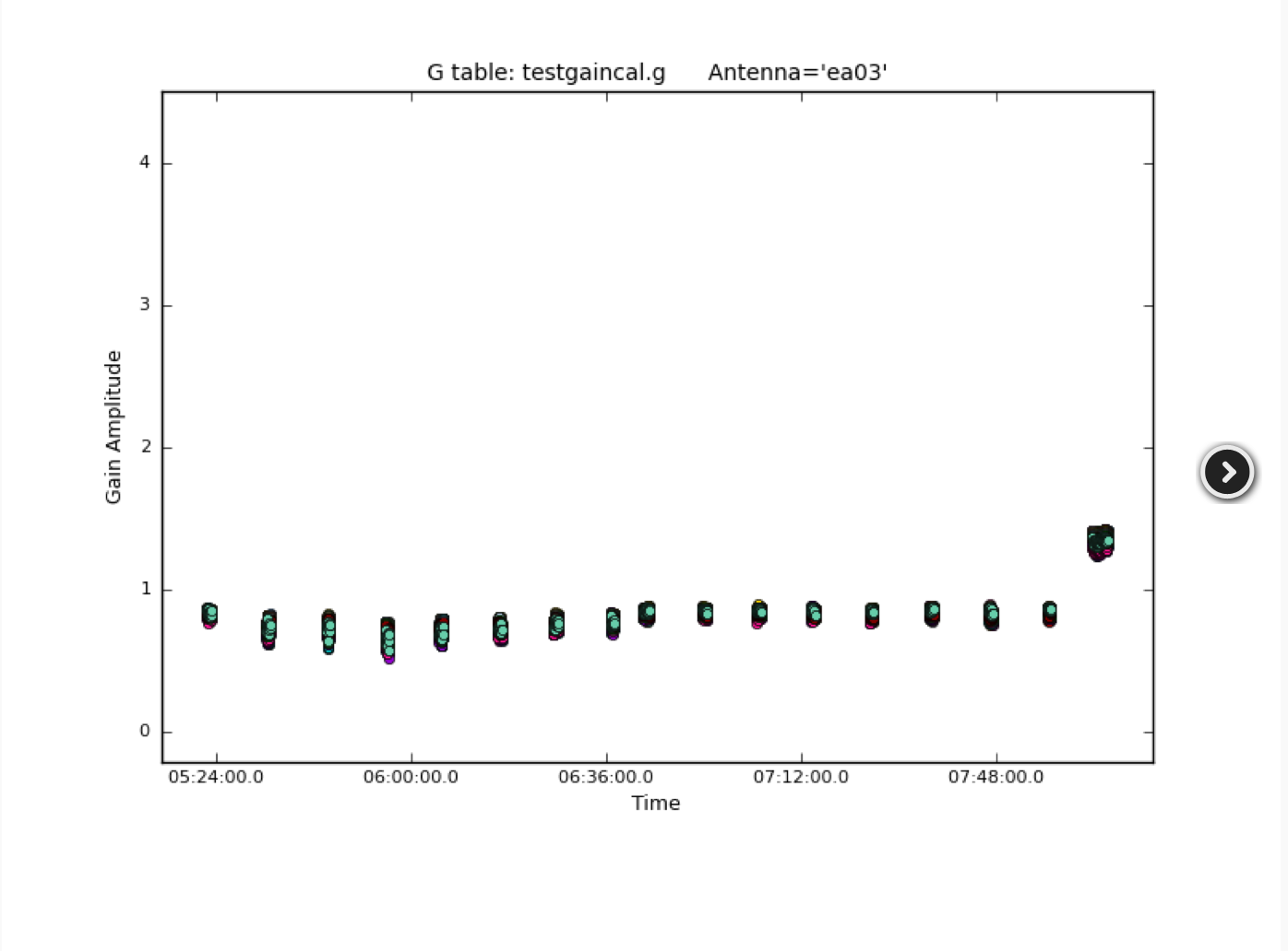 |
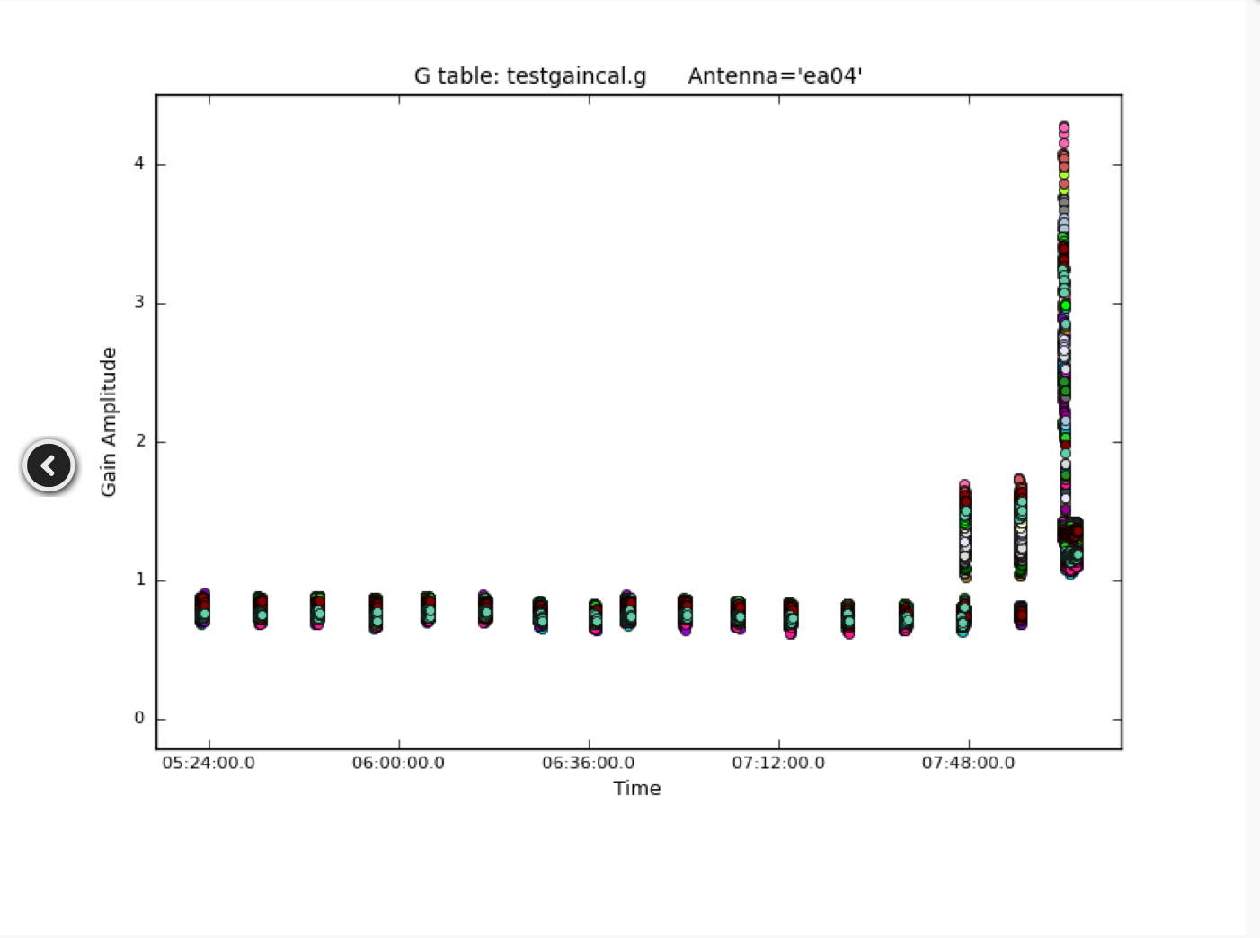 |
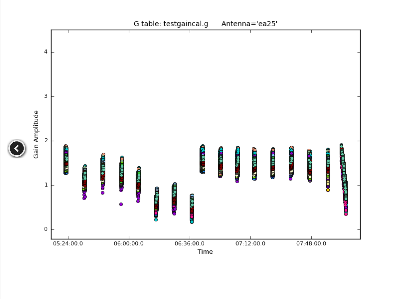 |
Although the phase solution plots are very crowded (Fig. 25), we can see that ea03 has very steady values over time. The pipeline will apply phase corrections that are determined from this solution, so later on, additional phase solutions will be close to zero. Antenna ea04 shows larger variations. Antenna ea09 is the initial phase reference antenna. The underlying gaincal command, however, was given a few possible reference antennas, ea09, ea14, ea13, ea03, in case a single reference is not usable for all times and spectral windows. Check the CASA log for stage 12 at the bottom for the actual command. Indeed gaincal decided to chose different reference antennas for the solutions as the CASA log reports. To keep the phase interpolation consistent, ea09 phases have to absorb the offsets introduced by the alternate reference antennas. This explains the plot that we see here, i.e., not a constant zero for
all spectral window phases.
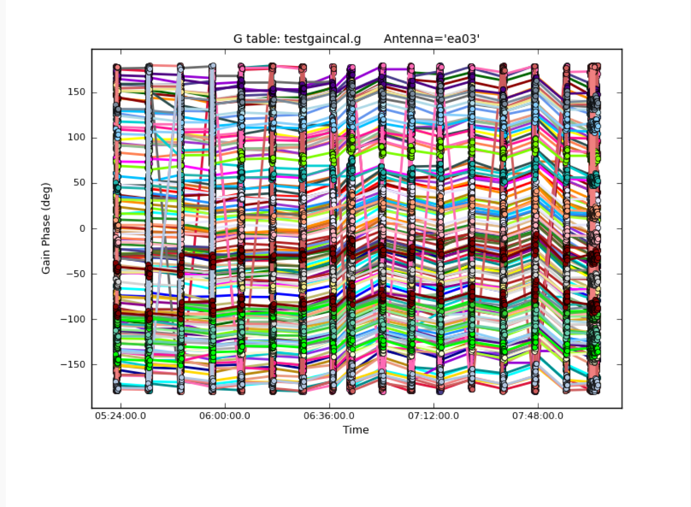 |
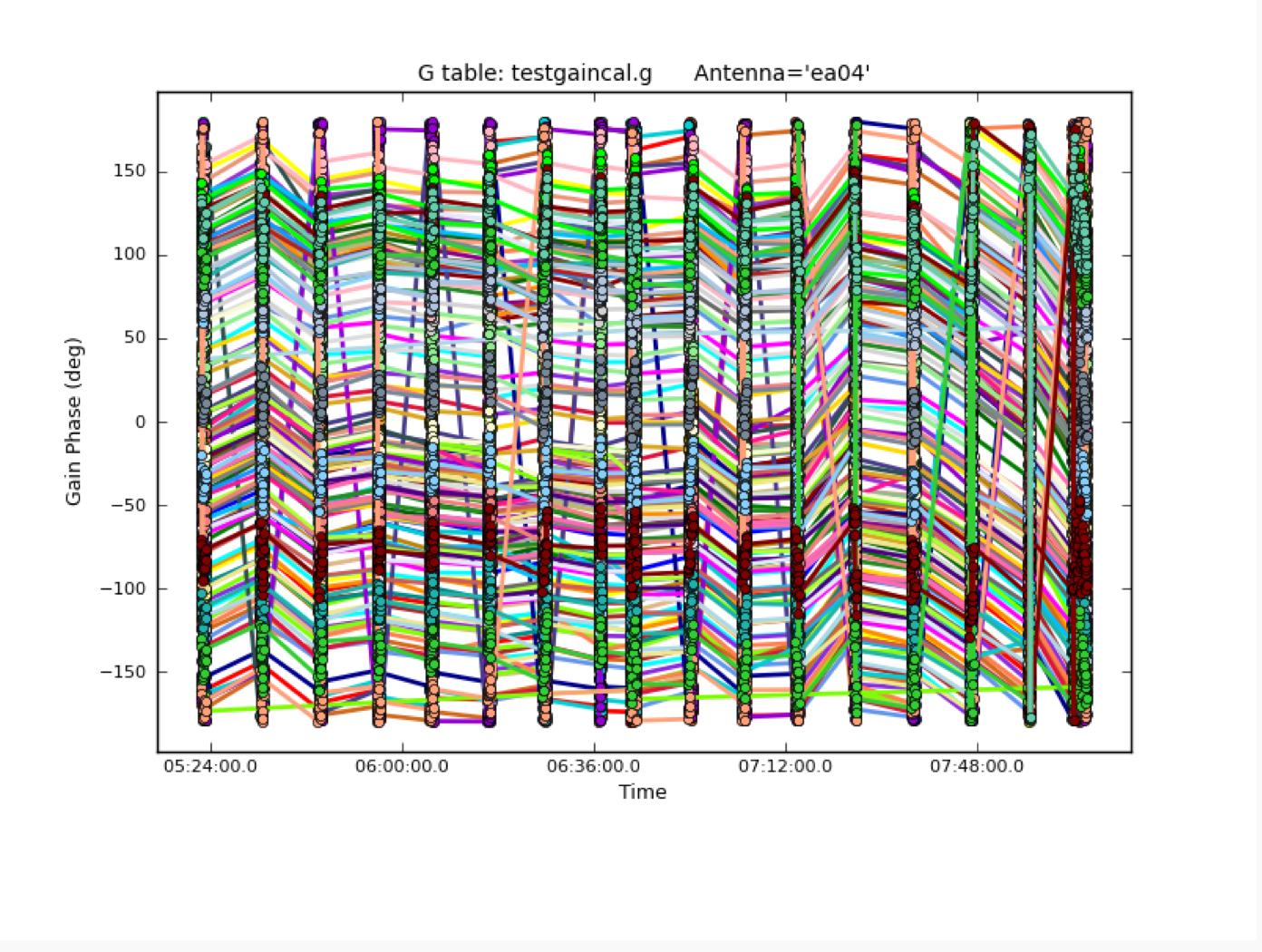 |
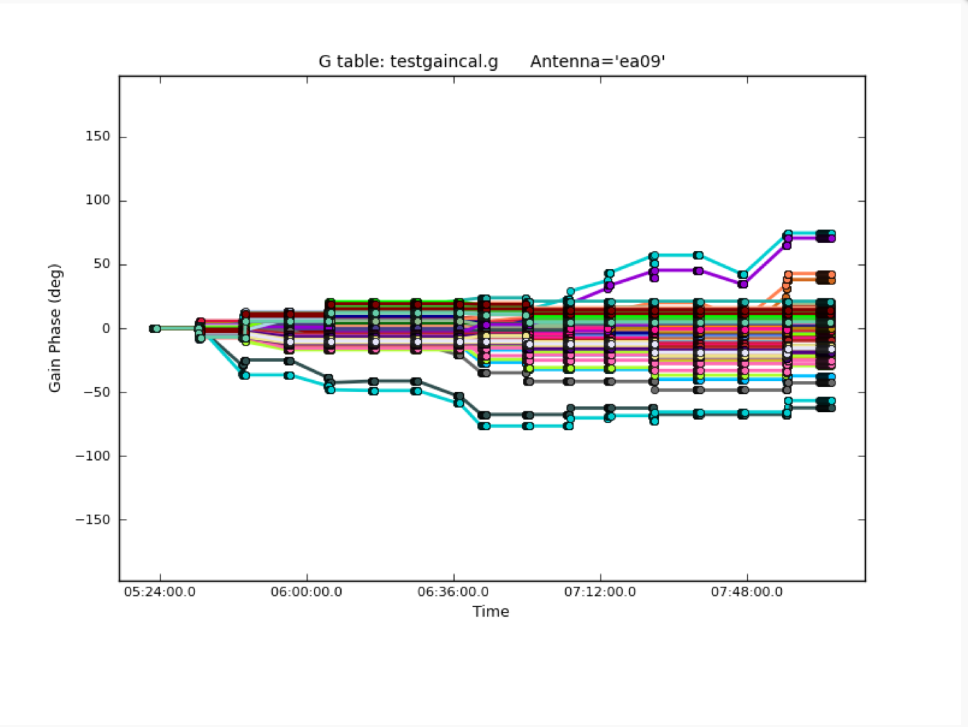 |
CHECK for: consistency with the data. The shortest solution interval should be close to the (longest) visibility integration time and the longest
gain calibration scan. Gains should be smooth with little variations in time (where larger gain variations are more likely to occur for higher
frequencies), phases should not show any jumps and should be relatively smooth in time (where larger phase variations are likely to occur for higher frequencies and longer baselines).
Stage 13. hifv_fluxboot: Gain table for flux density bootstrapping
Now, the fluxes are bootstrapped from the flux density calibrator to the complex gain (amplitude and phase) calibrator. To do so, spectral indices are computed for the secondary calibrator and the absolute flux densities are determined for each channel. They are then inserted in the MODEL column via setjy and reported for each spectral window.
For our example, the pipeline derives flux densities between 0.61 and 0.68 Jy for the phase calibrator, depending on frequency. The spectral behavior is reported as a declining spectral index of around -0.5 (Fig. 26). The plot also shows the models for both, the flux density and the bootstrapped gain calibrator.
 |
CHECK for: that the values are close to the known fluxes of the calibrator. Check the VLA calibrator manual at https://science.nrao.edu/facilities/vla/observing/callist for consistency. Since most calibrator sources are time variable AGN, some differences to the VLA catalog are expected. In particular at higher frequencies they could be up to tens of percent.
Stage 14. hifv_finalcals: Final Calibration Tables
The final calibration tables are now derived. Those are the most important ones as they are applied to the data in stage 15. The tables, which contain antenna based solutions, are: Final delay, bandpass (BP) initial gain phase, BP Amp solution, BP Phase solution, Phase (short) gain solution, Final amp time cal, Final amp freq cal, and Final phase gain cal. We have already inspected and discussed similar solutions for the bandpass and for the temporal gain/phase calibration earlier. We shall now investigate further, starting with the temporal gains.
The gains vary significantly for this observation. Typically, the gains stay within 10% around a normalized value of 1. Here, a few spectral windows (spws) show substantial deviations. Examples are (Fig. 27): Antenna ea02 has a drop around 5:50 and should be checked (also ea01 which is not shown). Maybe the entire time between the adjacent, good calibrator scans should be flagged for this antenna. Antenna ea04 has an inverse behavior later, around 8:00. It appears that only a subset, e.g., a baseband, deviates from the rest. Antenna ea07 is more smooth, with some variations between the individual spws but overall a consistent temporal behavior. Likely this solution can be used with no further flagging. Note that the last scan is the flux density calibrator. This scan is expected to have different gains than those for the complex gain calibrator. Next, note that the ea09 gains are almost unity, which is expected. The gains in ea18 are smooth with a large dip in the first half. This in fact does calibrate out some characteristics of the observations and could be left for the moment. As mentioned before, around 6:40, a pointing update was performed which seems to have rectified a possibly mis-pointed ea18. Antenna ea23 requires a single spectral window at a single time to be investigated and probably be flagged. The mechanical error that we have identified for the bandpass/flux calibrator scan using ea25 has affected the phase solutions. That explains the amplitude spread of the spws. In addition, this antenna also has a pointing error for the first half of the observation. We again recommend to flag the entire antenna.
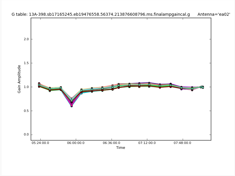 |
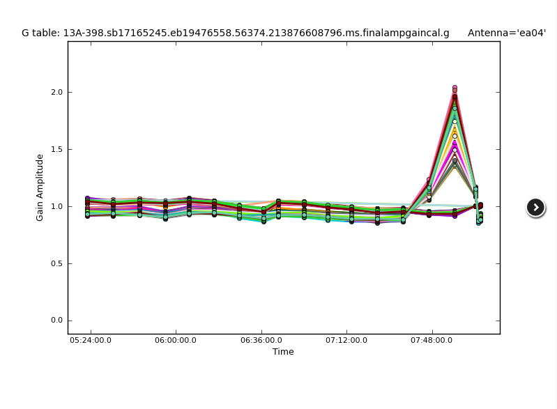 |
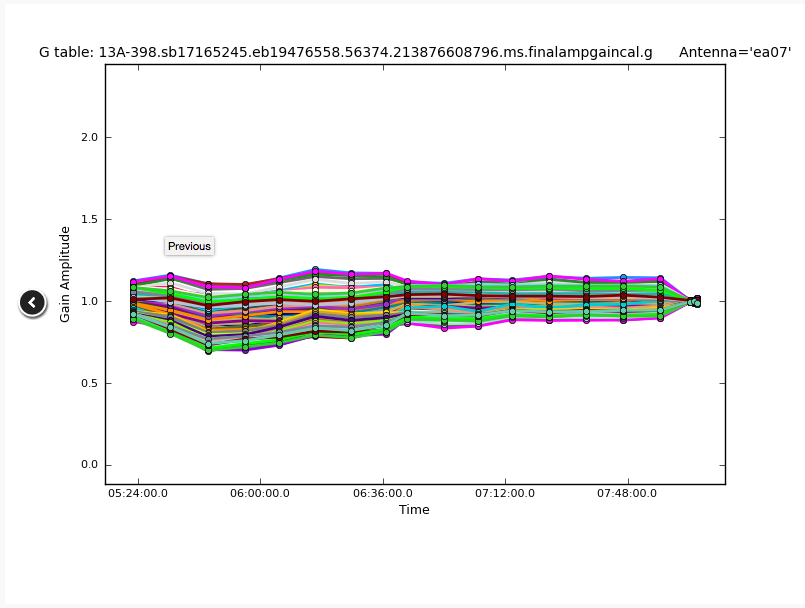 |
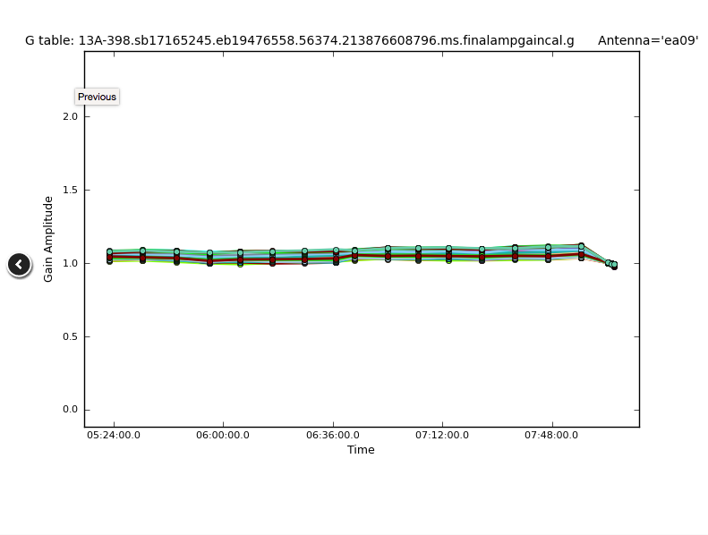 |
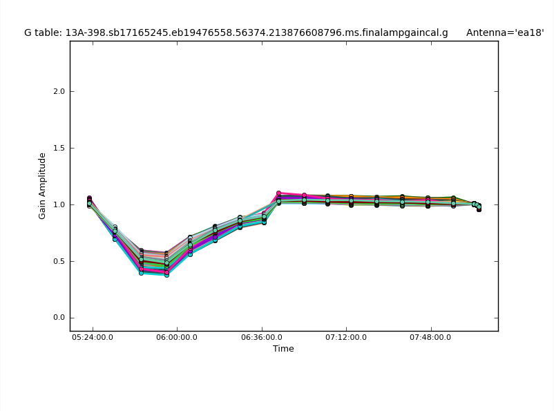 |
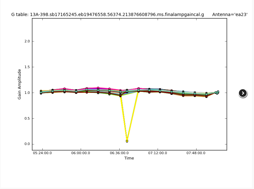 |
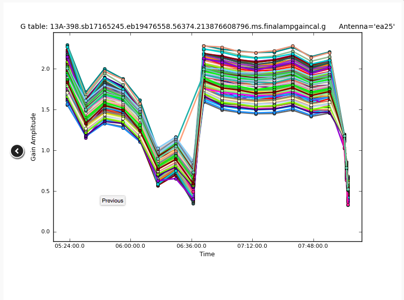 |
Now let's have a look at the gains as a function of frequency (Fig. 28). For ea02 we see that one line is below the rest. This is likely one specific time interval and indeed we have seen such a slip in Fig. 27a. Antenna ea04 has a very noisy time interval, which is also in agreement with what we have seen in the previous temporal gain plot. Antenna ea08 shows a consistent calibration and ea20 repeats the extra noise in the 34-35GHz range that may need to be flagged. Antenna ea25 now reflects the bandpass pattern that we have seen earlier and that explains the spread in Fig. 27.
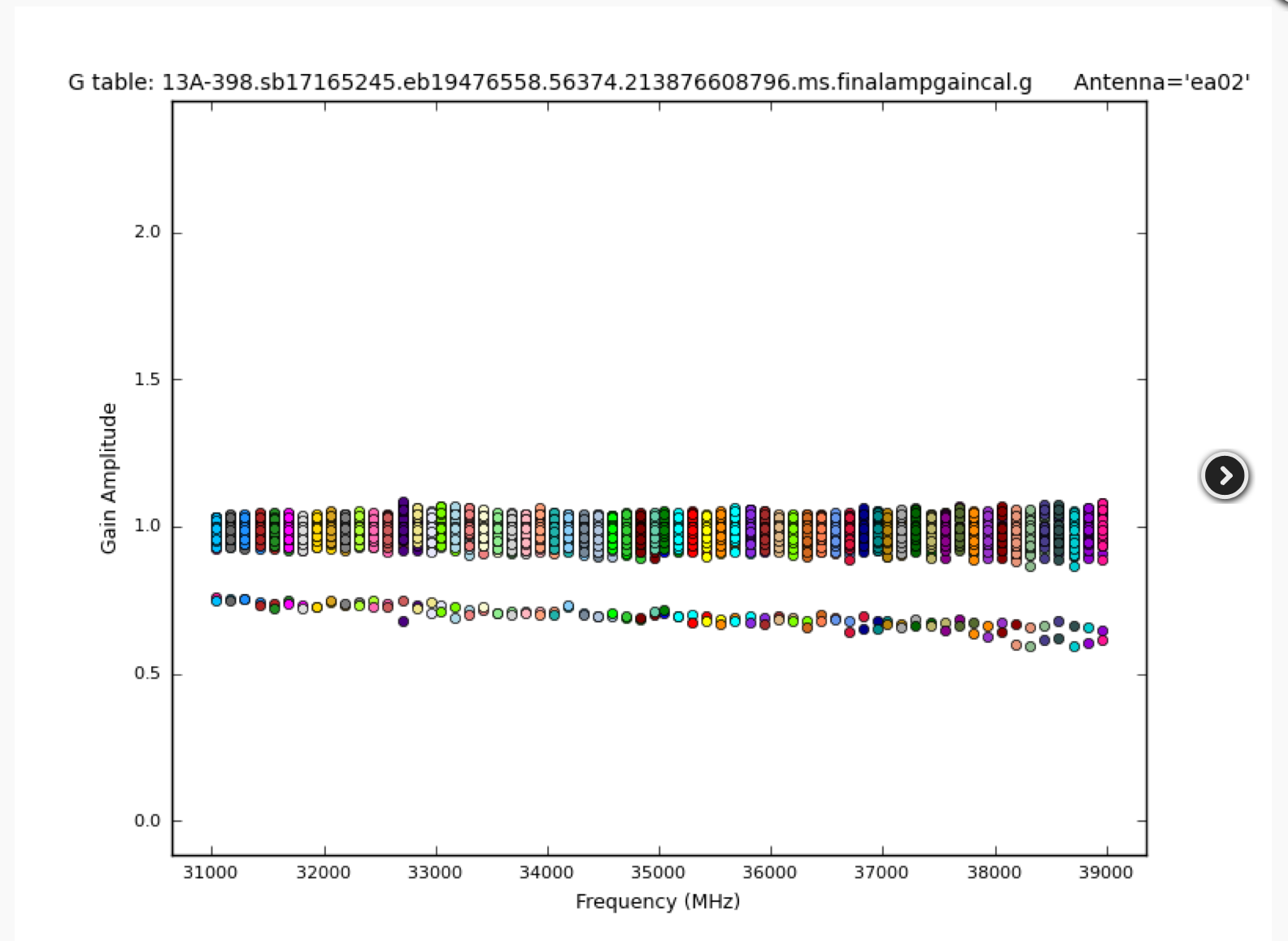 |
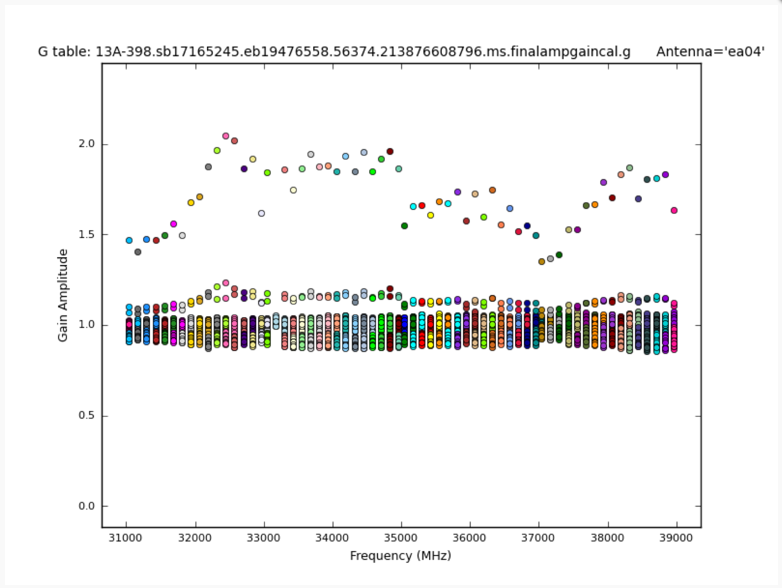 |
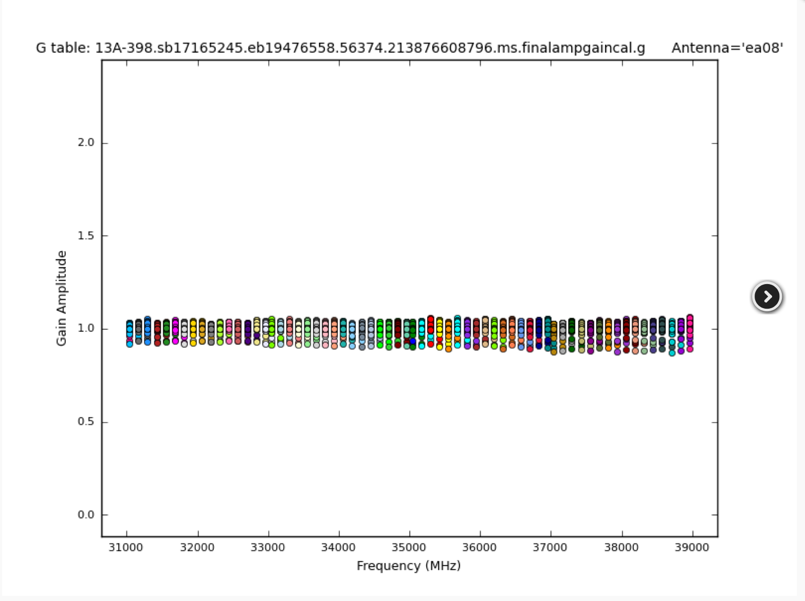 |
 |
 |
The phases versus time ("Final phase gain cal") are shown in Fig. 29. Antenna ea02 clearly shows very erratic phase variations for one baseband or polarization. This is likely not recoverable. The user may plot the solution in plotcal or plotms and locate the faulty spectral windows or polarizations and flag them. Antenna ea04, in contrast, exhibits very smooth phase variations until near the end of the observations. This has already been observed in the amplitude gains (Fig. 27b), should be looked at, and likely needs to be flagged. Antenna ea09 is the reference antenna and therefore has phase solutions that are zero as function of time. Antenna ea13 shows smooth variations and is an example for a credible calibration table. A spread between basebands or polarizations can be seen for ea15. The behavior is nevertheless smooth and the data should be calibrated nicely with this table. Antenna ea17, however, has, in addition to different behaviors for the basebands, also relatively large and erratic jumps between the calibration scans. This clearly needs to be looked into further and may require flagging, although the antenna did not show any issues in previous plots. Finally, ea20 has a relatively smooth behavior until the pointing update was performed (although the variations are relatively large). After the pointing scan, however, phases vary by about +/-50degree between individual, consecutive calibrator scans, which is large enough to be unreliable and to be flagged.
 |
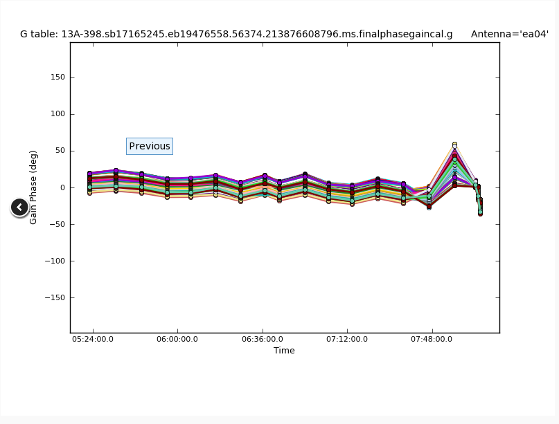 |
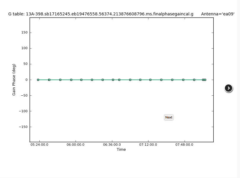 |
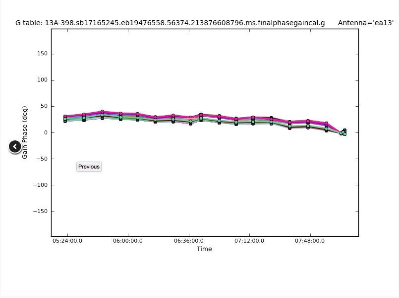 |
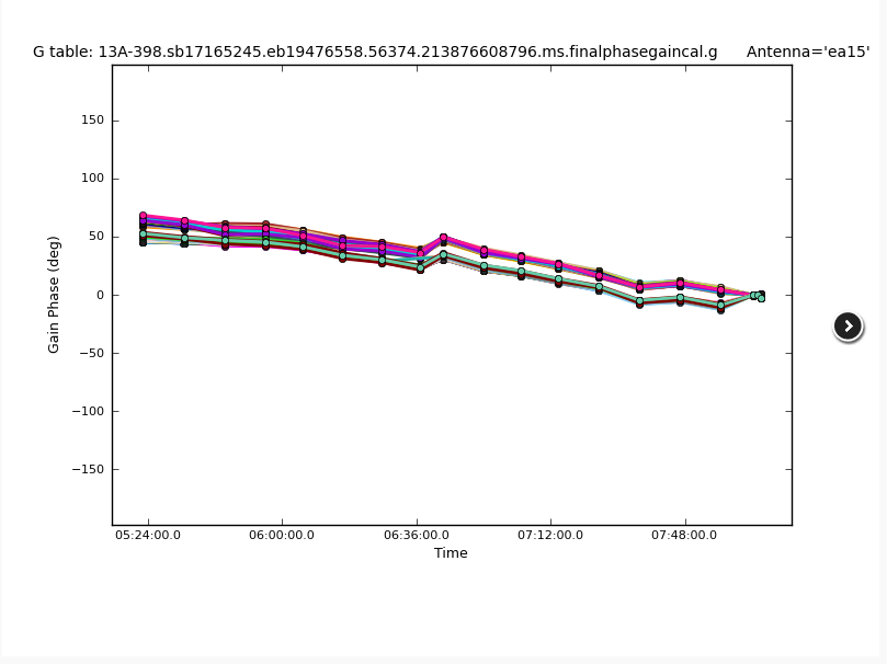 |
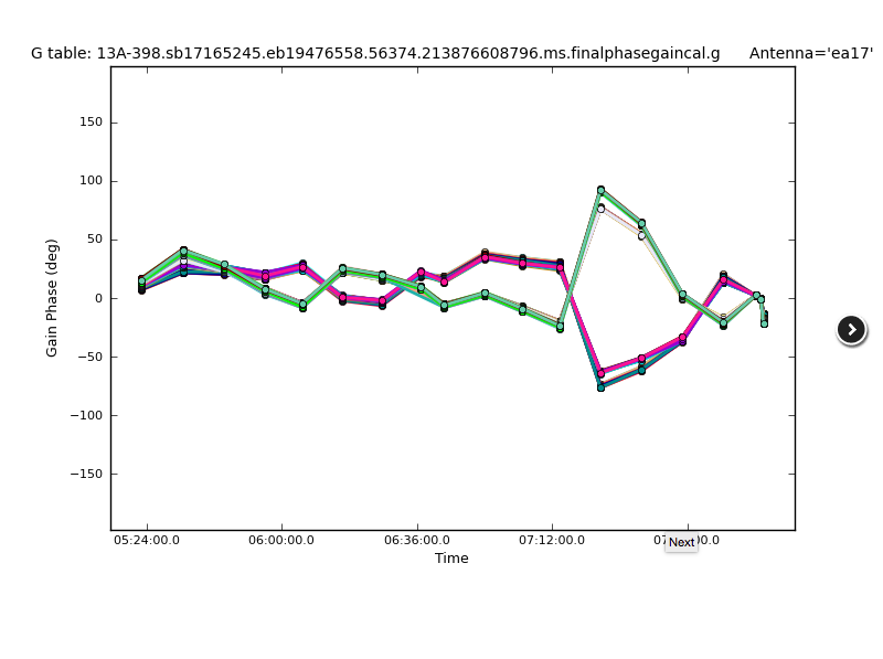 |
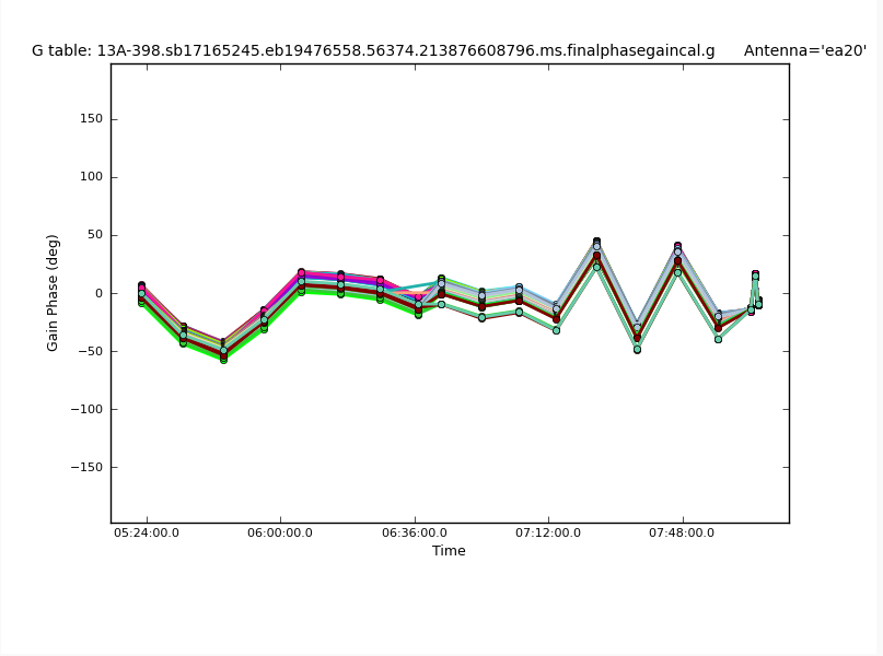 |
CHECK for: strong RFI and whether it was eliminated in later flagging stages or not (especially via a comparison with the output plots of task 14). Also check for jumps in phase and/or amplitude away from spectral window edges. If there are phase jumps for all but the reference antenna, maybe a different choice for the reference antenna should be considered. Also watch out for extreme delays of tens of ns and for very noisy data.

Note that carefully checking calibrator tables in this stage is of particular importance as they are the final tables that are applied to the target source. Phase (and gain) calibration solutions should be inspected in their temporal variations to be smooth and consistent for each calibrator.
Stage 15. hifv_applycals: Apply calibrations from context
The calibration itself now concludes with the application of the derived calibration tables to the entire dataset. That includes all calibrators as well as the target sources. Note that there is no system temperature weighting of the calibration tables for the VLA (calwt=F) since the switched power calibration is currently not used.
In Fig. 30, we show the results of this step. The first table lists the calibration tables that are applied, the fields, spectral windows, and antennas that are calibrated (although note that the spw 0 and 1 are only used for pointing scans and are not calibrated, despite them being listed here). The second table provides information on the flagging statistics. Failed calibration solutions result in flagged calibrator table entries and eventually the data will also be flagged as no calibration can be derived for such data. The following plots show the data of different calibrator sources and spectral windows in different combinations of phase and amplitude against frequency and uv-distance. To start with, the amplitude and phase as a function of frequency are plotted for each baseband of the complex gain/phase calibrator. Next, the amplitudes as a function of uv-distance are plotted for each spw of the flux density calibrator. They are followed by amplitude/time plots for all sources. Finally the amplitudes and phases against time and amplitude against frequency are plotted for each target source baseband.
 |
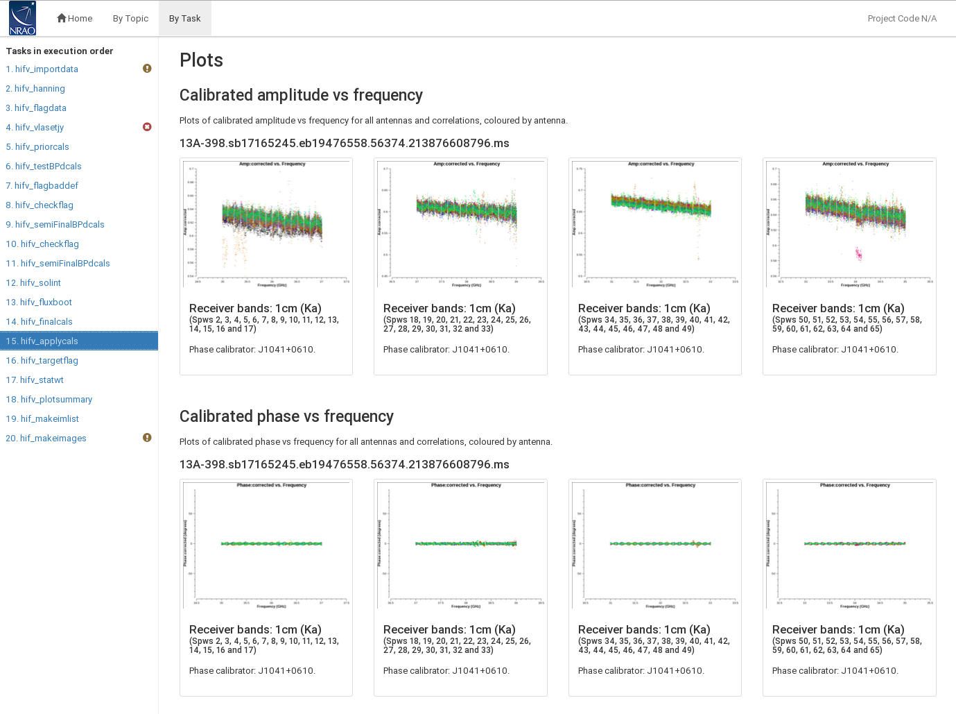 |
 |
 |
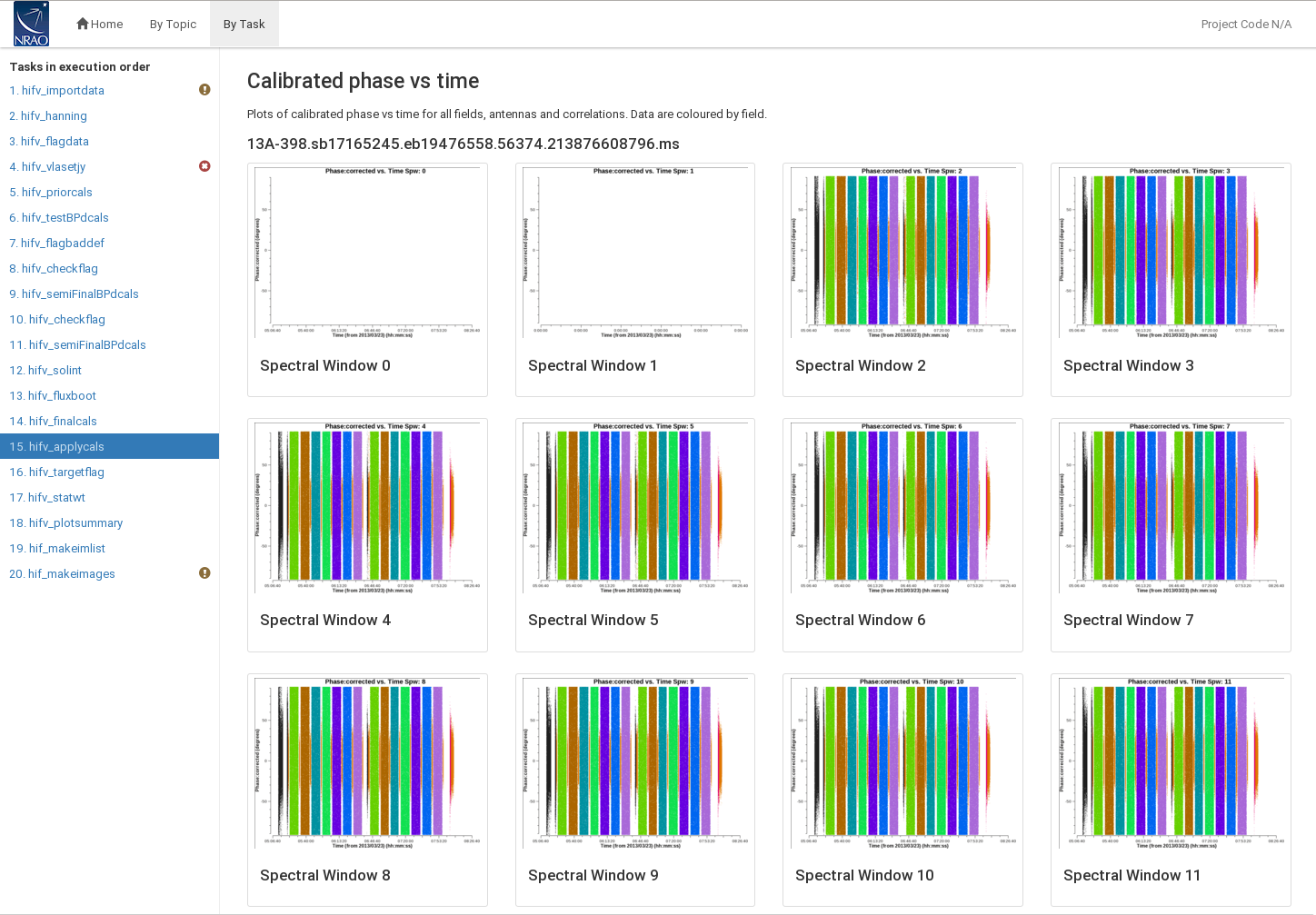 |
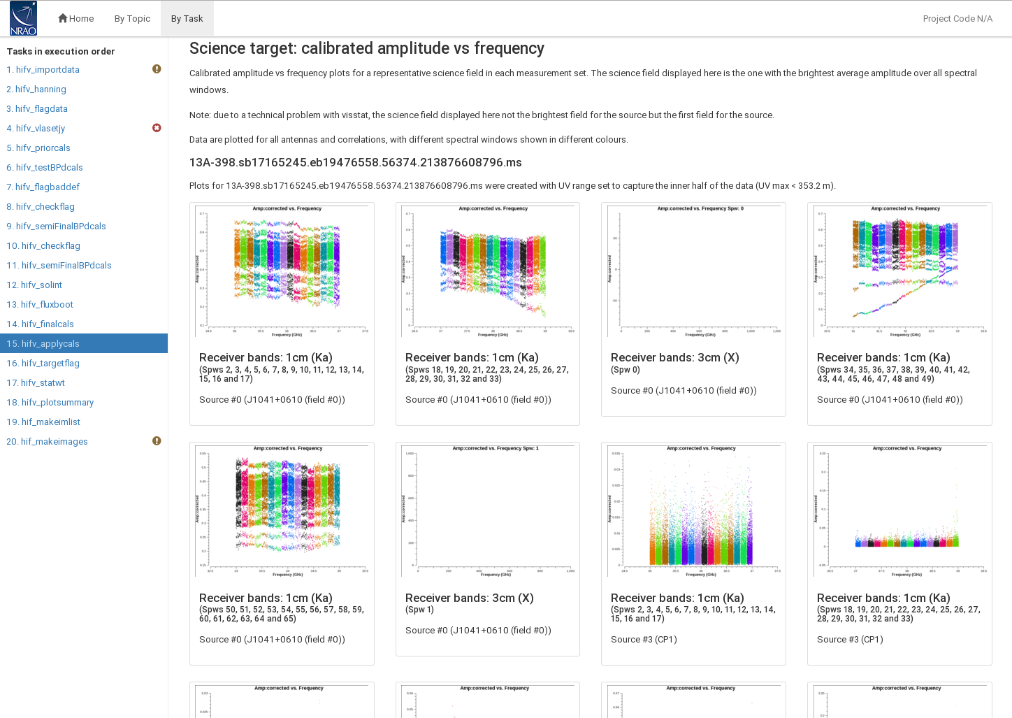 |
 |
 |
In Fig. 31 we show a few examples. a) A spectral window that drops in the calibrated spectrum indicates that it is mis-calibrated. b) Although the phases are well calibrated, residual delays are still visible. The zig-zag pattern is due to a small mismatch in the delay measurement timing (also known as 'delay clunking'). This is an internally generated effect. Typically the effect is averaged out over time. c) Amplitude versus uv-distance plot for the flux density calibrator should should indicate if there is any resolved source structure and the total flux density at the shortest uv-distance. The structure should be similar to the models that are delivered with CASA and that have been attached to the MS with setjy. The offset may indicate one antenna or one time to be offset from the others. This should be inspected further. d) Amplitude versus time for spw=24 shows some increase in noise around 6:00 and also for the red scan near the end. Both should be inspected. e) Amplitude versus frequency for a calibrator shows a baseline or time that has a different slope and offset than the rest and may need to be flagged. For the target source (e) the data is usually noisy and systematic issues are difficult to identify.
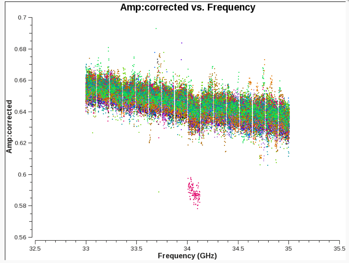 |
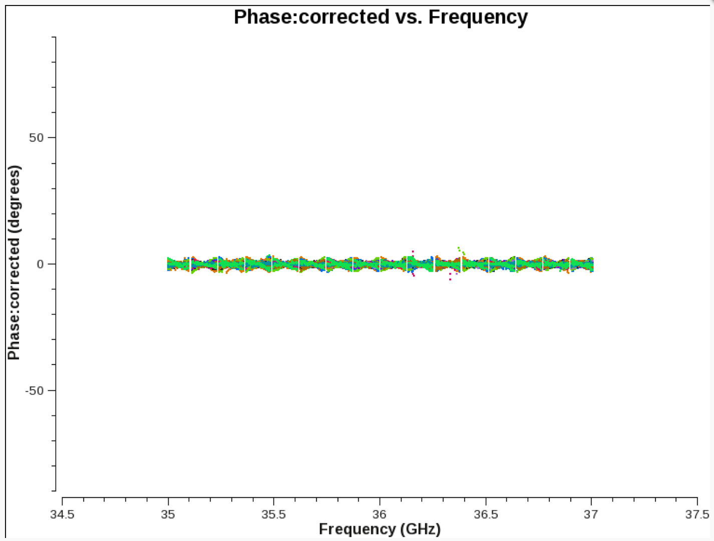 |
 |
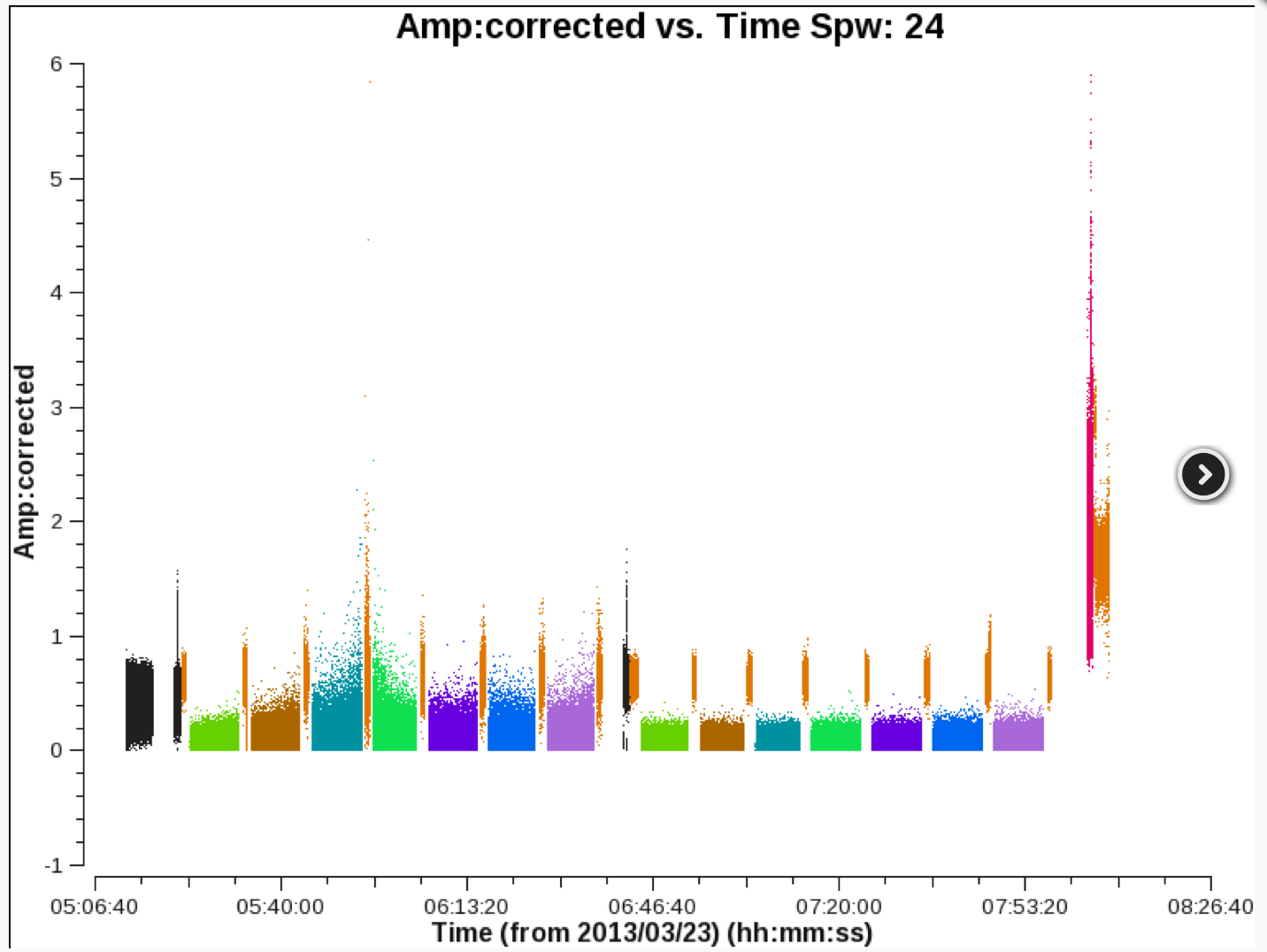 |
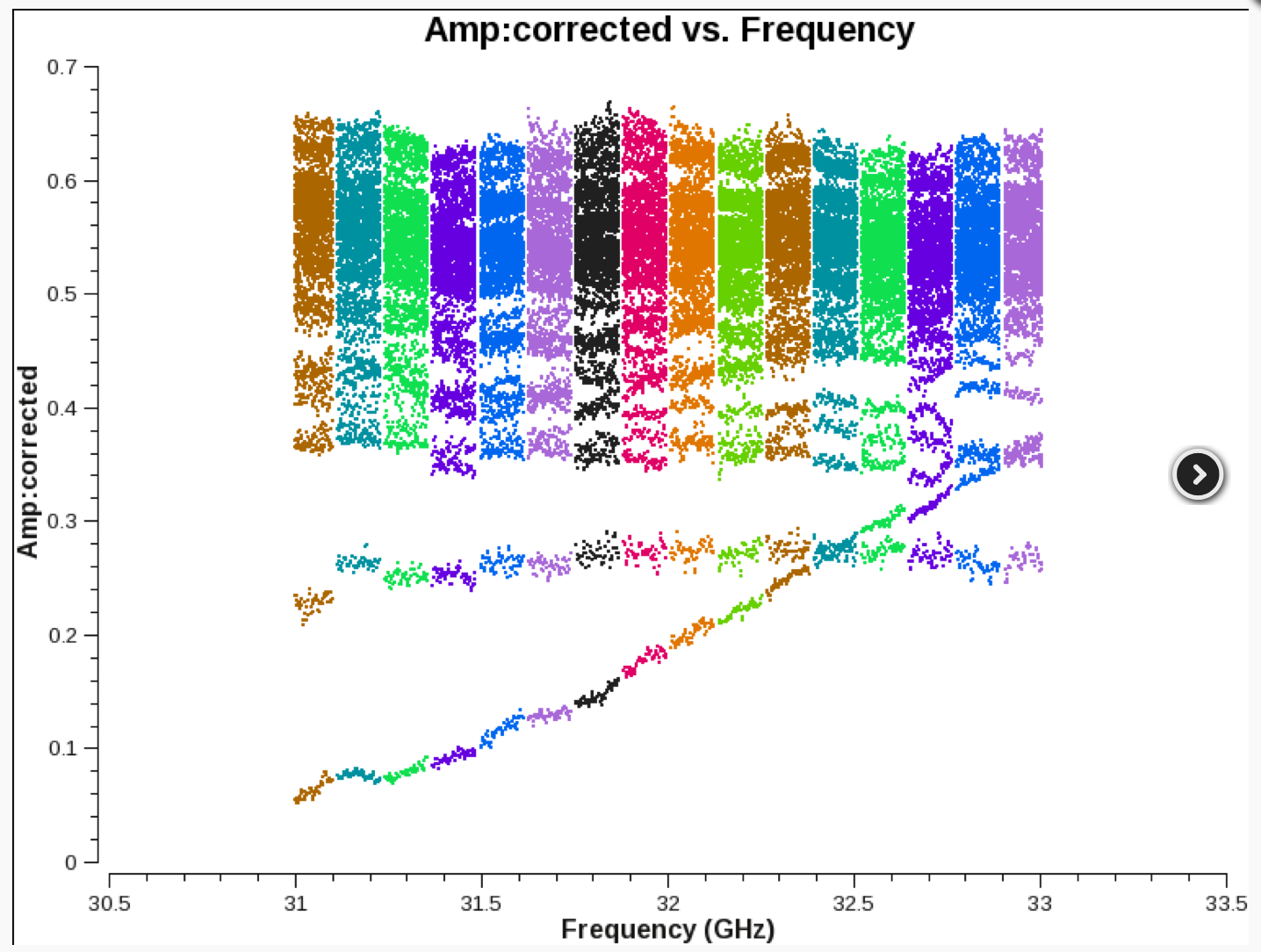 |
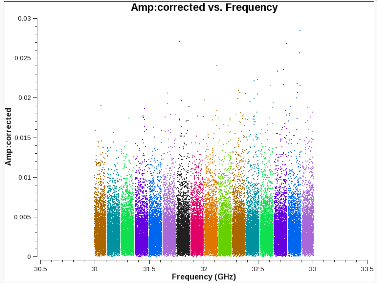 |
CHECK for: a smooth amplitude versus frequency plot. Jumps may indicate mis-calibrated bandpass flux densities for a spectral window.

Also the corrected amplitude of of any calibrator source in each spectral window should be linear in shape and reflect the spectral index in its slope. Check for deviations from a flat amplitude versus uv-distance plot after the model was applied as it could indicate badly calibrated times or antennas.
Stage 16. hifv_targetflag: Targetflag
After the calibration tables are applied, the flagdata automated flagging routine rflag is run one more time on all sources to remove RFI and other outliers from the data.
CHECK for: RFI removal in the target data (use {{plotms}}). Although flagging is performed for all fields, the calibration is applied in a previous stage and any additional flags have no more influence on the calibration tables. Flagging may, however, improve all images that are made in the following stages. In particular the target fields are flagged here for the first time which will benefit their image quality. FOR SPECTRAL LINE DATA: do not run this step as spectral lines may be removed, too (see also below).
Stage 17. hifv_statwt: Reweight visibilities
Since the VLA pipeline is currently not using the switched power calibration, there can be some sensitivity variations of the data over time due to changes in opacity, elevation, temperature (gradients) of the antennas, etc. So it is usually advisable to weigh the data according to the inverse of their noise. This is done via the CASA task statwt and will increase the signal-to noise ratio of images. Note that features such as RFI spikes and spectral lines will influence RMS calculations and usually result in down-weighting data that includes such features.
CHECK for: there is no obvious diagnostic plot for this step but images that are created later should improve in their signal-to-noise. FOR SPECTRAL LINE DATA: do not run this step as spectral lines may be weighted down (see also below).
Stage 18. hifv_plotsummary: VLA Plot Summary
This task produces diagnostic plots of the final, calibrated data. This includes phase as a function of time for all calibrators, as well as amplitude against uv-distance for each calibrator and target field.
Fig. 32 shows that the calibration around 6:00 and 6:30 is still somewhat noisy and additional flagging of the calibrators may be required. Field 12 looks as expected. One may want to check why some values in field 0 are very low and others in field 11 are quite high. Those could correspond to individual antennas, spectral windows, or polarizations. Again, some editing may be required and the pipeline restarted.
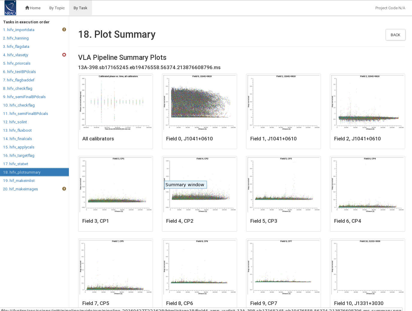 |
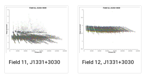 |
CHECK for: outliers, jumps, offsets, and excessive noise.
Stage 19. hif_makeimlist: Compile a list of cleaned images to be calculated
Finally, diagnostic images are made for each spectral window (spw) of the phase and bandpass calibrators (calibrator selection is based on their intents; note that in our case the fallback of the bandpass calibration to use the flux density calibrator scans will not produce an image). The images and basic parameters such as resolution (cell size) and image sizes are listed in this step. The images are available in the directory in which the pipeline was executed (usually where the SDM is located). At this time, images are produced for each spw using the multi-frequency synthesis algorithm, i.e. in continuum mode corrected for spectral dependencies using the stretched uv-coverage as sampled by the observed channel frequencies
In Fig. 33 the images are listed with 0.31" cell/pixel size and 300 pixels on each side. Names and phase centers are given for each spectral window.
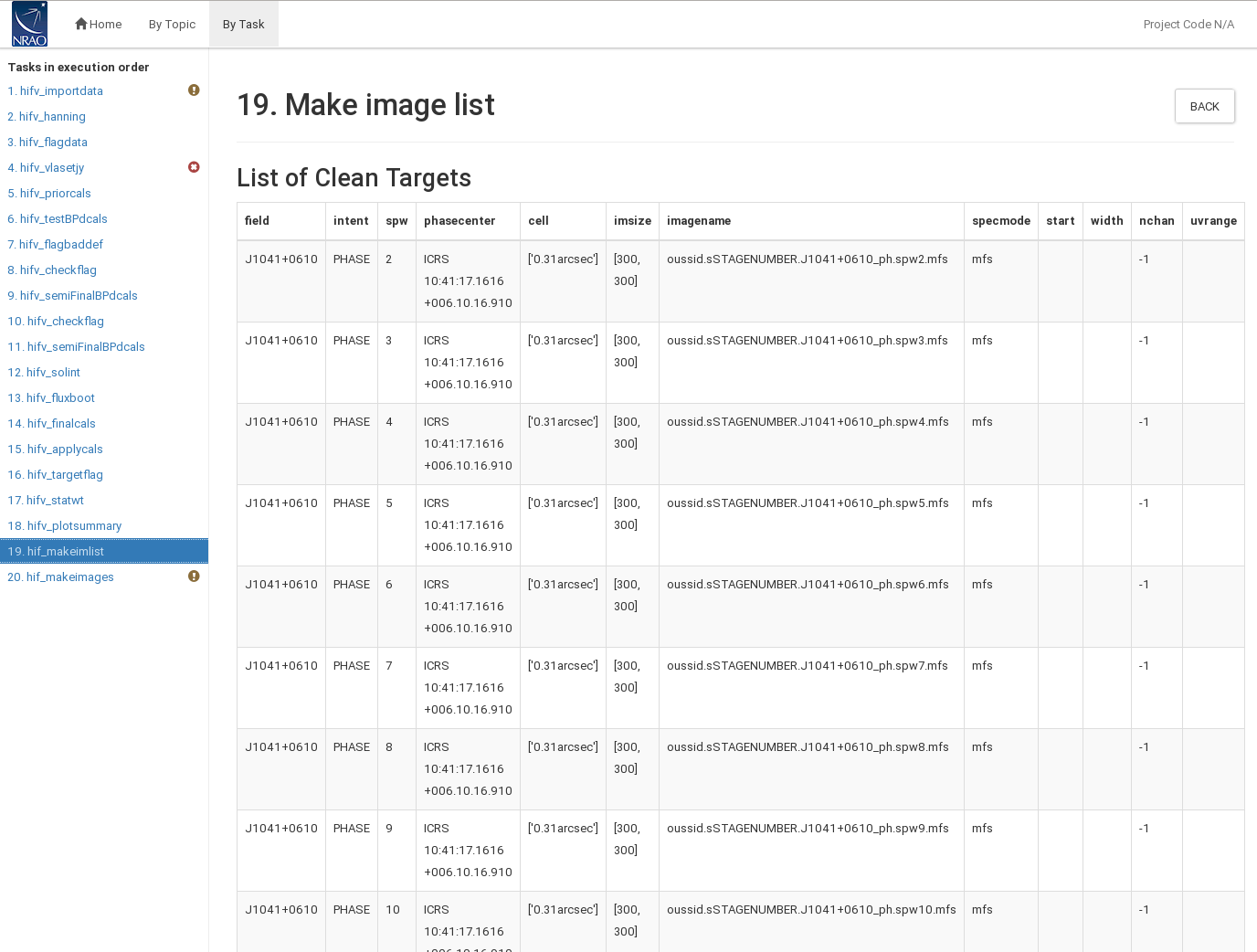 |
CHECK for: appropriate cell size for the images.
Stage 20. hif_makeimages: Calculate clean products
The images from the previous stage are shown in the final pipeline task.
Imaging parameters are provided for each image (Fig. 34). They contain beam characteristics as well as image statistics. A comparison with the theoretical noise is also provided, which are noise values that are based on bandwidth and integration time for typical VLA array parameters (via the radiometer equation). As mentioned earlier, the quality score is not fully implemented in this version of the pipeline and should be ignored.
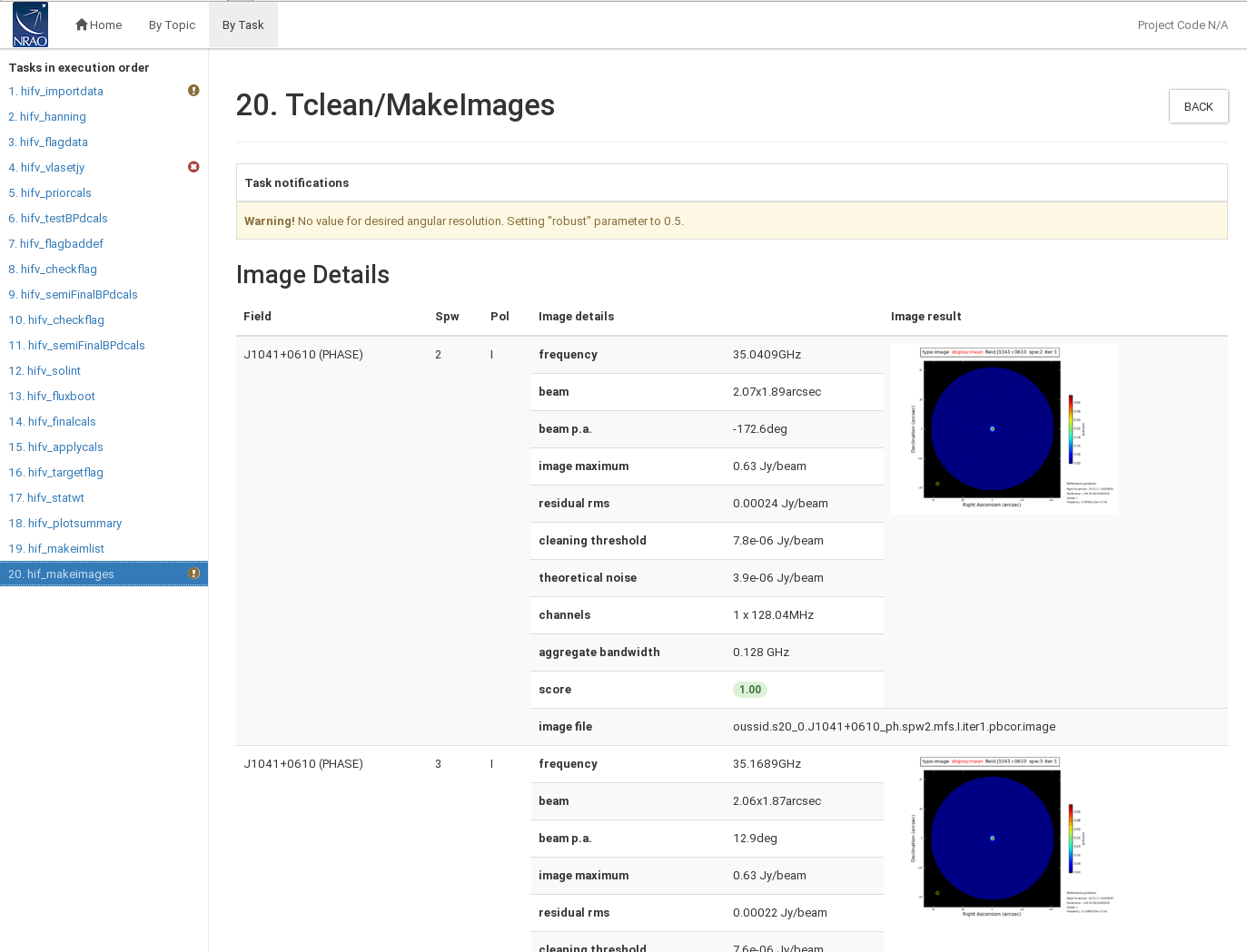 |
CHECK for: degraded images, strong ripples, calibrators that do not resemble the point spread function (psf). Such images may indicate RFI or mis-calibrated sources. If the actual rms is far from the theoretical noise, this could indicate that deeper cleaning is required. But that may not be important for these calibrator images.
Re-Execution of the Pipeline after Flagging
Above we allude to many cases where additional flagging might be required. After manually applying additional flagging (e.g., using flagdata, plotms, viewer/msview or other methods), the pipeline can be re-executed for improved solutions. One should turn off Hanning smoothing for all re-executions given that the data were already Hanning-smoothed and that flags will be slightly extended by smoothing an already flagged MS. Use 'casa_pipescript.py' for re-execution via execfile('casa_pipescript.py') after commenting out 'hifv_hanning' in the 'casa_pipescript.py' file (see below for a similar example).
By default, the pipeline will always revert all flags back to their original state that are saved in the MeasurementSet.flagversions file. It will thus ignore all modifications that were made afterwards.
To avoid resetting all flags, one should manually flag the MeasurementSet and place it in a new directory. Do NOT copy over the related MeasurementSet.flagversions directory. Then run the pipeline with the flagged MS for input to hifv.hifv(['MeasuerementSet']). In that case, the pipeline will not be able to recover original flags and will proceed with the manual flags that the user has applied.
Re-Applying Pipeline Results
Pipeline calibration tables can be re-applied to raw data following the description given on the VLA pipeline webage.
Spectral Line Data
The pipeline is not optimized for calibrating spectral line data. Some pipeline steps may be detrimental for spectral line setups and need to be turned off. The calibrators also require enough signal-to-noise to reliably derive bandpass, gains, phases, etc for the likely more narrow spectral line subbands. The pipeline will also flag edge channels for each spectral window. If the spectral line happens to be located on spectral window (spw) edges, additional modifications to the script may be necessary.
As mentioned above, the following pipeline steps may not be advisable for spectral line data:
Stage 2: hifv_hanning: Hanning smoothing lessens the Gibbs ringing from strong spectral features, usually strong, narrow RFI, or very strong spectral lines such as masers. Hanning smoothing, however, reduces the spectral resolution. Therefore, depending on the data and the science case, one may or may not choose to apply Hanning smoothing. Below we show how to disable the application of Hanning-smoothing in the pipeline if such smoothing is not needed or desired.
Stage 16. hifv_targetflag: Previous flagging was only applied to the calibrator scans. But Stage 16 attempts to auto-flag all fields including target fields. The rflag mode in flagdata is designed to remove outliers that deviate from deviate from a mean level. Strong spectral lines can fulfill this criterion and be flagged. This step should therefore be turned off, too. We recommend manual flagging or a flagdata rflag run that excludes spectral ranges with lines. This step, however, needs to be performed manually after the spectral line pipeline execution.
Stage 17. hifv_statwt: A similar argument applies to the statwt step, where the visibilities are weighted by the inverse of their rms. Strong spectral lines will increase the rms and will therefore be down-weighted. As this is not desired, the step should be turned off and be run manually afterwards, tuned to exclude the spectral line frequency range from the weight calculations.
Given the above, the casa_pipescript.py may be modified as follows. The SDM name (here: '13A-398.sb17165245.eb19476558.56374.213876608796') and maybe other parameters will have to be adapted for the run:
__rethrow_casa_exceptions = True
h_init()
 try:
    hifv_importdata(ocorr_mode='co', vis=['13A-398.sb17165245.eb19476558.56374.213876608796'], createmms='automatic', asis='Receiver CalAtmosphere', overwrite=True)
 #   hifv_hanning(pipelinemode="automatic")
    hifv_flagdata(intents='*POINTING*,*FOCUS*,*ATMOSPHERE*,*SIDEBAND_RATIO*, *UNKNOWN*, *SYSTEM_CONFIGURATION*, *UNSPECIFIED#UNSPECIFIED*', flagbackup=False, scan=True, baseband=True, clip=True, autocorr=True, hm_tbuff='1.5int', template=False, online=True, tbuff=0.0, fracspw=0.05, shadow=True, quack=True, edgespw=True)
    hifv_vlasetjy(fluxdensity=-1, scalebychan=True, reffreq='1GHz', spix=0)
    hifv_priorcals(pipelinemode="automatic")
    hifv_testBPdcals(pipelinemode="automatic")
    hifv_flagbaddef(pipelinemode="automatic")
    hifv_checkflag(pipelinemode="automatic")
    hifv_semiFinalBPdcals(pipelinemode="automatic")
    hifv_checkflag(checkflagmode='semi')
    hifv_semiFinalBPdcals(pipelinemode="automatic")
    hifv_solint(pipelinemode="automatic")
    hifv_fluxboot(pipelinemode="automatic")
    hifv_finalcals(pipelinemode="automatic")
    hifv_applycals(pipelinemode="automatic")
 #   hifv_targetflag(pipelinemode="automatic")
 #   hifv_statwt(pipelinemode="automatic")
    hifv_plotsummary(pipelinemode="automatic")
    hif_makeimlist(nchan=-1, calmaxpix=300, intent='PHASE,BANDPASS')
    hif_makeimages(masklimit=4, noise='1.0Jy', subcontms=False, target_list={}, parallel='automatic', maxncleans=1, weighting='briggs', tlimit=2.0, robust=-999.0, npixels=0)
finally:
    h_save()
We commented out stages 2, 16 and 17. If a spectral line happens to be close to the edge channels, one can decide to turn off edge channel flagging by adding the parameter edgespw=False to all calls of hifv_flagdata.
Once all modifications are made, run the pipeline as:
# In CASA
execfile('casa_pipescript.py')
After the calibration has been obtained, we can now follow up with the flagdata rflag and statwt stages. To start with, we need to define a spw range that contains no lines. Let's assume spw='*:4~180;215~509' is such a range (a line would be in every spw in channels 181 to 214). With this restriction the flagdata task can be run as follows:
# In CASA
flagdata(vis='13A-398.sb17165245.eb19476558.56374.213876608796.ms',
         mode='rflag',spw='*:4~180;215~509',mode='apply')
The spw selection criteria will result in flagging in the line-free part of the spectrum only.
In this example, the statwt command following flagdata would be:
# In CASA
statwt(vis='13A-398.sb17165245.eb19476558.56374.213876608796.ms',
       fitspw='*:4~180;215~509')
where fitspw selects the portion of data that is used for the weight calculation. Again, we use the line-free part of the spectrum.
Mixed Correlator Setups
If data were obtained in mixed correlator modes, the different parts (e.g., spectral line and continuum, or different frequency bands) should be separated first and then the individual parts can be calibrated via the default pipeline or by executing modified casa_pipescript.py files. To start with, we recommend to import the SDM to an MS by applying online flags at the same time. For our SDM, the corresponding CASA command would look like:
# In CASA
importasdm(asdm="13A-398.sb17165245.eb19476558.56374.213876608796",
           vis="13A398.sb17165245.eb19476558.56374.213876608796.ms",
           ocorr_mode="co", applyflags=True, savecmds=True, tbuff=1.5,
           outfile="13A-398.sb17165245.eb19476558.56374.213876608796_flagonline.txt")
Note that we apply the online flags via applyflags=True but still save the flag commands in an outfile in case one would like to inspect those. We set tbuff=1.5 to extend the flags to 1.5 times the integration time (which the pipeline would do in hifv_flagdata).
After that step, use the CASA command split to separate the individual parts of the data to be processed separately. Modify casa_pipescript.py and use each new separate MS as input.
Polarization Calibration
At this stage, the VLA pipeline does not derive and apply polarization calibration. The user may decide to add polarization calibration steps after the pipeline was run by using the pipeline calibration tables as pre-calibration tables as required.
Polarization calibration steps are explained in the respective section of the 3C391 tutorial (in particular the D-term and crosshand delay calibration will be required). We also refer to the corresponding chapter in the CASA Reference Manual and Cookbook.
Weak Calibrators
The VLA pipeline requires a minimum signal-to-noise of ~3 for each spw (each channel for the bandpass) and calibrator scan. If this criterion is not met, the pipeline will likely fail. We are currently implementing additional heuristics to deal with weak calibration sources. This code will be available in upcoming versions of the VLA pipeline.
Correcting Scan Intents
Scan intents should be set up correctly in the OPT before submitting the schedule block for observation.
When incorrect scan intents are identified after observations, the SDM can be modified and updated with new scan intents. The SDM metadata is structured in the form of an XML and can be manually edited. Great care, however, should be taken not to corrupt the structure of the SDM/xml.
To do so, cd into the SDM and edit the file Scan.xml. We strongly recommend making a backup copy of the Scan.xml file in case the edits corrupt the metadata.
Scan.xml is divided into individual <row></row> blocks that identify each scan.
E.g., the first scan in our dataset is listed like:
   <row>
       <scanNumber>1</scanNumber>
       <startTime>4870732142800000000</startTime>
       <endTime>4870732322300000256</endTime>
       <numIntent>1</numIntent>
       <numSubscan>1</numSubscan>
       <scanIntent>1 1 OBSERVE_TARGET</scanIntent>
       <calDataType>1 1 NONE</calDataType>
       <calibrationOnLine>1 1 false</calibrationOnLine>
       <sourceName>J1041+0610</sourceName>
       <flagRow>false</flagRow>
       <execBlockId>ExecBlock_0</execBlockId>
   </row>
We can now change the scan intent, e.g., from OBSERVE_TARGET to CALIBRATE_AMPLI by simply updating the <scanIntent> tag:
   <row>
       <scanNumber>1</scanNumber>
       <startTime>4870732142800000000</startTime>
       <endTime>4870732322300000256</endTime>
       <numIntent>1</numIntent>
       <numSubscan>1</numSubscan>
       <scanIntent>1 1 CALIBRATE_AMPLI</scanIntent>
       <calDataType>1 1 NONE</calDataType>
       <calibrationOnLine>1 1 false</calibrationOnLine>
       <sourceName>J1041+0610</sourceName>
       <flagRow>false</flagRow>
       <execBlockId>ExecBlock_0</execBlockId>
   </row>
If we want to add a second intent, we will have to make additional changes. Let's add CALIBRATE_PHASE:
   <row>
       <scanNumber>1</scanNumber>
       <startTime>4870732142800000000</startTime>
       <endTime>4870732322300000256</endTime>
       <numIntent>2</numIntent>
       <numSubscan>1</numSubscan>
       <scanIntent>1 2 CALIBRATE_AMPLI CALIBRATE_PHASE</scanIntent>
       <calDataType>1 2 NONE NONE</calDataType>
       <calibrationOnLine>1 2 false false</calibrationOnLine>
       <sourceName>J1041+0610</sourceName>
       <flagRow>false</flagRow>
       <execBlockId>ExecBlock_0</execBlockId>
   </row>
Inside <scanIntent> we added the second intent, but also increased the second number from 1 to 2. In addition, we specified <numIntent> to be 2, and added a second entry to <calDataType> and <calibrationOnLine>. For the latter two, we also updated the second number from 1 to 2.
Analoguously, if we now add a third intent, CALIBRATE_BANPDASS, to the same scan, the <row> will look like:
   <row>
       <scanNumber>1</scanNumber>
       <startTime>4870732142800000000</startTime>
       <endTime>4870732322300000256</endTime>
       <numIntent>3</numIntent>
       <numSubscan>1</numSubscan>
       <scanIntent>1 3 CALIBRATE_AMPLI CALIBRATE_PHASE CALIBRATE_BANDPASS</scanIntent>
       <calDataType>1 3 NONE NONE NONE</calDataType>
       <calibrationOnLine>1 3 false false false</calibrationOnLine>
       <sourceName>J1041+0610</sourceName>
       <flagRow>false</flagRow>
       <execBlockId>ExecBlock_0</execBlockId>
   </row>
Check with listobs on the imported MS (after executing importasdm or importevla) if the scan intents are now displayed correctly.
Valid intents are (see SDM definition document):
CALIBRATE_AMPLI : Amplitude calibration scan
CALIBRATE_PHASE : Phase calibration scan
CALIBRATE_BANDPASS : Bandpass calibration scan
CALIBRATE_DELAY : Delay calibration scan
CALIBRATE_FLUX : flux measurement scan.
CALIBRATE_POINTING : Pointing calibration scan
CALIBRATE_POLARIZATION : Polarization calibration scan
CALIBRATE_POL_LEAKAGE :
CALIBRATE_POL_ANGLE :
OBSERVE_TARGET : Target source scan
CALIBRATE_ATMOSPHERE : Atmosphere calibration scan
CALIBRATE_FOCUS : Focus calibration scan. Z coordinate to be derived
CALIBRATE_FOCUS X : Focus calibration scan; X focus coordinate to be derived
CALIBRATE_FOCUS Y : Focus calibration scan; Y focus coordinate to be derived
CALIBRATE_SIDEBAND_RATIO : measure relative gains of sidebands.
CALIBRATE_WVR : Data from the water vapor radiometers (and correlation data) are used to derive their calibration parameters.
DO_SKYDIP : Skydip calibration scan
MAP_ANTENNA_SURFACE : Holography calibration scan
MAP_PRIMARY_BEAM : Data on a celestial calibration source are used to derive a map of the primary beam.
TEST : used for development.
UNSPECIFIED : Unspecified scan intent
CALIBRATE_ANTENNA_POSITION : Requested by EVLA.
CALIBRATE_ANTENNA_PHASE : Requested by EVLA.
MEASURE_RFI : Requested by EVLA.
CALIBRATE_ANTENNA_POINTING_MODEL : Requested by EVLA.
SYSTEM_CONFIGURATION : Requested by EVLA.
CALIBRATE_APPPHASE_ACTIVE : Calculate and apply phasing solutions. Applicable at ALMA.
CALIBRATE APPPHASE PASSIVE : Apply previously obtained phasing solutions. Applicable at ALMA.
OBSERVE_CHECK_SOURCE
Revert back to the original Scan.xml if the above was not successful and contact the NRAO helpdesk for advice.
Scripted Pipeline
In addition to the pipeline that is delivered with CASA, one can also use the VLA scripted pipeline. More modifications are possible to the scripted pipeline and it can be altered to work in almost any circumstance. We refer to the VLA scripted Pipeline webpage for details.
Last checked on CASA Version 4.5.3