Guide To Processing ALMA Data for Cycle 0: Difference between revisions
| (102 intermediate revisions by 4 users not shown) | |||
| Line 1: | Line 1: | ||
== About this Guide, and Cycle 0 ALMA Data == | == About this Guide, and Cycle 0 ALMA Data == | ||
This guide describes steps | This guide describes steps you can take to make science-ready images from Cycle 0 ALMA data available from the ALMA data archive. We begin with the process of locating and downloading the data from the public archive. | ||
This guide is explicitly written for Cycle 0 data. Data for Cycle 1 and beyond will be delivered in a different format and will be described in a separate guide. | This guide is explicitly written for Cycle 0 data. Data for Cycle 1 and beyond will be delivered in a different format and will be described in a separate guide. | ||
For Cycle 0, ALMA data is delivered | For Cycle 0, ALMA data is delivered as a "data package" that includes a set of calibrated data files and a sample of reference images. The data were calibrated and imaged by an ALMA scientist at one of the ALMA Regional Centers (ARCs) using CASA. The scientist developed CASA scripts to complete the calibration and imaging. Cycle 0 data packages also include fully calibrated data sets. Most users will start with these calibrated data and proceed directly to the imaging steps. In many cases where a target is observed with high signal-to-noise, the imaging can be improved dramatically with "self-calibration" on the science target. Self-calibration is the process of using the detected signal in the target source, itself, to tune the phase (and perhaps amplitude) calibrations, as a function of time. | ||
Typically, users interested in making science-ready images with Cycle 0 data from the ALMA archive will take the following steps: | Typically, users interested in making science-ready images with Cycle 0 data from the ALMA archive will take the following steps: | ||
| Line 20: | Line 16: | ||
# Generate moment maps and other analysis products | # Generate moment maps and other analysis products | ||
Most users will not need to modify the calibration supplied in the data package. But in some cases, users may wish to review the calibration steps in detail, make modifications to the calibration scripts, and generate new calibrated data sets. | |||
| Line 35: | Line 31: | ||
Each spectral window covers 234.375 MHz in bandwidth, and the raw data contain 3840 channels, spaced by 61 kHz. Information on the spectral configuration and targets observed must be gleaned from the data themselves. In CASA, you can explore the contents of a data set using the '''listobs''' command. | Each spectral window covers 234.375 MHz in bandwidth, and the raw data contain 3840 channels, spaced by 61 kHz. Information on the spectral configuration and targets observed must be gleaned from the data themselves. In CASA, you can explore the contents of a data set using the '''listobs''' command. | ||
This project was completed by executing a scheduling block three times, leading to three measurement sets. These measurement sets have identical configurations. Our strategy will be to concatenate the three data sets into a single measurement set, and than image that one, combined data set. | |||
=== What other data sets are available? === | === What other data sets are available? === | ||
A [https://almascience.nrao.edu/alma-data/archive/delivery-list Delivery List] of publicly available data sets is provided on the ALMA Science Portal, in the "Data" tab. | A [https://almascience.nrao.edu/alma-data/archive/archive-documentation/delivery-list Delivery List] of publicly available data sets is provided on the ALMA Science Portal, in the "Data" tab. | ||
== Prerequisites : Computing Requirements == | == Prerequisites : Computing Requirements == | ||
ALMA data sets can be very large and require significant computing resources for efficient processing. | ALMA data sets can be very large and require significant computing resources for efficient processing. This example begins with a download of 176 GB of data. For a recommendation on computing resources needed to process ALMA data, check [http://casa.nrao.edu/casa_hardware-requirements.shtml here]. Those who do not have sufficient computing power may wish to arrange a visit to one of the ARCs to use the computing facilities at these sites. To arrange a visit to an ARC, submit a ticket to the [https://help.almascience.org/ ALMA Helpdesk]. Remote use of ARC computing facilities is not available at this time. | ||
== Getting the Data: The ALMA Data Archive == | == Getting the Data: The ALMA Data Archive == | ||
| Line 51: | Line 49: | ||
* [http://almascience.nao.ac.jp/alma-data/archive East Asia] | * [http://almascience.nao.ac.jp/alma-data/archive East Asia] | ||
[[Image:Archive_interface.png|thumb|<caption>The interface to the ALMA data archive.</caption>]] | [[Image:Archive_interface.png|thumb|<caption>'''Fig. 1.''' The interface to the ALMA data archive.</caption>]] | ||
Upon entry into the ALMA Archive Query page, set the "Results View" option to "project" (see the red highlight #1 in Figure 1) and specify the Project Code to 2011.0.00340.S (red highlight #2). Note, if you leave the "Results View" set to "raw data", you will be presented with three rows of data sets in the results page. These correspond to three executions of the observing script. In fact, for Cycle 0 data these rows contains copies of the same data set, so use care not to download the (large!) data set three times. By setting "Results View" to "project", you see just one entry, and that is the one you'd like to download. | Upon entry into the ALMA Archive Query page, set the "Results View" option to "project" (see the red highlight #1 in Figure 1) and specify the Project Code to 2011.0.00340.S (red highlight #2). Note, if you leave the "Results View" set to "raw data", you will be presented with three rows of data sets in the results page. These correspond to three executions of the observing script. In fact, for Cycle 0 data these rows contains copies of the same data set, so use care not to download the (large!) data set three times. By setting "Results View" to "project", you see just one entry, and that is the one you'd like to download. | ||
| Line 77: | Line 75: | ||
== Overview of Delivered Data and Products == | == Overview of Delivered Data and Products == | ||
To get to the | To get to the directory that contains the data package, do: | ||
<source lang="bash"> | <source lang="bash"> | ||
| Line 92: | Line 90: | ||
</source> | </source> | ||
These directories are standard for all cycle 0 data | These directories are standard for all cycle 0 data packages. The README file describes the files in the distribution and includes notes from the ALMA scientist who performed the initial calibration and imaging. | ||
In our example, the directories contain the following files: | In our example, the directories contain the following files: | ||
| Line 157: | Line 155: | ||
== What if I need to redo the Calibration? == | == What if I need to redo the Calibration? == | ||
In most cases, users should not need to redo the calibration. However, you should consult [https://help.almascience.org/ | In most cases, users should not need to redo the [[Guide_To_Processing_ALMA_DataGlossary#Calibration|calibration]]. However, you should consult [https://help.almascience.org/kb/articles/will-re-reduction-improve-the-cycle-0-data-products-provided-by-the-archive this knowledgebase article] for suggestions on instances when recalibration may be beneficial. You might also want to redo calibration to include your own preferences (for flagging, gain solutions calculation, flux references), or to tailor it to your specific needs. If you would like to learn how to redo calibration, proceed to the [[Guide_To_Redo_Calibration_For_ALMA_Cycle_0|Guide To Redo Calibration For ALMA Cycle 0]]. | ||
<span id="DataConcatenation"></span> | |||
< | |||
</ | |||
== Data Concatenation == | == Data Concatenation == | ||
| Line 205: | Line 182: | ||
== Imaging == | == Imaging == | ||
A first step is to list the contents of the '''calibarated.ms''' measurement set. | A first step is to list the contents of the '''calibarated.ms''' measurement set using the CASA task {{listobs}}. | ||
<source lang="python"> | <source lang="python"> | ||
| Line 212: | Line 189: | ||
</source> | </source> | ||
The text file '''calibrated.listobs''' now contains a summary of the contents of this data file. The listobs output includes the following section: | The text file '''calibrated.listobs''' now contains a summary of the contents of this data file. The {{listobs}} output includes the following section: | ||
Spectral Windows: (4 unique spectral windows and 1 unique polarization setups) | Spectral Windows: (4 unique spectral windows and 1 unique polarization setups) | ||
| Line 223: | Line 200: | ||
We see that the data file contains 4 spectral windows. The H2D+ data are contained in SpwID=0 (rest frequency of H2D+: 372.42138 GHz) and the N2H+ data are contained in SpwID=1 (rest frequency of N2H+: 372.67249 GHz). Note that the Ch0 column gives the sky frequency at channel 0. To get central frequencies for the spectral windows, add 117.1875 MHz for Spectral Window IDs 0 and 1. Subtract 117.1875 MHz for IDs 2 and 3. (Note the channel width for these IDs is negative, indicating the frequencies increase in the opposite direction as SpwID 0 and 1. | We see that the data file contains 4 spectral windows. The H2D+ data are contained in SpwID=0 (rest frequency of H2D+: 372.42138 GHz) and the N2H+ data are contained in SpwID=1 (rest frequency of N2H+: 372.67249 GHz). Note that the Ch0 column gives the sky frequency at channel 0. To get central frequencies for the spectral windows, add 117.1875 MHz for Spectral Window IDs 0 and 1. Subtract 117.1875 MHz for IDs 2 and 3. (Note the channel width for these IDs is negative, indicating the frequencies increase in the opposite direction as SpwID 0 and 1. | ||
Our strategy will be to image and self-calibrate the continuum data first. We will then apply the self-cal solutions to each of the two line data files, and image those second. In general terms, we will follow the steps | Our strategy will be to image and self-calibrate the continuum data first. We will then apply the self-cal solutions to each of the two line data files, and image those second. In general terms, we will follow the steps outlined in the [[TWHydraBand7_Imaging_4.2|Science Verification CASAguide on TW Hya]]. You can also refer to the '''ScriptForImaging.py''' script included with the data package. | ||
Other data sets may require different strategies. This strategy works best in this case because the continuum is bright, and suitable for self-calibration. A data set with a bright line may benefit from self-calibration on the line, instead of the continuum. | Other data sets may require different strategies. This strategy works best in this case because the continuum is bright, and suitable for self-calibration. A data set with a bright line may benefit from self-calibration on the line, instead of the continuum. | ||
| Line 229: | Line 206: | ||
=== Continuum Imaging === | === Continuum Imaging === | ||
First we will split off the TW Hya data and average the data over 100 channels, eliminating a few channels at each edge prior to averaging. This will generate a data set suitable for continuum imaging. The final data set has 6.1 MHz channels, sufficient to allow efficient cleaning with the "Multi-Frequency Synthesis" algorithm used by the CASA task | First we will split off the TW Hya data and average the data over 100 channels, eliminating a few channels at each edge prior to averaging. This will generate a data set suitable for continuum imaging. The final data set has 6.1 MHz channels, sufficient to allow efficient cleaning with the "Multi-Frequency Synthesis" algorithm used by the CASA task {{clean}}. | ||
<source lang="python"> | <source lang="python"> | ||
# In CASA | # In CASA | ||
split(vis='calibrated.ms', outputvis='TWHya_cont.ms', datacolumn='data', keepflags= | split(vis='calibrated.ms', outputvis='TWHya_cont.ms', datacolumn='data', keepflags=True, field='TW Hya', spw='0~3:21~3820', width=100) | ||
listobs(vis='TWHya_cont.ms', listfile='TWHya_cont.listobs') | listobs(vis='TWHya_cont.ms', listfile='TWHya_cont.listobs') | ||
</source> | </source> | ||
Now plot amplitude vs. channel with | Now plot amplitude vs. channel with {{plotms}} to see what needs to be flagged. See Figure 2. | ||
<source lang="python"> | <source lang="python"> | ||
# In CASA | # In CASA | ||
plotms(vis='TWHya_cont.ms',spw='0~3',xaxis='channel',yaxis='amp', | plotms(vis='TWHya_cont.ms',spw='0~3',xaxis='channel',yaxis='amp', | ||
avgtime='1e8',avgscan= | avgtime='1e8',avgscan=True,coloraxis='spw',iteraxis='spw',xselfscale=True) | ||
</source> | </source> | ||
We flag the line emission as follows: | [[Image:Plotms_amp.png|thumb|<caption>'''Fig. 2.''' In SpwID = 1 we notice elevated amplitudes in channel 24. This arises from the strong N2H+ line emission. We'd like to flag this channel prior to imaging the continuum.</caption>]] | ||
We flag the line emission using the {{flagdata}} task as follows: | |||
<source lang="python"> | <source lang="python"> | ||
| Line 256: | Line 233: | ||
</source> | </source> | ||
Next we will generate a first-pass continuum image. | Next we will generate a first-pass continuum image. We will use mode "mfs" to generate a single continuum image from all the data. | ||
<source lang="python"> | <source lang="python"> | ||
| Line 267: | Line 244: | ||
mode = 'mfs', | mode = 'mfs', | ||
imagermode = 'csclean', | imagermode = 'csclean', | ||
interactive = | interactive=True, | ||
imsize = [300, 300], | imsize = [300, 300], | ||
cell = '0.1arcsec', | cell = '0.1arcsec', | ||
| Line 274: | Line 251: | ||
robust = 0.5) | robust = 0.5) | ||
</source> | </source> | ||
[[Image:Cont_clean1.png|thumb|<caption>'''Fig. 3.''' After a few minutes, the '''clean''' procedure returns a plot of the dirty map as shown.</caption>]] | |||
Note that at ~370 GHz the ALMA primary beam has a width of ~ 20 arcseconds FWHM. We want to image an area at least as large as that. Also, for this data set the synthesized beam is about 0.49 x 0.46 arcseconds. We have selected a cell size of 0.1 arcsec to fully sample the synthesized beam. | Note that at ~370 GHz the ALMA primary beam has a width of ~ 20 arcseconds FWHM. We want to image an area at least as large as that. Also, for this data set the synthesized beam is about 0.49 x 0.46 arcseconds. We have selected a cell size of 0.1 arcsec to fully sample the synthesized beam. | ||
| Line 279: | Line 260: | ||
We'd like to do some cleaning to achieve our best image. In {{clean}}, the multifrequency synthesis mode grids each spectral channel independently. Since the uv-spacing is a function of frequency, this will actually achieve greater uv-coverage than if all the channels and spectral windows had been averaged in advance. | We'd like to do some cleaning to achieve our best image. In {{clean}}, the multifrequency synthesis mode grids each spectral channel independently. Since the uv-spacing is a function of frequency, this will actually achieve greater uv-coverage than if all the channels and spectral windows had been averaged in advance. | ||
Our initial cleaned model will be used as the image model in the next self-calibration step. It is essential that only "real" signal be included in the image model, so we will clean the image conservatively. We set '''interactive= | Our initial cleaned model will be used as the image model in the next self-calibration step. It is essential that only "real" signal be included in the image model, so we will clean the image conservatively. We set '''interactive=True''' to make the clean mask interactively. This also allows us to stop cleaning when the signal from the source starts to approach the surrounding "noise" areas in the residual map. | ||
Once the Clean Viewer opens, click on the ellipse tool with your left mouse button, and draw a circle around the continuum emission with the left mouse button. Double click inside the region with the left mouse button when you are happy with it. It will turn from green to white when the clean mask is accepted. To begin the clean use the green arrow in the "Next action" section on the Viewer Display GUI. | Once the Clean Viewer opens, click on the ellipse tool with your left mouse button, and draw a circle around the continuum emission with the left mouse button. Double click inside the region with the left mouse button when you are happy with it. It will turn from green to white when the clean mask is accepted. To begin the clean use the green arrow in the "Next action" section on the Viewer Display GUI. | ||
| Line 295: | Line 272: | ||
</pre> | </pre> | ||
You should | You should choose the green circle arrow. It will clean 100 iterations (as shown in the GUI) and then show the residual image. If necessary you can adjust the color scale to examine the residuals more clearly. The middle mouse button is initially assigned to the "plus" icon, which adjusts the color scale. Also, note in the logger that {{clean}} reports the clean flux recovered so far, the min/max residuals, and the synthesized beam size. | ||
In this example we will clean 500 iterations by clicking the green arrow five times, without changing the clean mask. After this we have cleaned about 1.5 Jy and we have residuals of about 5-7 mJy. Click the red and white "X" icon to conclude the cleaning process. | In this example we will clean 500 iterations by clicking the green arrow five times, without changing the clean mask. After this we have cleaned about 1.5 Jy and we have residuals of about 5-7 mJy. Click the red and white "X" icon to conclude the cleaning process. | ||
There are a few points to note: | There are a few points to note: | ||
* Real emission will not get | * Real emission will not get cleaned if you do not put a clean box on it. | ||
* Conversely, if you put a clean box on a region that contains no real emission and clean deeply, you can amplify that | * Conversely, if you put a clean box on a region that contains no real emission and clean deeply, you can amplify any artifacts or features in that region. | ||
* Thus, it's best to be conservative. Stop cleaning when the residuals inside the clean box approach those outside it. Start with a small clean box surrounding what is clearly real emission, and add to it after some iterations, if necessary. You can generally see fainter "real" features in the residuals. | * Thus, it's best to be conservative. Stop cleaning when the residuals inside the clean box approach those outside it. Start with a small clean box surrounding what is clearly real emission, and add to it after some iterations, if necessary. You can generally see fainter "real" features in the residuals. | ||
* | * There is no default mask. So if you start an interactive clean and do not make a mask, the algorithm will clean nothing. | ||
{{clean}} will generate several files: | {{clean}} will generate several files: | ||
| Line 322: | Line 299: | ||
=== First cycle of self-calibration: phase only === | === First cycle of self-calibration: phase only === | ||
Next we can use the clean model to self-calibrate the uv-data. The process of self-calibration tries to adjust the data to better match the model you give it. That is why it is important to make the model as good as you can. {{clean}} places a uv-model of the resulting image in the file <tt>TWHydra_cont.model</tt>. This model can then be used to self-calibrate the data using {{gaincal}}. We use '''gaintype='T'''' to tell it to average the polarizations before deriving phase solutions (to improve sensitivity by a factor of sqrt(2)). The "solution interval" ('''solint''') is critical and may require some experimentation to get optimal results. From {{listobs}} we see that the integration time of these data is 6.05 seconds, so we want to select a solution interval that is at least this long, and is matched to the expected coherence time of the atmosphere, while maintaining adequate S/N. We can use '''solint=30s''' as a starting point. It is often best to start with a larger '''solint''' and then work your way down to the integration time if the S/N of the data permits. For the reasons described in the [[TWHydraBand7_Calibration_4.2]] tutorial, we want to determine the phases before tackling amplitudes. Se we set '''calmode='p''''. | Next we can use the clean model to self-calibrate the uv-data. The process of self-calibration tries to adjust the data to better match the model you give it. That is why it is important to make the model as good as you can. {{clean}} places a uv-model of the resulting image in the file <tt>TWHydra_cont.model</tt>. This model can then be used to self-calibrate the data using {{gaincal}}. We use '''gaintype='T'''' to tell it to average the polarizations before deriving phase solutions (to improve sensitivity by a factor of sqrt(2)). The "solution interval" ('''solint''') is critical and may require some experimentation to get optimal results. From {{listobs}} we see that the integration time of these data is 6.05 seconds, so we want to select a solution interval that is at least this long, and is matched to the expected coherence time of the atmosphere, while maintaining adequate S/N. We can use '''solint=30s''' as a starting point. It is often best to start with a larger '''solint''' and then work your way down to the integration time if the S/N of the data permits. For the reasons described in the [[TWHydraBand7_Calibration_4.2|TW Hydra Science Verification]] tutorial, we want to determine the phases before tackling amplitudes. Se we set '''calmode='p''''. | ||
<source lang="python"> | <source lang="python"> | ||
| Line 332: | Line 309: | ||
</source> | </source> | ||
[[Image:C0Guide_self_1_phase.png|thumb|<caption>'''Fig. 4.''' Phase solutions from self_1.pcal with solint=30s.</caption>]] | |||
Next we'll examine the solutions using | We are using '''combine=' '''' to get independent solutions for each spw. If the S/N is insufficient to get independent solutions, you can try combining spectral windows with '''combine='spw''''. We have plenty of S/N in these data so we keep them separate. | ||
Next we'll examine the solutions using {{plotcal}}. | |||
<source lang="python"> | <source lang="python"> | ||
# In CASA | # In CASA | ||
| Line 347: | Line 323: | ||
</source> | </source> | ||
The magnitude of corrections gives you a sense of | The magnitude of the corrections here gives you a sense of the accuracy of the phase transfer from the calibrators. Check that the phases are being well tracked by the solutions, i.e. smoothly varying functions of time within a given scan. Also the solutions for each spectral window should be nearly identical, indicating that the phase offsets between spectral windows are well calibrated already. In this example, the solutions look fine, overall. If they didn't you could try increasing the solint and/or combining the spw into a single solution. | ||
When you are happy with the solutions, apply them with {{applycal}} | |||
<source lang="python"> | <source lang="python"> | ||
# In CASA | # In CASA | ||
applycal(vis='TWHya_cont.ms',field='',gaintable=['self_1.pcal'],calwt= | applycal(vis='TWHya_cont.ms',field='',gaintable=['self_1.pcal'],calwt=False) | ||
</source> | </source> | ||
Next clean the source again | [[Image:Viewer_pcal1.png|thumb|<caption>'''Fig. 5.''' Clean residuals after 500 iterations and the 1st phase only self-cal. Residuals inside mask are higher than the "noise" outside.</caption>]] | ||
Next clean the source again. To save time we can start with the clean mask from the last iteration. If you make interactive adjustments to the clean mask, they will be written to the new mask '''TWHydra.continuum.1pcal.mask''', and not the old one. | |||
<source lang="python"> | <source lang="python"> | ||
| Line 370: | Line 346: | ||
weighting='briggs',robust=0.5, | weighting='briggs',robust=0.5, | ||
mask='TWHya.continuum.mask',usescratch=False, | mask='TWHya.continuum.mask',usescratch=False, | ||
interactive= | interactive=True,threshold='1mJy',niter=10000) | ||
</source> | </source> | ||
Now after the first 500 iterations you see that the residuals inside the clean mask are higher than last time. This is because flux that had been spread out in the map due to poorly correlated phases has been | Now after the first 500 iterations you see that the residuals inside the clean mask are higher than last time. This is because flux that had been spread out in the map due to poorly correlated phases has been recovered in the source, thereby increasing its flux. Let's continue cleaning for 1200 iterations. | ||
Now let's compare the maps made before and after self-calibration using {{imview}}. | Now let's compare the maps made before and after self-calibration using {{imview}}. | ||
| Line 383: | Line 359: | ||
</source> | </source> | ||
Once the Viewer Display panel opens, click on the box next in the "Images" panel and then use the | Once the Viewer Display panel opens, click on the box next in the "Images" panel and then use the tape deck buttons in the panel to alternate between the two images. We use the '''range''' parameter to put the two images on the same color scale. It is obvious that the self-calibrated image has much better residuals. To quantify the improvement in rms noise, use the rectangle tool to draw a region that excludes the central source and then double click inside. Repeat that process for the second image. Statistics for the region will print to the terminal: | ||
<pre style="background-color: #fffacd;"> | <pre style="background-color: #fffacd;"> | ||
| Line 410: | Line 386: | ||
The self-calibrated image has improved the rms noise by a factor of 5. | The self-calibrated image has improved the rms noise by a factor of 5. | ||
=== Second cycle of self-calibration: phase only === | |||
Now that we have a better model, we can try to determine phase solutions again using a second round of phase-only self calibration. We will write the gain solutions to a new table, but these solutions will replace the solutions we determined in the first round. It may be useful to experiment with the solution interval. Keep in mind that the integration time is 6.05 seconds for this observation. (The integration time we refer to here is the "dump time" of the correlator, not the cumulative on-source time.) | Now that we have a better model, we can try to determine phase solutions again using a second round of phase-only self calibration. We will write the gain solutions to a new table, but these solutions will replace the solutions we determined in the first round. It may be useful to experiment with the solution interval. Keep in mind that the integration time is 6.05 seconds for this observation. (The integration time we refer to here is the "dump time" of the correlator, not the cumulative on-source time.) | ||
| Line 437: | Line 413: | ||
<source lang="python"> | <source lang="python"> | ||
# In CASA | # In CASA | ||
applycal(vis='TWHya_cont.ms',field='',gaintable=['self_2.pcal'],calwt= | applycal(vis='TWHya_cont.ms',field='',gaintable=['self_2.pcal'],calwt=False) | ||
</source> | </source> | ||
Note, here, that applycal applies the gain solutions to the raw data and overwrites any results in the "corrected data" column of the measurement set, so this calibration replaces what we applied after the first-round solutions. | Note, here, that {{applycal}} applies the gain solutions to the raw data and overwrites any results in the "corrected data" column of the measurement set, so this calibration replaces what we applied after the first-round solutions. | ||
Now clean again, updating '''mask''' with the most recent mask file. | Now clean again, updating '''mask''' with the most recent mask file. | ||
| Line 452: | Line 428: | ||
weighting='briggs',robust=0.5,usescratch=False, | weighting='briggs',robust=0.5,usescratch=False, | ||
mask='TWHya.continuum.1pcal.mask', | mask='TWHya.continuum.1pcal.mask', | ||
interactive= | interactive=True,threshold='1mJy',niter=10000) | ||
</source> | </source> | ||
Clean again, interactively. In general, you should pay attention to the total flux being cleaned after each round, and the residuals inside the clean box as compared to those outside. When the cleaned flux is small and the residuals match, the image has been sufficiently cleaned. Stop by hitting the red X on the GUI. In this case, let's again clean for 1200 iterations. The task reports a total cleaned flux and residuals similar to what we saw after the first round of cleaning: | Clean again, interactively. In general, you should pay attention to the total flux being cleaned after each round, and the residuals inside the clean box as compared to those outside. When the cleaned flux in the latest round is small and the residuals inside the clean box match those outside it, the image has been sufficiently cleaned. Stop by hitting the red X on the GUI. In this case, let's again clean for 1200 iterations. The task reports a total cleaned flux and residuals similar to what we saw after the first round of cleaning: | ||
<pre style="background-color: #fffacd;"> | <pre style="background-color: #fffacd;"> | ||
| Line 493: | Line 469: | ||
</pre> | </pre> | ||
This small improvement suggests that we have | This small improvement suggests that we have reached an end point with phase-only self-cal. | ||
=== Third cycle of self-calibration: amplitude & phase === | |||
Next we will add amplitude self-calibration to the process. Amplitude changes more slowly than phase, so we will determine one solution per scan. We can set '''solint = 'inf'''', which tells {{gaincal}} to use the "combine" parameter to determine how to set the solution interval. With "combine" set to the default ('''combine = ''''') we will get one solution per scan. | |||
Also, note that we set "gaintable" to 'self_2.pcal'. This tells {{gaincal}} to apply the former phase-only solutions prior to determining the new amplitude+phase solutions. So, the new solutions will be incremental. Later when we apply these solutions to the data sets, we must be sure to apply both the phase-only solutions and the amplitude+phase solutions. | |||
[[Image:C0Guide_self_ap_phase.png|thumb|<caption>'''Fig. 6.''' Incremental phase solutions after the third round of self-calibration.</caption>]] | |||
[[Image:C0Guide_self_ap_amp.png|thumb|<caption>'''Fig. 7.''' Amplitude solutions after the third round of self-calibration.</caption>]] | |||
[[Image: | |||
<source lang="python"> | <source lang="python"> | ||
| Line 526: | Line 501: | ||
</source> | </source> | ||
Use the "next" button on the plotcal GUI to advance the plot to see additional antennas. Since phase corrections have already been applied, we see that the new incremental phase solutions are fairly small. The amplitude corrections are at the level of ~10% in many cases, but there is considerable variance among different antennas. | Use the "next" button on the {{plotcal}} GUI to advance the plot to see additional antennas. Since phase corrections have already been applied, we see that the new incremental phase solutions are fairly small. The amplitude corrections are at the level of ~10% in many cases, but there is considerable variance among different antennas. See Figures 6 and 7 for the phase and amplitude solutions. | ||
We can apply the calibration now with | We can apply the calibration now with {{applycal}}. Note we apply two gain tables. | ||
<source lang="python"> | <source lang="python"> | ||
# In CASA | # In CASA | ||
applycal(vis='TWHya_cont.ms',field='',gaintable=['self_2.pcal','self_ap.cal'],calwt= | applycal(vis='TWHya_cont.ms',field='',gaintable=['self_2.pcal','self_ap.cal'],calwt=False) | ||
</source> | </source> | ||
[[Image:C0Guide_selfcal_time.png|thumb|<caption>'''Fig. 8.''' Amplitudes as a function of time. We see that one of the scans has anomolously high amplitudes and should be flagged.</caption>]] | |||
[[Image: | |||
Let's plot the u,v data against both time and u,v | [[Image:C0Guide_selfcal_uvdist.png|thumb|<caption>'''Fig. 9.''' Amplitudes as a function of u,v distance. The many high amplitudes come from scan 72.</caption>]] | ||
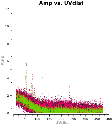
Let's plot the u,v data against both time and u,v distance. It is a good idea to check these after an amplitude self-calbration to be sure that it worked properly. Occasionally, a few spurious bits of data will get wildly incorrect values by the amplitude self-cal. | |||
<source lang="python"> | <source lang="python"> | ||
| Line 556: | Line 530: | ||
</source> | </source> | ||
Using the "locate" tool in the | Figures 8 and 9 show results from the previous two commands. | ||
Using the "locate" tool in the {{plotms}} GUI, select a few bad data points and confirm the scan number. We can see that bad data points exist for, at least, spw 0 and 1. To be conservative, we can flag all of scan 72. It's not much data compared to the full observation. | |||
<source lang="python"> | <source lang="python"> | ||
| Line 563: | Line 539: | ||
</source> | </source> | ||
Replot the u,v data to confirm the bad data have been removed. IMPORTANT: when re-plotting this data set in | Replot the u,v data to confirm the bad data have been removed. IMPORTANT: when re-plotting this data set in {{plotms}}, you must remember to select the "force reload" button on the GUI. Otherwise, the plot will not update with the new flags. | ||
If the plots | If the plots look good, you can proceed to make the final continuum image. | ||
<source lang="python"> | <source lang="python"> | ||
| Line 574: | Line 550: | ||
imsize=300,cell=['0.1arcsec'],spw='', | imsize=300,cell=['0.1arcsec'],spw='', | ||
weighting='briggs',robust=0.5,usescratch=False, | weighting='briggs',robust=0.5,usescratch=False, | ||
interactive= | interactive=True,threshold='0.1mJy',niter=5000,npercycle=1000) | ||
</source> | </source> | ||
[[Image:C0Guide_cont_clean_residuals.png|thumb|<caption>Here we show the residuals plotted in the viewer during the cleaning process. We decided to stop cleaning when the residuals reached the level shown.</caption>]] | [[Image:C0Guide_cont_clean_residuals.png|thumb|<caption>'''Fig. 10.''' Here we show the residuals plotted in the viewer during the cleaning process. We decided to stop cleaning when the residuals reached the level shown.</caption>]] | ||
You will need to execute over a thousand iterations in total to get the image fully cleaned, so we start the clean process with 1000 iterations and press the green circle. In the GUI, you should then adjust the number of iterations per cycle down to 100 for additional cleaning. Update the clean box if necessary, by expanding the region with a larger ellipse. Note that the pattern of residuals inside the clean box may not come to match that outside it, but you want to clean until the magnitude of the residuals is similar, inside it and out. In this case, the cleaning takes about 1500 iterations. | You will need to execute over a thousand iterations in total to get the image fully cleaned, so we start the clean process with 1000 iterations and press the green circle. In the GUI, you should then adjust the number of iterations per cycle down to 100 for additional cleaning. Update the clean box if necessary, by expanding the region with a larger ellipse. Note that the pattern of residuals inside the clean box may not come to match that outside it, but you want to clean until the magnitude of the residuals is similar, inside it and out. In this case, the cleaning takes about 1500 iterations. | ||
The | The {{clean}} task reports a total cleaned flux of 1.76 Jy. | ||
<source lang="python"> | <source lang="python"> | ||
| Line 615: | Line 591: | ||
We see that the amplitude+phase self-cal made a significant improvement in the rms of the image, compared to the phase-only self-cal from 0.41 mJy to 0.24 mJy. | We see that the amplitude+phase self-cal made a significant improvement in the rms of the image, compared to the phase-only self-cal from 0.41 mJy to 0.24 mJy. | ||
== Apply Calibration to the Full Data Set and Split the Line Data == | === Apply Calibration to the Full Data Set and Split the Line Data === | ||
Now we apply the self-calibration derived from the continuum emission to the full-resolution | Now we apply the self-calibration derived from the continuum emission to the full-resolution spectral cube. | ||
<source lang="python"> | <source lang="python"> | ||
# In CASA | # In CASA | ||
applycal(vis='calibrated.ms',gaintable=['self_2.pcal','self_ap.cal'],calwt= | applycal(vis='calibrated.ms',gaintable=['self_2.pcal','self_ap.cal'],calwt=False) | ||
</source> | </source> | ||
| Line 642: | Line 618: | ||
</source> | </source> | ||
== Subtracting the Continuum == | === Subtracting the Continuum === | ||
The next step in the processing is to subtract the continuum from the full data set, in preparation for imaging the line emission. We'll do the subtraction in the u,v plane. | The next step in the processing is to subtract the continuum from the full data set, in preparation for imaging the line emission. We'll do the subtraction in the u,v plane. We determine the continuum from line-free channels, so we begin by plotting the u,v amplitudes using '''plotms''', to identify channels with the N2H+ line. | ||
<source lang="python"> | <source lang="python"> | ||
# In CASA | # In CASA | ||
plotms(vis='TWHydra_N2H+.ms',xaxis='channel',yaxis='amp',avgtime='1e8',avgscan= | plotms(vis='TWHydra_N2H+.ms',xaxis='channel',yaxis='amp',avgtime='1e8',avgscan=True) | ||
</source> | </source> | ||
In this data set, the line emission is evident directly in the u,v amplitudes. | |||
[[Image:C0Guide_N2H+_amp.png|thumb|<caption>'''Fig. 11.''' Here we show the u,v amplitudes from {{plotms}} for the spectral window containing the N2H+ line, which is detected near channel 2440.</caption>]] | |||
In this data set, the line emission is evident directly in the u,v amplitudes. Although the line is not really strong enough to have much impact on continuum subtraction, we will avoid the N2H+ line anyway (good practice) and fit the continuum to the spectrum using line-free channels. In fitting for the continuum we will also avoid a few channels at the band edges, where there can sometimes be erratic data. | |||
<source lang="python"> | <source lang="python"> | ||
| Line 658: | Line 637: | ||
</source> | </source> | ||
It is useful at this stage to determine the velocity range of the detected emission. We'll use this later when we image the line emission. Using the {{plotms}} GUI, set the X axis to "Velocity" and then select the vertical "Trans" tab. Here, set the Frame to "LSRK", the velocity defn to "RADIO", and the Rest Freq to 372672.49 MHz. Then re-plot the data by clicking the "Plot" button. Notice that the emission falls between ~ 2-4 km/s, which is consistent with the known recession velocity of TW Hydra, about 2.9 km/s. | |||
=== Imaging N2H+ === | |||
The final step is to image the N2H+ line emission using the {clean}} task. | |||
Many of the imaging parameters are the same as we used for the continuum, but now we have a few new parameters to set for the spectral cube: '''mode''', '''start''', '''width''', '''nchan''', '''restfreq''', and '''outframe'''. When making spectral images you have three choices for '''mode''': "channel", "velocity", or "frequency". The data are recorded into channels spaced by a constant frequency increment, but for spectral line analysis it's often more useful to have a constant velocity increment. For '''mode='velocity'''', the desired '''start''' and '''width''' also need to be given in velocity units. | |||
ALMA does not do on-line Doppler Tracking and the native frame of the data is topocentric (TOPO). If you do not specify '''outframe''', the output cube will also be in TOPO, which is not very useful for spectral line work. By specifying the '''outframe''' parameter, {{clean}} will make the doppler shift correction. Alternatively it can be done prior to imaging with the {{cvel}} task. | |||
In our example here, we will image the N2H+ line in the range 0-4 km/s using steps of 0.1 km/s. Our choice of velocity increment is determined by the channel spacing. From the {{listobs}} output, we know the channel spacing is 61 kHz, which corresponds to ~ 0.05 km/s at 372 GHz. The true velocity resolution is worse than the channel spacing by about a factor of 2. So, 0.1 km/s steps in velocity is a good choice. | |||
<source lang="python"> | <source lang="python"> | ||
# In CASA | # In CASA | ||
clean(vis = 'TWHydra_N2H+.ms.contsub', imagename = 'line.N2H+', mode = 'velocity', nchan = | os.system('rm -rf line.N2H+.*') | ||
width = '0. | clean(vis = 'TWHydra_N2H+.ms.contsub', imagename = 'line.N2H+', mode = 'velocity', nchan = 40, start = '1.0km/s', | ||
interactive = | width = '0.1km/s', outframe = 'LSRK', restfreq = '372.67249GHz', imagermode = 'csclean', | ||
interactive=True, niter=1000, imsize = [300, 300], cell = '0.1arcsec', weighting = 'briggs', robust = 0.0) | |||
</source> | </source> | ||
Imaging spectral data cubes with complex line emission can be an arduous task. In this case, we use the clean viewer to step through each spectral channel and define a clean mask for each channel individually. This is usually the best approach when the structure is complex and changing from one spectral channel to the next, as it is for the N2H+ line in TW Hydra. For simpler structures, it can be sufficient to define a single clean mask and apply it for all channels. | |||
After the viewer GUI appears, you may wish to maximize the size of the "Display" panel by deselecting the "Cursors" panel, if necessary. Then step through channels with the tape deck controls, and create a clean mask for each channel with detected line emission, as you did for the continuum cleaning. In this case, make sure that the radio button at the top of the GUI has "This Channel" selected, to create a separate mask for each spectral channel. | |||
Click the green arrow to clean with 100 iterations, then click the "play" button on the tape deck to see the residuals, You will see significant residuals remaining in each channel. Continue cleaning until the residuals inside the clean boxes match those outside. If you reach 5000 iterations, the {{clean}} task will end itself (since we specified niter=5000). If you'd like to stop sooner, click the red "X" button. | |||
That's it! You've got a data cube with N2H+ ready for analysis. | |||
Apart from imaging this targeted channel range, it is also important to image the full data cube to explore the full spectral bandwidth observed. A full imaging could be accomplished as follows: | |||
<source lang="python"> | |||
# In CASA | |||
os.system('rm -rf line.N2H+.*') | |||
clean(vis = 'TWHydra_N2H+.ms.contsub', imagename = 'line.N2H+', mode = 'channel', start=0, width=10, imagermode = 'csclean', | |||
interactive=False, niter=0, imsize = [300, 300], cell = '0.1arcsec', weighting = 'briggs', robust = 0.0) | |||
</source> | |||
=== What About the H2D+? === | |||
Recall the first spectral window (spw='0') in the '''calibrated.ms''' data set contains the anticipated H2D+ line emission. Imaging of that line can proceed in much the same manner as we have done for the N2D+ line. In this case, though, there is no obvious detection of the H2D+ line. So we will not repeat the steps in this guide. | |||
== Image Analysis == | |||
[[Image:C0Guide_N2H+_1chan.png|thumb|<caption>'''Fig. 12''' Here we show one spectral channel in the final N2H+ image. The faint purple line marks an elliptical region that we use to determine an integrated spectrum, shown in the next figure.</caption>]] | |||
The CASA viewer offers some powerful capabilities for exploring spectral data cubes. We are currently preparing CASA Guides that discuss '''Using the Viewer to Extract Spectra''', and '''Making Moment Maps'''. Check back later! | |||
Here, we will demonstrate how to make moment maps from the N2H+ data cube. First examine the final image in the viewer: | |||
<source lang="python"> | |||
# In CASA | |||
viewer('line.N2H+.image') | |||
</source> | |||
You should see a result as shown in Figure 12. | |||
[[Image:C0Guide_N2H+_profile.png|thumb|<caption>'''Fig. 13.''' This figure shows a spectrum of N2H+ determined by integrating the flux in each channel over the area marked by the purple ellipse in the previous figure.</caption>]] | |||
Use the ellipse drawing tool to define an elliptical region that encompasses all the line emission, from all channels, and then select "Spectral Profile" from the "Tools" menu to generate a spectrum, as shown in Figure 13 to the right. We are showing the X axis in units of velocity. If we select "channels" from the Spectral Profile GUI, we can see that the line emission extends from channels 11-26. | |||
Now make the Moment 0 map: | |||
<source lang="python"> | |||
# In CASA | |||
os.system('rm -rf line.N2H+.image.mom0') | |||
immoments(imagename='line.N2H+.image',moments=[0], outfile='line.N2H+.image.mom0', chans='11~26') | |||
</source> | |||
<source lang="python"> | |||
# In CASA | |||
os.system('rm -rf ') | |||
os.system('rm -rf ') | |||
immoments(imagename='line.N2H+.image',moments=[1,2], | |||
outfile='line.N2H+.image.mom', | |||
chans='11~26',includepix=[0.1,100]) | |||
</source> | |||
Display all three moment maps in the viewer, overlaid with continuum contours. | |||
<source lang="python"> | |||
# In CASA | |||
imview( raster=[ {'file':'line.N2H+.image.mom0'}, | |||
{'file':'line.N2H+.image.mom.weighted_coord'}, | |||
{'file':'line.N2H+.image.mom.weighted_dispersion_coord'} ], | |||
contour={'file':'TWHya.continuum.apcal.image', 'base':0, 'unit':0.0025, 'levels':[3,100]} ) | |||
</source> | |||
[[Image:C0Guide_3moments.png|thumb|<caption>'''Fig. 14.''' The first three moment images from the N2H+ data cube.</caption>]] | |||
To see all three raster images simultaneously, open the viewer's Panel Display Options (the "P-wrench" icon in the viewer tool bar), click "Number of panels", and change "Number of panels in x" to 3. | |||
Latest revision as of 19:03, 7 September 2023
About this Guide, and Cycle 0 ALMA Data
This guide describes steps you can take to make science-ready images from Cycle 0 ALMA data available from the ALMA data archive. We begin with the process of locating and downloading the data from the public archive.
This guide is explicitly written for Cycle 0 data. Data for Cycle 1 and beyond will be delivered in a different format and will be described in a separate guide.
For Cycle 0, ALMA data is delivered as a "data package" that includes a set of calibrated data files and a sample of reference images. The data were calibrated and imaged by an ALMA scientist at one of the ALMA Regional Centers (ARCs) using CASA. The scientist developed CASA scripts to complete the calibration and imaging. Cycle 0 data packages also include fully calibrated data sets. Most users will start with these calibrated data and proceed directly to the imaging steps. In many cases where a target is observed with high signal-to-noise, the imaging can be improved dramatically with "self-calibration" on the science target. Self-calibration is the process of using the detected signal in the target source, itself, to tune the phase (and perhaps amplitude) calibrations, as a function of time.
Typically, users interested in making science-ready images with Cycle 0 data from the ALMA archive will take the following steps:
- Download the data from the Archive
- Inspect the Quality Assurance plots and data files
- Inspect the reference images supplied with the data package
- Combine the calibrated data sets into a single calibrated measurement set
- Self-calibrate and image the combined data set
- Generate moment maps and other analysis products
Most users will not need to modify the calibration supplied in the data package. But in some cases, users may wish to review the calibration steps in detail, make modifications to the calibration scripts, and generate new calibrated data sets.
About the Sample Data: H2D+ and N2H+ in TW Hya
The data for this example comes from ALMA Project 2011.0.00340.S, "Searching for H2D+ in the disk of TW Hya v1.5", for which the PI is Chunhua Qi. Part of the data for this project has been published in Qi et al. 2013.
This observation has three scientific objectives:
- Image the submm continuum structure in TW Hya
- Image the H2D+ line structure (rest frequency 372.42138 GHz)
- Image the N2H+ line structure (rest frequency 372.67249 GHz)
Eventually we will see that the data is distilled to 4 "spectral windows" used for science. The N2H+ line is in one spectral window, the H2D+ is in another window, and the other two windows contribute to the continuum observation. The best continuum map will be generated from the line-free channels of all 4 spectral windows.
Each spectral window covers 234.375 MHz in bandwidth, and the raw data contain 3840 channels, spaced by 61 kHz. Information on the spectral configuration and targets observed must be gleaned from the data themselves. In CASA, you can explore the contents of a data set using the listobs command.
This project was completed by executing a scheduling block three times, leading to three measurement sets. These measurement sets have identical configurations. Our strategy will be to concatenate the three data sets into a single measurement set, and than image that one, combined data set.
What other data sets are available?
A Delivery List of publicly available data sets is provided on the ALMA Science Portal, in the "Data" tab.
Prerequisites : Computing Requirements
ALMA data sets can be very large and require significant computing resources for efficient processing. This example begins with a download of 176 GB of data. For a recommendation on computing resources needed to process ALMA data, check here. Those who do not have sufficient computing power may wish to arrange a visit to one of the ARCs to use the computing facilities at these sites. To arrange a visit to an ARC, submit a ticket to the ALMA Helpdesk. Remote use of ARC computing facilities is not available at this time.
Getting the Data: The ALMA Data Archive
The ALMA data archive is part of the ALMA Science Portal. A copy of the archive is stored at each of the ARCs, and you can connect to the nearest archive through these links:
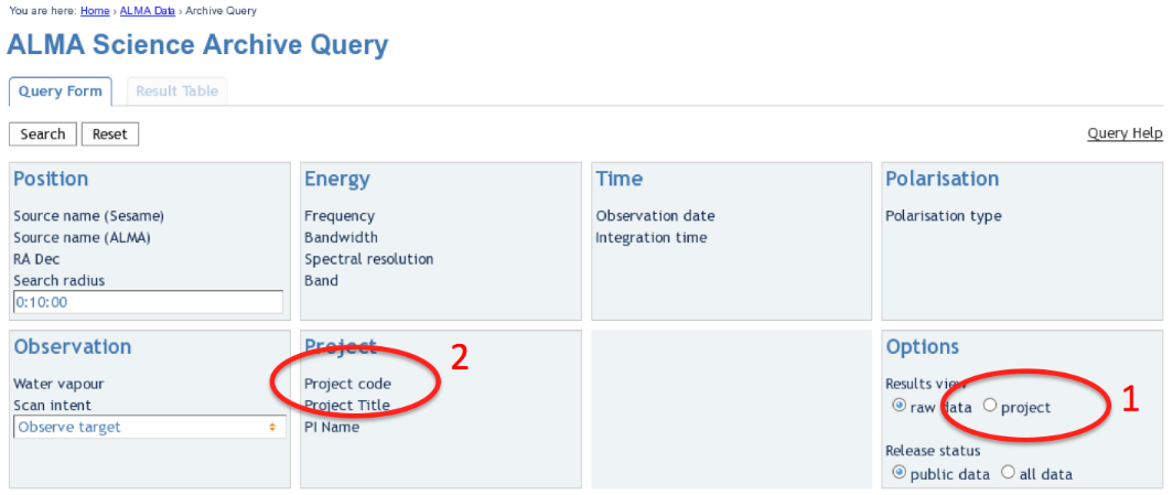
Upon entry into the ALMA Archive Query page, set the "Results View" option to "project" (see the red highlight #1 in Figure 1) and specify the Project Code to 2011.0.00340.S (red highlight #2). Note, if you leave the "Results View" set to "raw data", you will be presented with three rows of data sets in the results page. These correspond to three executions of the observing script. In fact, for Cycle 0 data these rows contains copies of the same data set, so use care not to download the (large!) data set three times. By setting "Results View" to "project", you see just one entry, and that is the one you'd like to download.
You can download the data through the Archive GUI. For more control over the download process, you can use the Unix shell script provided on the Request Handler page. This script has a name like "downloadRequest84998259script.sh". You need to put this file into a directory that contains ample disk space, and execute the script in your shell. For example, in bash:
# In bash
 % chmod +x downloadRequest84998259script.sh
 % ./downloadRequest84998259script.sh
Unpacking the data
The data you have downloaded for this particular project includes 17 tar files. Unpack these using the following command:
# In bash
 % for i in $(ls *.tar); do echo 'Untarring ' $i; tar xvf $i; done
At this point you will have a directory called "2011.0.00340.S" with the full data distribution.
Overview of Delivered Data and Products
To get to the directory that contains the data package, do:
# In bash
 % cd 2011.0.00340.S/sg_ouss_id/group_ouss_id/member_ouss_2012-12-05_id
Here you will find the following entries:
# In bash
 % ls
 calibrated  calibration  log  product  qa  raw  README  script
These directories are standard for all cycle 0 data packages. The README file describes the files in the distribution and includes notes from the ALMA scientist who performed the initial calibration and imaging.
In our example, the directories contain the following files:
-- calibrated/
  |-- uid___A002_X554543_X207.ms.split.cal/
  |-- uid___A002_X554543_X3d0.ms.split.cal/
  |-- uid___A002_X554543_X667.ms.split.cal/
-- calibration/
  |-- uid___A002_X554543_X207.calibration/
  |-- uid___A002_X554543_X207.calibration.plots/
  |-- uid___A002_X554543_X3d0.calibration/
  |-- uid___A002_X554543_X3d0.calibration.plots/
  |-- uid___A002_X554543_X667.calibration/
  |-- uid___A002_X554543_X667.calibration.plots/
-- log/
  |-- uid___A002_X554543_X207.calibration.log
  |-- uid___A002_X554543_X3d0.calibration.log
  |-- uid___A002_X554543_X667.calibration.log
  |-- Imaging.log
  |-- 340.log
-- product/
  |-- TWHya.continuum.fits
  |-- TWHya.N2H+.fits
  |-- TWHya.continuum.mask/
  |-- TWHya.H2D+.mask/
  |-- TWHya.N2H+.mask/
-- qa/
  |-- uid___A002_X554543_X207__textfile.txt
  |-- uid___A002_X554543_X207__qa2_part1.png
  |-- uid___A002_X554543_X207__qa2_part2.png
  |-- uid___A002_X554543_X207__qa2_part3.png
  |-- uid___A002_X554543_X3d0__textfile.txt
  |-- uid___A002_X554543_X3d0__qa2_part1.png
  |-- uid___A002_X554543_X3d0__qa2_part2.png
  |-- uid___A002_X554543_X3d0__qa2_part3.png
  |-- uid___A002_X554543_X667__textfile.txt
  |-- uid___A002_X554543_X667__qa2_part1.png
  |-- uid___A002_X554543_X667__qa2_part2.png
  |-- uid___A002_X554543_X667__qa2_part3.png
-- raw/
  |-- uid___A002_X554543_X207.ms.split/
  |-- uid___A002_X554543_X3d0.ms.split/
  |-- uid___A002_X554543_X667.ms.split/
-- script/
  |-- uid___A002_X554543_X207.ms.scriptForCalibration.py
  |-- uid___A002_X554543_X3d0.ms.scriptForCalibration.py
  |-- uid___A002_X554543_X667.ms.scriptForCalibration.py
  |-- scriptForImaging.py
  |-- import_data.py
  |-- scriptForFluxCalibration.py
- calibrated: This directory contains a calibrated measurement set for each of the execution blocks in the project. In our case, there are three. These could be imaged separately, or combined to make a single calibrated measurement set. In this guide we will combine the three executions prior to imaging.
- calibration: Auxiliary data files generated in the calibration process.
- The "calibration.plots" directories contain (a few hundred) plots generated during the calibration process. These can be useful for the expert user to assess the quality of the calibration at each step.
- log: Log files from the CASA sessions used by the ALMA scientist to calibrate and image the data. These are provided for reference.
- product: The final data products from the calibration and imaging process. The directory contains "reference" images that are used to determine the quality of the observation, but they are not necessarily science-ready. The data files here can used for initial inspections.
- qa: The result of standardized Quality Assessment tests. The data from each scheduling block goes through such a quality assessment, and all data delivered to the public ALMA Archive have passed the quality assessment. It is worthwhile to review the plots and text files contained here. You will find plots of the antenna configuration, UV coverage, calibration results, Tsys, and so on.
- raw: The "raw" data files. If you would like to tune or refine the calibration, these files would be your starting point. In fact, these data files do have certain a priori calibrations already applied, amounting to steps 0-6 of the calibration scripts provided in the data package. These steps include a priori flagging and application of WVR, Tsys, and antenna position corrections.
- script: These are the scripts developed and applied by the ALMA scientist, to calibrate the data and generate reference images. These scripts cannot be applied directly to the raw data provided in this data distribution, but they do serve as a valuable reference to see the steps that need to be taken to re-calibrate the data, if you so choose.
What if I need to redo the Calibration?
In most cases, users should not need to redo the calibration. However, you should consult this knowledgebase article for suggestions on instances when recalibration may be beneficial. You might also want to redo calibration to include your own preferences (for flagging, gain solutions calculation, flux references), or to tailor it to your specific needs. If you would like to learn how to redo calibration, proceed to the Guide To Redo Calibration For ALMA Cycle 0.
Data Concatenation
The data package includes a fully calibrated data set for each of the execution blocks. Each data set has been calibrated first according to the steps in the scriptForCalibration scripts, and subsequently by the steps listed in the scriptForFluxCalibration.py script. The data delivery package does not include a concatenated measurement set, so we will do the concatenation here, then proceed to imaging. Let's make a new directory for imaging, and do all subsequent work from there.
# In bash
 mkdir Imaging
 cd Imaging
 casapy
and then, in CASA:
# In CASA
concat(vis = ['../calibrated/uid___A002_X554543_X207.ms.split.cal', '../calibrated/uid___A002_X554543_X3d0.ms.split.cal',
       '../calibrated/uid___A002_X554543_X667.ms.split.cal'], concatvis = 'calibrated.ms')
This operation could take an hour or longer. When completed, we have created a calibrated measurement set calibrated.ms, which is ready for imaging.
Imaging
A first step is to list the contents of the calibarated.ms measurement set using the CASA task listobs.
# In CASA
listobs(vis='calibrated.ms',listfile='calibrated.listobs')
The text file calibrated.listobs now contains a summary of the contents of this data file. The listobs output includes the following section:
Spectral Windows:  (4 unique spectral windows and 1 unique polarization setups)
 SpwID  Name                           #Chans   Frame   Ch0(MHz)  ChanWid(kHz)  TotBW(kHz) BBC Num  Corrs
 0      ALMA_RB_07#BB_1#SW-01#FULL_RES   3840   TOPO  372286.368        61.035    234375.0       1  XX  YY
 1      ALMA_RB_07#BB_2#SW-01#FULL_RES   3840   TOPO  372532.812        61.035    234375.0       2  XX  YY
 2      ALMA_RB_07#BB_3#SW-01#FULL_RES   3840   TOPO  358727.946       -61.035    234375.0       3  XX  YY
 3      ALMA_RB_07#BB_4#SW-01#FULL_RES   3840   TOPO  358040.598       -61.035    234375.0       4  XX  YY
We see that the data file contains 4 spectral windows. The H2D+ data are contained in SpwID=0 (rest frequency of H2D+: 372.42138 GHz) and the N2H+ data are contained in SpwID=1 (rest frequency of N2H+: 372.67249 GHz). Note that the Ch0 column gives the sky frequency at channel 0. To get central frequencies for the spectral windows, add 117.1875 MHz for Spectral Window IDs 0 and 1. Subtract 117.1875 MHz for IDs 2 and 3. (Note the channel width for these IDs is negative, indicating the frequencies increase in the opposite direction as SpwID 0 and 1.
Our strategy will be to image and self-calibrate the continuum data first. We will then apply the self-cal solutions to each of the two line data files, and image those second. In general terms, we will follow the steps outlined in the Science Verification CASAguide on TW Hya. You can also refer to the ScriptForImaging.py script included with the data package.
Other data sets may require different strategies. This strategy works best in this case because the continuum is bright, and suitable for self-calibration. A data set with a bright line may benefit from self-calibration on the line, instead of the continuum.
Continuum Imaging
First we will split off the TW Hya data and average the data over 100 channels, eliminating a few channels at each edge prior to averaging. This will generate a data set suitable for continuum imaging. The final data set has 6.1 MHz channels, sufficient to allow efficient cleaning with the "Multi-Frequency Synthesis" algorithm used by the CASA task clean.
# In CASA
split(vis='calibrated.ms', outputvis='TWHya_cont.ms', datacolumn='data', keepflags=True, field='TW Hya', spw='0~3:21~3820', width=100)
listobs(vis='TWHya_cont.ms', listfile='TWHya_cont.listobs')
Now plot amplitude vs. channel with plotms to see what needs to be flagged. See Figure 2.
# In CASA
plotms(vis='TWHya_cont.ms',spw='0~3',xaxis='channel',yaxis='amp',
      avgtime='1e8',avgscan=True,coloraxis='spw',iteraxis='spw',xselfscale=True)
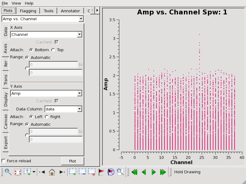
We flag the line emission using the flagdata task as follows:
# In CASA
flagdata(vis='TWHya_cont.ms', mode='manual', spw='1:24~24')
Next we will generate a first-pass continuum image. We will use mode "mfs" to generate a single continuum image from all the data.
# In CASA
os.system('rm -rf TWHya.continuum*')
clean(vis = 'TWHya_cont.ms',
  imagename = 'TWHya.continuum',
  field = '1', # TW Hya
  spw = '0~3',
  mode = 'mfs',
  imagermode = 'csclean',
  interactive=True,
  imsize = [300, 300],
  cell = '0.1arcsec',
  phasecenter = 1,
  weighting = 'briggs',
  robust = 0.5)
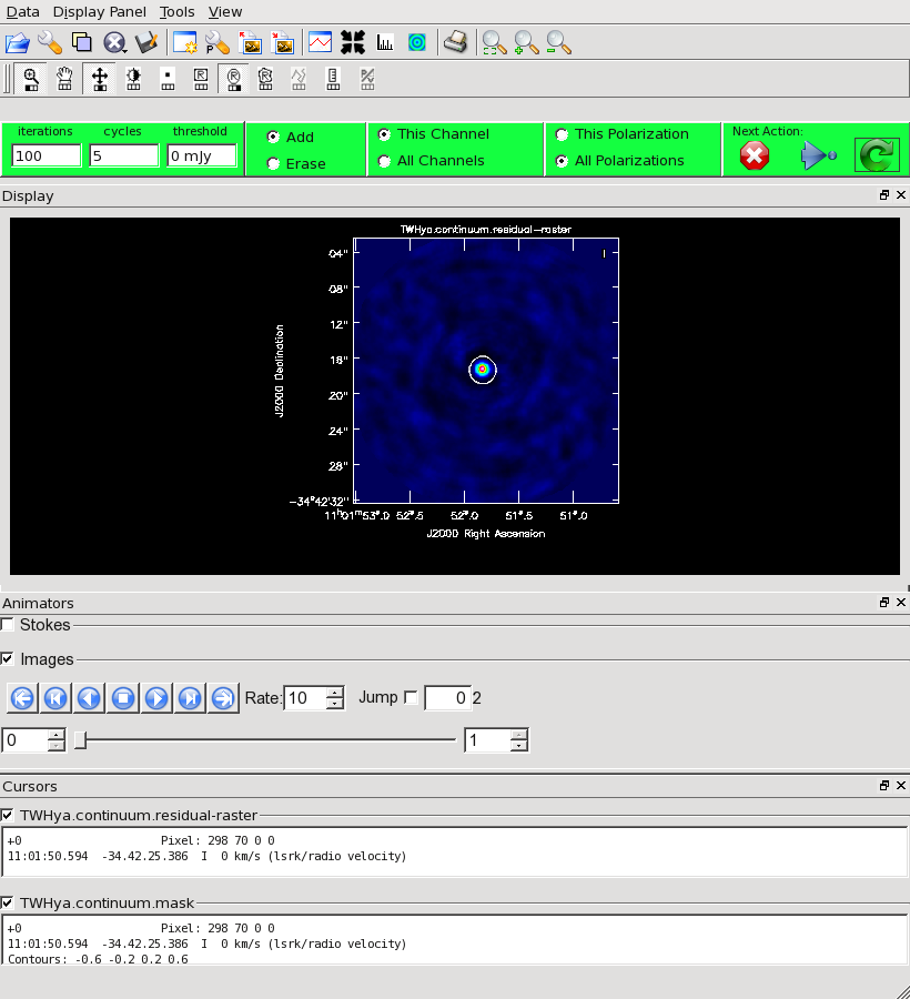
Note that at ~370 GHz the ALMA primary beam has a width of ~ 20 arcseconds FWHM. We want to image an area at least as large as that. Also, for this data set the synthesized beam is about 0.49 x 0.46 arcseconds. We have selected a cell size of 0.1 arcsec to fully sample the synthesized beam.
We'd like to do some cleaning to achieve our best image. In clean, the multifrequency synthesis mode grids each spectral channel independently. Since the uv-spacing is a function of frequency, this will actually achieve greater uv-coverage than if all the channels and spectral windows had been averaged in advance.
Our initial cleaned model will be used as the image model in the next self-calibration step. It is essential that only "real" signal be included in the image model, so we will clean the image conservatively. We set interactive=True to make the clean mask interactively. This also allows us to stop cleaning when the signal from the source starts to approach the surrounding "noise" areas in the residual map.
Once the Clean Viewer opens, click on the ellipse tool with your left mouse button, and draw a circle around the continuum emission with the left mouse button. Double click inside the region with the left mouse button when you are happy with it. It will turn from green to white when the clean mask is accepted. To begin the clean use the green arrow in the "Next action" section on the Viewer Display GUI.
The red X will stop clean, the blue arrow will clean non-interactively
until reaching the number of iterations requested (niter) or the flux
density threshold (whichever comes first), and the green circle arrow
will clean until it reaches the "iterations" parameter on the left side
of the green area.
You should choose the green circle arrow. It will clean 100 iterations (as shown in the GUI) and then show the residual image. If necessary you can adjust the color scale to examine the residuals more clearly. The middle mouse button is initially assigned to the "plus" icon, which adjusts the color scale. Also, note in the logger that clean reports the clean flux recovered so far, the min/max residuals, and the synthesized beam size.
In this example we will clean 500 iterations by clicking the green arrow five times, without changing the clean mask. After this we have cleaned about 1.5 Jy and we have residuals of about 5-7 mJy. Click the red and white "X" icon to conclude the cleaning process.
There are a few points to note:
- Real emission will not get cleaned if you do not put a clean box on it.
- Conversely, if you put a clean box on a region that contains no real emission and clean deeply, you can amplify any artifacts or features in that region.
- Thus, it's best to be conservative. Stop cleaning when the residuals inside the clean box approach those outside it. Start with a small clean box surrounding what is clearly real emission, and add to it after some iterations, if necessary. You can generally see fainter "real" features in the residuals.
- There is no default mask. So if you start an interactive clean and do not make a mask, the algorithm will clean nothing.
clean will generate several files:
- TWHya.continuum.flux # the effective primary beam response (e.g. for pbcor)
- TWHya.continuum.flux.pbcoverage # the primary beam coverage (ftmachine=’mosaic’ only)
- TWHya.continuum.image # the final restored image
- TWHya.continuum.mask # the clean mask
- TWHya.continuum.model # the model image
- TWHya.continuum.psf # the synthesized (dirty) beam
- TWHya.continuum.residual # the residual image
To examine the cleaned image with the CASA viewer, use:
# In CASA
viewer('TWHya.continuum.image')
First cycle of self-calibration: phase only
Next we can use the clean model to self-calibrate the uv-data. The process of self-calibration tries to adjust the data to better match the model you give it. That is why it is important to make the model as good as you can. clean places a uv-model of the resulting image in the file TWHydra_cont.model. This model can then be used to self-calibrate the data using gaincal. We use gaintype='T' to tell it to average the polarizations before deriving phase solutions (to improve sensitivity by a factor of sqrt(2)). The "solution interval" (solint) is critical and may require some experimentation to get optimal results. From listobs we see that the integration time of these data is 6.05 seconds, so we want to select a solution interval that is at least this long, and is matched to the expected coherence time of the atmosphere, while maintaining adequate S/N. We can use solint=30s as a starting point. It is often best to start with a larger solint and then work your way down to the integration time if the S/N of the data permits. For the reasons described in the TW Hydra Science Verification tutorial, we want to determine the phases before tackling amplitudes. Se we set calmode='p'.
# In CASA
gaincal(vis='TWHya_cont.ms',caltable='self_1.pcal',
        solint='30s',combine='',gaintype='T',
        refant='DV22',spw='',minblperant=4,
        calmode='p',minsnr=2)
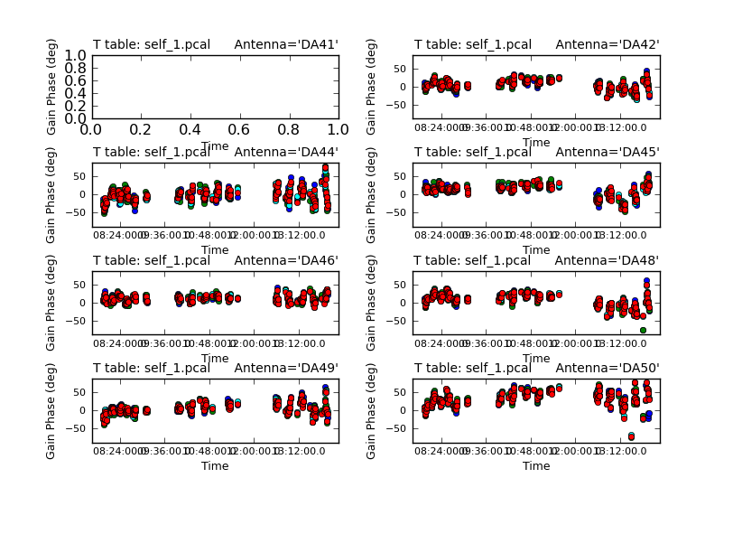
We are using combine=' ' to get independent solutions for each spw. If the S/N is insufficient to get independent solutions, you can try combining spectral windows with combine='spw'. We have plenty of S/N in these data so we keep them separate.
Next we'll examine the solutions using plotcal.
# In CASA
plotcal(caltable='self_1.pcal',xaxis='time',yaxis='phase',
        spw='',field='',iteration='antenna',
        subplot=421,plotrange=[0,0,-80,80],figfile='self_1_phase.png')
The magnitude of the corrections here gives you a sense of the accuracy of the phase transfer from the calibrators. Check that the phases are being well tracked by the solutions, i.e. smoothly varying functions of time within a given scan. Also the solutions for each spectral window should be nearly identical, indicating that the phase offsets between spectral windows are well calibrated already. In this example, the solutions look fine, overall. If they didn't you could try increasing the solint and/or combining the spw into a single solution.
When you are happy with the solutions, apply them with applycal
# In CASA
applycal(vis='TWHya_cont.ms',field='',gaintable=['self_1.pcal'],calwt=False)
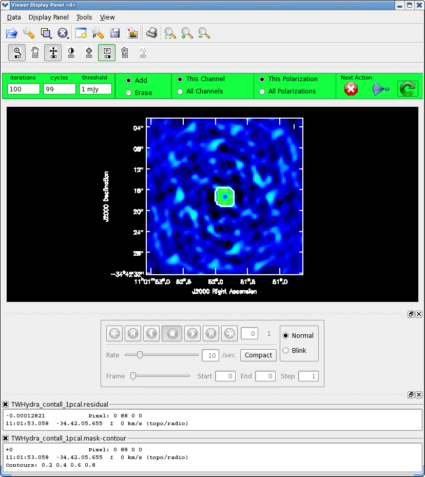
Next clean the source again. To save time we can start with the clean mask from the last iteration. If you make interactive adjustments to the clean mask, they will be written to the new mask TWHydra.continuum.1pcal.mask, and not the old one.
# In CASA
os.system('rm -rf TWHya.continuum.1pcal.*')
clean(vis='TWHya_cont.ms',imagename='TWHya.continuum.1pcal',
      mode='mfs',imagermode='csclean',
      imsize=300,cell=['0.1arcsec'],spw='',
      weighting='briggs',robust=0.5,
      mask='TWHya.continuum.mask',usescratch=False,
      interactive=True,threshold='1mJy',niter=10000)
Now after the first 500 iterations you see that the residuals inside the clean mask are higher than last time. This is because flux that had been spread out in the map due to poorly correlated phases has been recovered in the source, thereby increasing its flux. Let's continue cleaning for 1200 iterations.
Now let's compare the maps made before and after self-calibration using imview.
# In CASA
imview(raster=[{'file':'TWHya.continuum.image','range':[-0.01,0.05]},
       {'file':'TWHya.continuum.1pcal.image','range':[-0.01,0.05]}])
Once the Viewer Display panel opens, click on the box next in the "Images" panel and then use the tape deck buttons in the panel to alternate between the two images. We use the range parameter to put the two images on the same color scale. It is obvious that the self-calibrated image has much better residuals. To quantify the improvement in rms noise, use the rectangle tool to draw a region that excludes the central source and then double click inside. Repeat that process for the second image. Statistics for the region will print to the terminal:
(TWHya.continuum.image)
        Stokes       Velocity          Frame        Doppler      Frequency
             I   -10.5133km/s           LSRK          RADIO    3.65287e+11
BrightnessUnit       BeamArea           Npts            Sum    FluxDensity
       Jy/beam        25.4321          20100  -8.748308e-01  -3.439866e-02
          Mean            Rms        Std dev        Minimum        Maximum
 -4.352392e-05   2.133304e-03   2.132913e-03  -7.120122e-03   5.782832e-03
  region count
             1


(TWHya.continuum.1pcal.image)
        Stokes       Velocity          Frame        Doppler      Frequency
             I   -10.5133km/s           LSRK          RADIO    3.65287e+11
BrightnessUnit       BeamArea           Npts            Sum    FluxDensity
       Jy/beam        25.4701          20100  -4.660212e-02  -1.829681e-03
          Mean            Rms        Std dev        Minimum        Maximum
 -2.318513e-06   4.291876e-04   4.291920e-04  -1.593901e-03   1.666186e-03
  region count
             1
The self-calibrated image has improved the rms noise by a factor of 5.
Second cycle of self-calibration: phase only
Now that we have a better model, we can try to determine phase solutions again using a second round of phase-only self calibration. We will write the gain solutions to a new table, but these solutions will replace the solutions we determined in the first round. It may be useful to experiment with the solution interval. Keep in mind that the integration time is 6.05 seconds for this observation. (The integration time we refer to here is the "dump time" of the correlator, not the cumulative on-source time.)
In this example, we will stick with the 30 second solution interval.
# In CASA
os.system('rm -rf self_2*')
gaincal(vis='TWHya_cont.ms',caltable='self_2.pcal',
        solint='30s',combine='',gaintype='T',
        refant='DV22',spw='',minblperant=4,
        calmode='p',minsnr=2)
Now plot the new solutions.
# In CASA
plotcal(caltable='self_2.pcal',xaxis='time',yaxis='phase',
        spw='',field='',iteration='antenna',
        subplot=421,plotrange=[0,0,-80,80],figfile='self_2_phase.png')
The solutions look much the same as those after the first round of phase calibration, as expected, since the corrections from the (slightly better) new model are minor in this case. We can apply the new phase solutions and make a new image to see if there is improvement.
# In CASA
applycal(vis='TWHya_cont.ms',field='',gaintable=['self_2.pcal'],calwt=False)
Note, here, that applycal applies the gain solutions to the raw data and overwrites any results in the "corrected data" column of the measurement set, so this calibration replaces what we applied after the first-round solutions.
Now clean again, updating mask with the most recent mask file.
# In CASA
os.system('rm -rf TWHya.continuum.2pcal.*')
clean(vis='TWHya_cont.ms',imagename='TWHya.continuum.2pcal',
      mode='mfs',imagermode='csclean',
      imsize=300,cell=['0.1arcsec'],spw='',
      weighting='briggs',robust=0.5,usescratch=False,
      mask='TWHya.continuum.1pcal.mask',
      interactive=True,threshold='1mJy',niter=10000)
Clean again, interactively. In general, you should pay attention to the total flux being cleaned after each round, and the residuals inside the clean box as compared to those outside. When the cleaned flux in the latest round is small and the residuals inside the clean box match those outside it, the image has been sufficiently cleaned. Stop by hitting the red X on the GUI. In this case, let's again clean for 1200 iterations. The task reports a total cleaned flux and residuals similar to what we saw after the first round of cleaning:
Model 0: max, min residuals = 0.00105882, -0.00017499 clean flux 1.78282
Now repeat the display, blinking, and image statistics steps described above for the 1st and 2nd phase-only self-cal iterations.
# In CASA
imview(raster=[{'file':'TWHya.continuum.1pcal.image','range':[-0.01,0.05]},
       {'file':'TWHya.continuum.2pcal.image','range':[-0.01,0.05]}])
The second round made an improvement, but the difference is small:
(TWHya.continuum.1pcal.image)
        Stokes       Velocity          Frame        Doppler      Frequency
             I   -10.5133km/s           LSRK          RADIO    3.65287e+11
BrightnessUnit       BeamArea           Npts            Sum    FluxDensity
       Jy/beam        25.4696          21576  -7.237051e-02  -2.841450e-03
          Mean            Rms        Std dev        Minimum        Maximum
 -3.354213e-06   4.405892e-04   4.405866e-04  -1.534719e-03   1.791427e-03
  region count
             1
---- ---- ---- ---- ---- ---- ---- ---- ---- ---- ---- ---- ---- ---- ---- ---- ----
(TWHya.continuum.2pcal.image)
        Stokes       Velocity          Frame        Doppler      Frequency
             I   -10.5133km/s           LSRK          RADIO    3.65287e+11
BrightnessUnit       BeamArea           Npts            Sum    FluxDensity
       Jy/beam        25.3159          21576  -6.708313e-02  -2.649847e-03
          Mean            Rms        Std dev        Minimum        Maximum
 -3.109155e-06   4.225414e-04   4.225398e-04  -1.471975e-03   1.751540e-03
  region count
             1
This small improvement suggests that we have reached an end point with phase-only self-cal.
Third cycle of self-calibration: amplitude & phase
Next we will add amplitude self-calibration to the process. Amplitude changes more slowly than phase, so we will determine one solution per scan. We can set solint = 'inf', which tells gaincal to use the "combine" parameter to determine how to set the solution interval. With "combine" set to the default (combine = ) we will get one solution per scan.
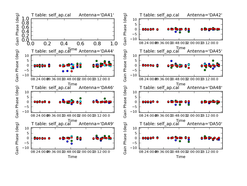
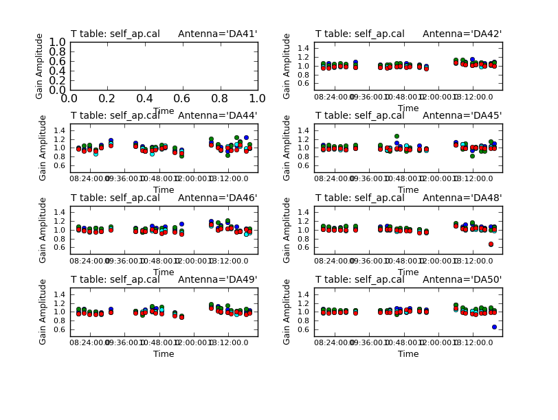
Also, note that we set "gaintable" to 'self_2.pcal'. This tells gaincal to apply the former phase-only solutions prior to determining the new amplitude+phase solutions. So, the new solutions will be incremental. Later when we apply these solutions to the data sets, we must be sure to apply both the phase-only solutions and the amplitude+phase solutions.
# In CASA
gaincal(vis='TWHya_cont.ms',caltable='self_ap.cal',
        solint='inf',combine='',gaintype='T',
        refant='DV22',spw='',minblperant=4,
        gaintable=['self_2.pcal'],
        calmode='ap',minsnr=2)

plotcal(caltable='self_ap.cal',xaxis='time',yaxis='phase',
        spw='',field='',antenna='',iteration='antenna',
        subplot=421,plotrange=[0,0,-10,10],figfile='self_ap_phase.png')

plotcal(caltable='self_ap.cal',xaxis='time',yaxis='amp',
        spw='',field='',antenna='',iteration='antenna',
        subplot=421,plotrange=[0,0,0.5,1.5],figfile='self_ap_amp.png')
Use the "next" button on the plotcal GUI to advance the plot to see additional antennas. Since phase corrections have already been applied, we see that the new incremental phase solutions are fairly small. The amplitude corrections are at the level of ~10% in many cases, but there is considerable variance among different antennas. See Figures 6 and 7 for the phase and amplitude solutions.
We can apply the calibration now with applycal. Note we apply two gain tables.
# In CASA
applycal(vis='TWHya_cont.ms',field='',gaintable=['self_2.pcal','self_ap.cal'],calwt=False)
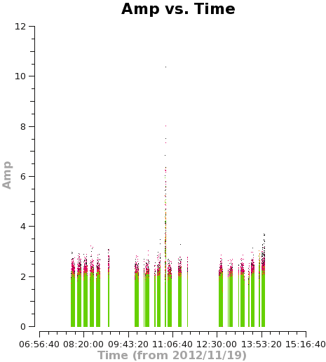
Let's plot the u,v data against both time and u,v distance. It is a good idea to check these after an amplitude self-calbration to be sure that it worked properly. Occasionally, a few spurious bits of data will get wildly incorrect values by the amplitude self-cal.
# In CASA
plotms(vis='TWHya_cont.ms',xaxis='time',yaxis='amp',
       avgchannel='38',ydatacolumn='corrected',coloraxis='spw',
       plotfile='selfcal_time.png')

# In CASA
plotms(vis='TWHya_cont.ms',xaxis='uvdist',yaxis='amp',
       avgchannel='38',ydatacolumn='corrected',coloraxis='spw',
       plotfile='selfcal_uvdist.png')
Figures 8 and 9 show results from the previous two commands.
Using the "locate" tool in the plotms GUI, select a few bad data points and confirm the scan number. We can see that bad data points exist for, at least, spw 0 and 1. To be conservative, we can flag all of scan 72. It's not much data compared to the full observation.
# In CASA
flagdata(vis='TWHya_cont.ms', mode='manual', scan='72')
Replot the u,v data to confirm the bad data have been removed. IMPORTANT: when re-plotting this data set in plotms, you must remember to select the "force reload" button on the GUI. Otherwise, the plot will not update with the new flags.
If the plots look good, you can proceed to make the final continuum image.
# In CASA
os.system('rm -rf TWHya.continuum.apcal.*')
clean(vis='TWHya_cont.ms',imagename='TWHya.continuum.apcal',
      mode='mfs',imagermode='csclean',
      imsize=300,cell=['0.1arcsec'],spw='',
      weighting='briggs',robust=0.5,usescratch=False,
      interactive=True,threshold='0.1mJy',niter=5000,npercycle=1000)
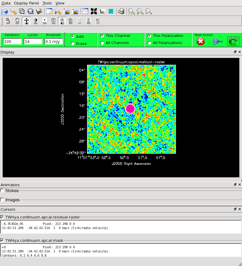
You will need to execute over a thousand iterations in total to get the image fully cleaned, so we start the clean process with 1000 iterations and press the green circle. In the GUI, you should then adjust the number of iterations per cycle down to 100 for additional cleaning. Update the clean box if necessary, by expanding the region with a larger ellipse. Note that the pattern of residuals inside the clean box may not come to match that outside it, but you want to clean until the magnitude of the residuals is similar, inside it and out. In this case, the cleaning takes about 1500 iterations.
The clean task reports a total cleaned flux of 1.76 Jy.
# In CASA
imview(raster=[{'file':'TWHya.continuum.2pcal.image','range':[-0.01,0.05]},
       {'file':'TWHya.continuum.apcal.image','range':[-0.01,0.05]}])
(TWHya.continuum.2pcal.image)
        Stokes       Velocity          Frame        Doppler      Frequency
             I   -10.5133km/s           LSRK          RADIO    3.65287e+11
BrightnessUnit       BeamArea           Npts            Sum    FluxDensity
       Jy/beam        25.3159          20553   1.654666e-01   6.536086e-03
          Mean            Rms        Std dev        Minimum        Maximum
  8.050727e-06   4.115417e-04   4.114729e-04  -1.471975e-03   1.612787e-03
  region count
             1
---- ---- ---- ---- ---- ---- ---- ---- ---- ---- ---- ---- ---- ---- ---- ---- ----
(TWHya.continuum.apcal.image)
        Stokes       Velocity          Frame        Doppler      Frequency
             I   -10.5133km/s           LSRK          RADIO    3.65287e+11
BrightnessUnit       BeamArea           Npts            Sum    FluxDensity
       Jy/beam        25.3653          20553   3.826559e-02   1.508581e-03
          Mean            Rms        Std dev        Minimum        Maximum
  1.861801e-06   2.410208e-04   2.410195e-04  -1.023332e-03   8.470871e-04
  region count
             1
We see that the amplitude+phase self-cal made a significant improvement in the rms of the image, compared to the phase-only self-cal from 0.41 mJy to 0.24 mJy.
Apply Calibration to the Full Data Set and Split the Line Data
Now we apply the self-calibration derived from the continuum emission to the full-resolution spectral cube.
# In CASA
applycal(vis='calibrated.ms',gaintable=['self_2.pcal','self_ap.cal'],calwt=False)
Remember to flag the bad scan, 72.
# In CASA
flagdata(vis='calibrated.ms',scan='72')
Next we can split off the spectral line data for further processing.
# In CASA
os.system('rm -rf TWHydra_H2D+.ms*')
split(vis='calibrated.ms',outputvis='TWHydra_H2D+.ms',datacolumn='corrected',spw='0',field='TW Hya')

os.system('rm -rf TWHydra_N2H+.ms*')
split(vis='calibrated.ms',outputvis='TWHydra_N2H+.ms',datacolumn='corrected',spw='1',field='TW Hya')
Subtracting the Continuum
The next step in the processing is to subtract the continuum from the full data set, in preparation for imaging the line emission. We'll do the subtraction in the u,v plane. We determine the continuum from line-free channels, so we begin by plotting the u,v amplitudes using plotms, to identify channels with the N2H+ line.
# In CASA
plotms(vis='TWHydra_N2H+.ms',xaxis='channel',yaxis='amp',avgtime='1e8',avgscan=True)
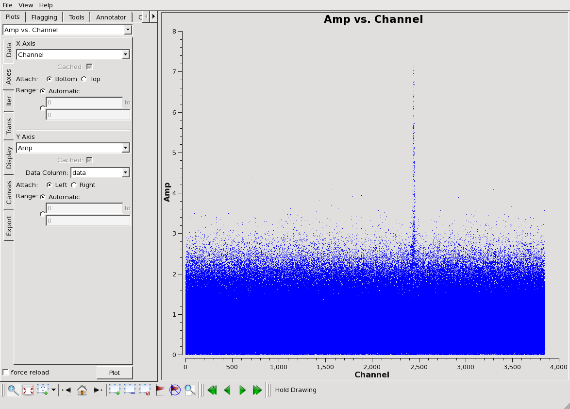
In this data set, the line emission is evident directly in the u,v amplitudes. Although the line is not really strong enough to have much impact on continuum subtraction, we will avoid the N2H+ line anyway (good practice) and fit the continuum to the spectrum using line-free channels. In fitting for the continuum we will also avoid a few channels at the band edges, where there can sometimes be erratic data.
# In CASA
uvcontsub(vis='TWHydra_N2H+.ms',fitorder=1,fitspw='0:20~2400,0:2500~3800')
It is useful at this stage to determine the velocity range of the detected emission. We'll use this later when we image the line emission. Using the plotms GUI, set the X axis to "Velocity" and then select the vertical "Trans" tab. Here, set the Frame to "LSRK", the velocity defn to "RADIO", and the Rest Freq to 372672.49 MHz. Then re-plot the data by clicking the "Plot" button. Notice that the emission falls between ~ 2-4 km/s, which is consistent with the known recession velocity of TW Hydra, about 2.9 km/s.
Imaging N2H+
The final step is to image the N2H+ line emission using the {clean}} task.
Many of the imaging parameters are the same as we used for the continuum, but now we have a few new parameters to set for the spectral cube: mode, start, width, nchan, restfreq, and outframe. When making spectral images you have three choices for mode: "channel", "velocity", or "frequency". The data are recorded into channels spaced by a constant frequency increment, but for spectral line analysis it's often more useful to have a constant velocity increment. For mode='velocity', the desired start and width also need to be given in velocity units.
ALMA does not do on-line Doppler Tracking and the native frame of the data is topocentric (TOPO). If you do not specify outframe, the output cube will also be in TOPO, which is not very useful for spectral line work. By specifying the outframe parameter, clean will make the doppler shift correction. Alternatively it can be done prior to imaging with the cvel task.
In our example here, we will image the N2H+ line in the range 0-4 km/s using steps of 0.1 km/s. Our choice of velocity increment is determined by the channel spacing. From the listobs output, we know the channel spacing is 61 kHz, which corresponds to ~ 0.05 km/s at 372 GHz. The true velocity resolution is worse than the channel spacing by about a factor of 2. So, 0.1 km/s steps in velocity is a good choice.
# In CASA
os.system('rm -rf line.N2H+.*')
clean(vis = 'TWHydra_N2H+.ms.contsub', imagename = 'line.N2H+', mode = 'velocity', nchan = 40, start = '1.0km/s',
  width = '0.1km/s', outframe = 'LSRK', restfreq = '372.67249GHz', imagermode = 'csclean',
  interactive=True, niter=1000, imsize = [300, 300], cell = '0.1arcsec', weighting = 'briggs', robust = 0.0)
Imaging spectral data cubes with complex line emission can be an arduous task. In this case, we use the clean viewer to step through each spectral channel and define a clean mask for each channel individually. This is usually the best approach when the structure is complex and changing from one spectral channel to the next, as it is for the N2H+ line in TW Hydra. For simpler structures, it can be sufficient to define a single clean mask and apply it for all channels.
After the viewer GUI appears, you may wish to maximize the size of the "Display" panel by deselecting the "Cursors" panel, if necessary. Then step through channels with the tape deck controls, and create a clean mask for each channel with detected line emission, as you did for the continuum cleaning. In this case, make sure that the radio button at the top of the GUI has "This Channel" selected, to create a separate mask for each spectral channel.
Click the green arrow to clean with 100 iterations, then click the "play" button on the tape deck to see the residuals, You will see significant residuals remaining in each channel. Continue cleaning until the residuals inside the clean boxes match those outside. If you reach 5000 iterations, the clean task will end itself (since we specified niter=5000). If you'd like to stop sooner, click the red "X" button.
That's it! You've got a data cube with N2H+ ready for analysis.
Apart from imaging this targeted channel range, it is also important to image the full data cube to explore the full spectral bandwidth observed. A full imaging could be accomplished as follows:
# In CASA
os.system('rm -rf line.N2H+.*')
clean(vis = 'TWHydra_N2H+.ms.contsub', imagename = 'line.N2H+', mode = 'channel', start=0, width=10, imagermode = 'csclean',
  interactive=False, niter=0, imsize = [300, 300], cell = '0.1arcsec', weighting = 'briggs', robust = 0.0)
What About the H2D+?
Recall the first spectral window (spw='0') in the calibrated.ms data set contains the anticipated H2D+ line emission. Imaging of that line can proceed in much the same manner as we have done for the N2D+ line. In this case, though, there is no obvious detection of the H2D+ line. So we will not repeat the steps in this guide.
Image Analysis
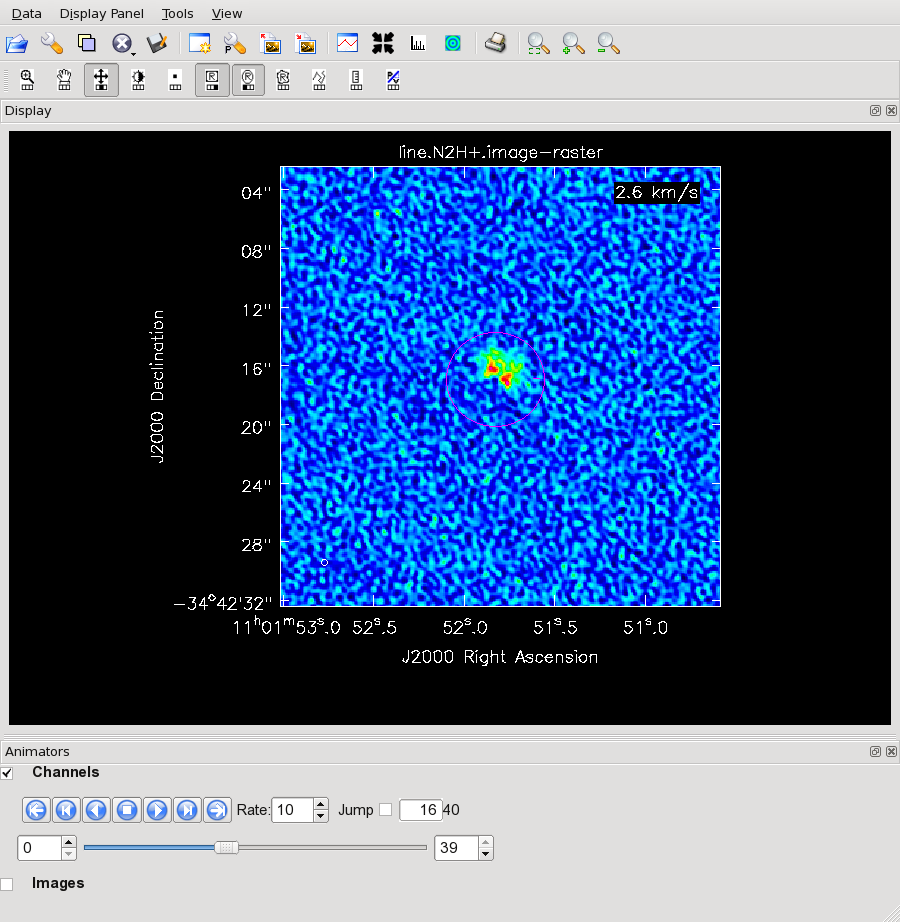
The CASA viewer offers some powerful capabilities for exploring spectral data cubes. We are currently preparing CASA Guides that discuss Using the Viewer to Extract Spectra, and Making Moment Maps. Check back later!
Here, we will demonstrate how to make moment maps from the N2H+ data cube. First examine the final image in the viewer:
# In CASA
viewer('line.N2H+.image')
You should see a result as shown in Figure 12.
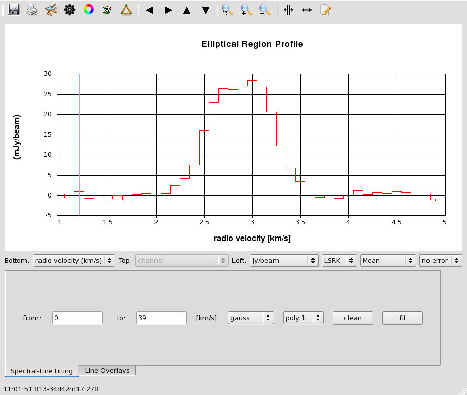
Use the ellipse drawing tool to define an elliptical region that encompasses all the line emission, from all channels, and then select "Spectral Profile" from the "Tools" menu to generate a spectrum, as shown in Figure 13 to the right. We are showing the X axis in units of velocity. If we select "channels" from the Spectral Profile GUI, we can see that the line emission extends from channels 11-26.
Now make the Moment 0 map:
# In CASA
os.system('rm -rf line.N2H+.image.mom0')
immoments(imagename='line.N2H+.image',moments=[0], outfile='line.N2H+.image.mom0', chans='11~26')
# In CASA
os.system('rm -rf ')
os.system('rm -rf ')
immoments(imagename='line.N2H+.image',moments=[1,2],
          outfile='line.N2H+.image.mom',
          chans='11~26',includepix=[0.1,100])
Display all three moment maps in the viewer, overlaid with continuum contours.
# In CASA
imview( raster=[ {'file':'line.N2H+.image.mom0'},
                 {'file':'line.N2H+.image.mom.weighted_coord'},
                 {'file':'line.N2H+.image.mom.weighted_dispersion_coord'} ],
        contour={'file':'TWHya.continuum.apcal.image', 'base':0, 'unit':0.0025, 'levels':[3,100]} )
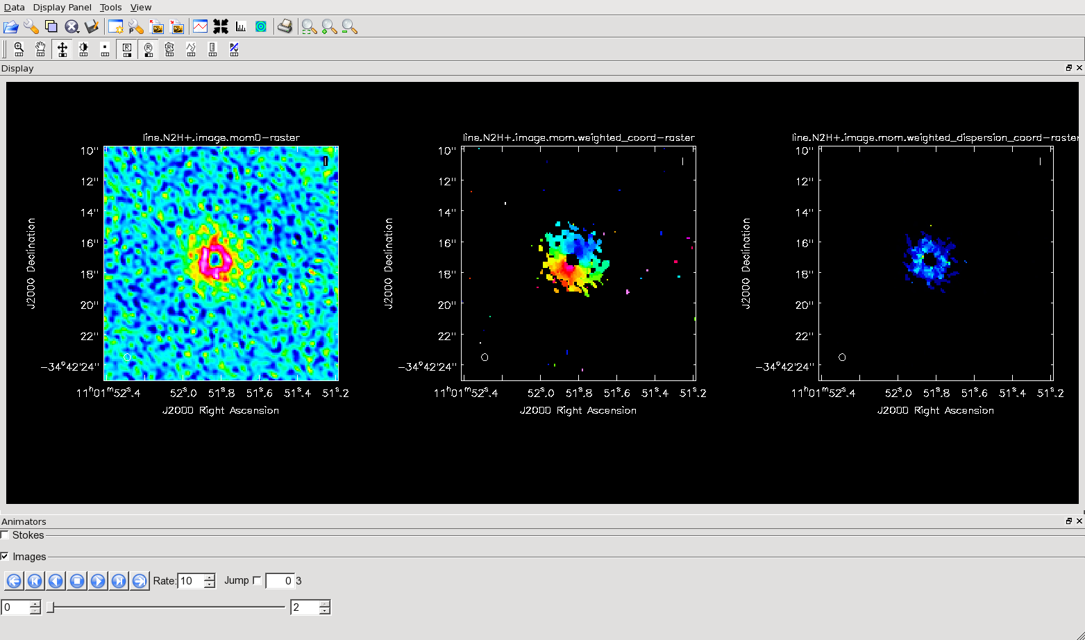
To see all three raster images simultaneously, open the viewer's Panel Display Options (the "P-wrench" icon in the viewer tool bar), click "Number of panels", and change "Number of panels in x" to 3.