ACA Simulation (CASA 4.0): Difference between revisions
| (One intermediate revision by the same user not shown) | |||
| Line 143: | Line 143: | ||
Next we use '''simanalyze''' to combine the three measurement sets and create a single image. | Next we use '''simanalyze''' to combine the three measurement sets and create a single image. | ||
There are many ways to do this, and | There are many ways to do this, and you may wish to discuss options with scientists at your ARC. In this example we will use the total power image as a model when deconvolving the ACA image, and then use the result as a model when deconvolving the 12m interferometric image. This method tends to give low weight to the large spatial scales, but is simple to illustrate. | ||
It's possible to get better results if one used multiscale clean in the clean task (again using the lower resolution image as a model when deconvolving the higher resolution one). An alternative would be to create an image independently from each dataset, and then use the CASA feather task to combine them entirely in the image plane. | |||
If given a total power and interferometric measurement set, '''simanalyze''' will automatically create the total power image, | |||
then use it as a model and deconvolve the interferometric image. It is not recommended to do both interferometric images simultaneously. | then use it as a model and deconvolve the interferometric image. It is not recommended to do both interferometric images simultaneously. | ||
| Line 170: | Line 168: | ||
====Next add the 12m interferometric data==== | ====Next add the 12m interferometric data==== | ||
[[Image:M51c.ALMA_0.5arcsec.analysis.3.4.png|thumb|TP+ACA combined (with relatively low weight) with 12m ALMA]] | [[Image:M51c.ALMA_0.5arcsec.analysis.3.4.png|thumb|TP+ACA combined (with relatively low weight) with 12m ALMA]] | ||
Here we explicitly have to set the modelimage to the previous | Here we explicitly have to set the ''modelimage'' to the result from the previous run. | ||
<source lang="python"> | <source lang="python"> | ||
Latest revision as of 22:45, 28 November 2012
↵ Simulating Observations in CASA
To create a script of the Python code on this page see Extracting scripts from these tutorials.
ALMA 12m + ACA + Total Power
We can simulate ALMA observations that use the main array of 12 m antennas augmented by the ACA and Total Power antennas by generating simulated observations for each component separately, and then combining the Measurement Sets in simanalyze. This technique is general and can be used to simulate observations using multiple 12 m array configurations, as well. Total power observations can be simulated either in an independent run of simobserve, or along with an interferometric simulation. Note that if you simulate total power and an interferometric observation simultaneously with simobserve, they must have the same set of pointing centers and the same integration and total time, which is probably not realistic. (For example it is generally recommended to observe a larger area by 1/2 primary beam in total power mode to combine with a 12 m ALMA mosaic).
Set simobserve as current task
Reset all parameters to default, and then set the project name to m51c
# Set simobserve to default parameters
default("simobserve")
# Our project name will be m51c, and all simulation products will be placed in a subdirectory m51c/
project="m51c"
Specify sky model image
We'll use an Halpha image of M51 as a model of the sky, for this example. The curl command will copy the file from a URL and rename it.
# Model sky = Halpha image of M51
os.system('curl http://casaguides.nrao.edu/images/3/3f/M51ha.fits.txt -f -o M51ha.fits')
skymodel         =  "M51ha.fits"
Note that simobserve will not modify your original input image. Rather, it will make a copy m51c/m51c.skymodel.
We will override most of the parameters in the Halpha FITS image to make the image more suitable to a sub-millimeter ALMA observation. We will:
- place the source in the southern hemisphere with the indirection parameter,
- set the pixel size to 0.1arcsec, to simulate an observation of a galaxy that is smaller in angular size. (M51 itself would require a quite large mosaic, and in any case we'd like the input model pixels to be significantly smaller than the synthesized beam.)
- set the peak brightness to 0.004 Jy/pixel
- set the frequency to 330GHz, and since it's a 2D image we'll set the single "channel" width to be 50MHz, and peak brightness of 0.004 Jy/pixel. These parameters are plausible for observing a sub-mm emission line in a galaxy.
# Set model image parameters:
indirection="B1950 23h59m59.96s -34d59m59.50s"
incell="0.1arcsec"
inbright="0.004"
incenter="330.076GHz"
inwidth="50MHz"
Simulate 12m interferometric observation
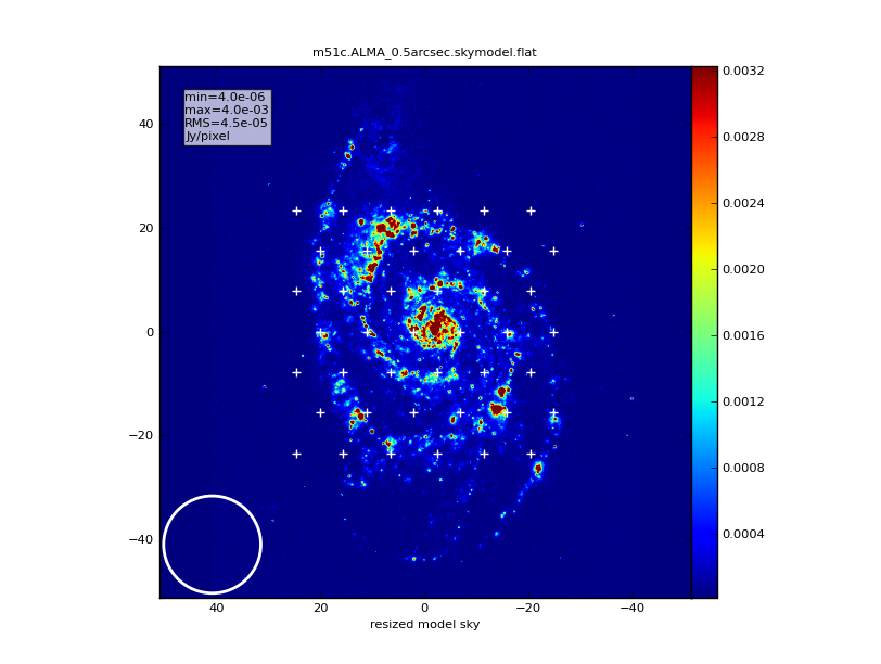
We'll begin by simulating the observation as seen by the main 12 m ALMA array. We'll have simobserve calculate a hexagonal mosaic of pointings.
The interface for simobserve provides an integration parameter, which is the dwell time at each pointing in the mosaic. We'll set that to 10 s. A real observation might dwell on each pointing for ~ 20 s and record 3 sets of visibilities (i.e. 6 s integration time) for each pointing. simobserve does not currently offer a capability to reproduce this behavior exactly, but the difference in UV coverage should be very minor between the real observation and the simulated one. You could try setting integration to ~ 20 s, which would more closely match the dwell time for some real observations.
# have simobserve calculate mosaic pointing locations:
setpointings       =  True
integration        =  "10s"
mapsize            =  "1arcmin"
maptype            =  "hex"
pointingspacing    =  "9arcsec"      # this could also be specified in units of the primary beam e.g. "0.5PB"
Calculate Visibilities
When you provide a desired resolution in the antennalist parameter, simobserve will determine what array configuration to use.
obsmode            =  "int"
antennalist        =  "ALMA;0.5arcsec"
totaltime          =  "3600s"
Run simobserve, displaying graphics to the screen and also writing graphics output to files that can be found in the project directory, m51c.
graphics           =  "both"
simobserve()
Simulate 12m total power observation
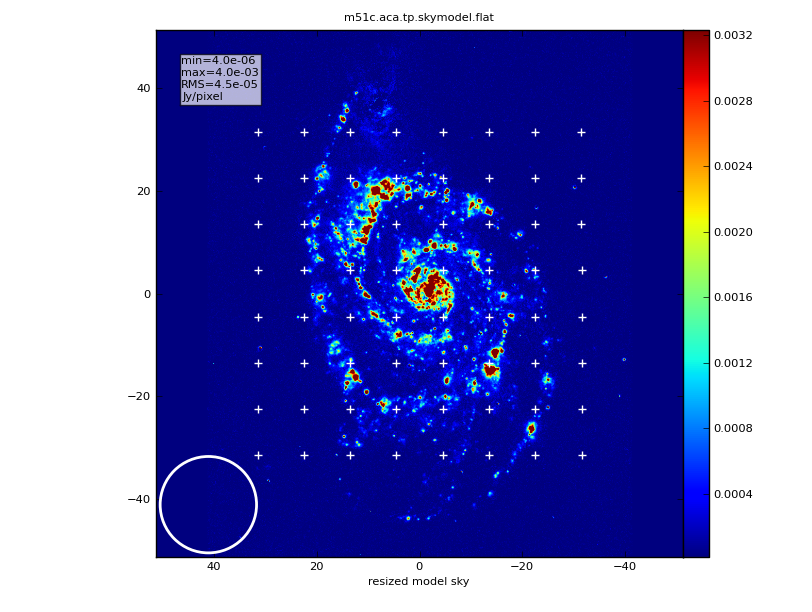
Next we'll simulate a total power raster map of the same area, on a square grid. CASA simulation tools can not simulate true on-the-fly mapping (with smearing on timescales smaller than an integration time), but a square grid with a short integration time will provide a very accurate approximation.
By virtue of CASA's global parameters, we already have project and image world coordinate system parameters set correctly.
We need to change the mapping parameters to specify a square region a bit larger than the interferometric map.
integration        =  "10s"
mapsize            =  "1.3arcmin"
maptype            =  "square"
We'll observe on a different day. This doesn't really matter, but if you choose to simulate two different 12m ALMA configurations and combine them, you will have issues concatenating the datasets if they are simulated on the same day with the same antenna names. So, it's a good habit to change the day.
obsmode            = "sd"
sdantlist          = "aca.tp.cfg"
sdant              = 0
refdate            = "2012/12/01"
totaltime          =  "2h"
Run simobserve, displaying graphics to screen and to files.
simobserve()
Simulate 7m ACA observation
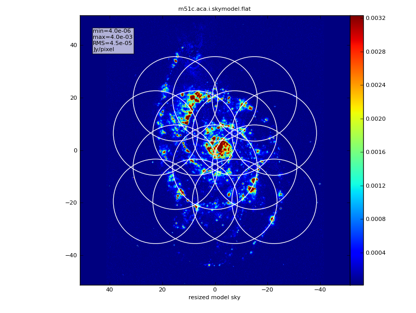
Next we'll add an ACA mosaic, with its larger primary beam.
integration        =  "10s"
mapsize            =  "1arcmin"
maptype            =  "hex"
pointingspacing    =  "15arcsec"
We can specify an integral number of times to repeat the mosaic by setting totaltime to an integer string without units.
obsmode            = "int"
refdate            = "2012/12/02"
antennalist        =  "aca.i.cfg"
totaltime          =  "3"
Run simobserve, displaying graphics to screen and to files.
simobserve()
Deconvolve the visibilities back into an image
Next we use simanalyze to combine the three measurement sets and create a single image.
There are many ways to do this, and you may wish to discuss options with scientists at your ARC. In this example we will use the total power image as a model when deconvolving the ACA image, and then use the result as a model when deconvolving the 12m interferometric image. This method tends to give low weight to the large spatial scales, but is simple to illustrate.
It's possible to get better results if one used multiscale clean in the clean task (again using the lower resolution image as a model when deconvolving the higher resolution one). An alternative would be to create an image independently from each dataset, and then use the CASA feather task to combine them entirely in the image plane.
If given a total power and interferometric measurement set, simanalyze will automatically create the total power image, then use it as a model and deconvolve the interferometric image. It is not recommended to do both interferometric images simultaneously.
First image total power and ACA with total power as a model
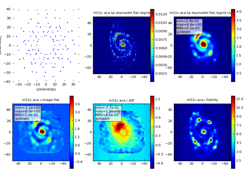
default("simanalyze")
project            =  "m51c"
vis                =  '$project.aca.i.ms,$project.aca.tp.sd.ms'
imsize             =  [512,512]
cell               =  '0.2arcsec'
analyze            =  True
showpsf            =  False
showresidual       =  False
showconvolved      =  True
simanalyze()
Next add the 12m interferometric data
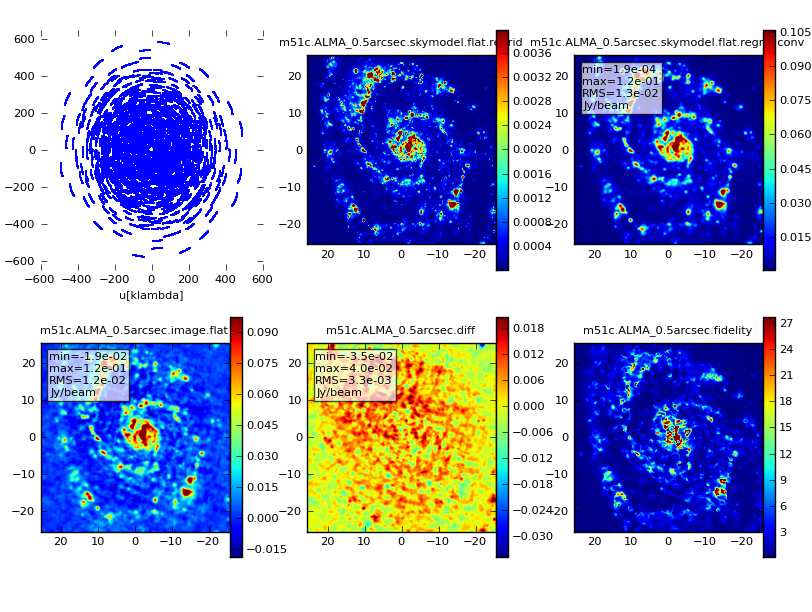
Here we explicitly have to set the modelimage to the result from the previous run.
default("simanalyze")
project            =  "m51c"
vis                =  '$project.ALMA_0.5arcsec.ms'
imsize             =  [512,512]
cell               =  '0.1arcsec'
modelimage         =  "$project.aca.i.image"
analyze            =  True
showpsf            =  False
showresidual       =  False
showconvolved      =  True
simanalyze()
↵ Simulating Observations in CASA
Last checked on CASA Version 4.0.0.