Predict: Difference between revisions
No edit summary |
|||
| (3 intermediate revisions by one other user not shown) | |||
| Line 1: | Line 1: | ||
{{Simulations Intro}} | {{Simulations Intro 4.0}} | ||
[[Category: Simulations]] | [[Category: Simulations]] | ||
| Line 5: | Line 5: | ||
Once you have a sky model with appropriate Coordinate System and a list of pointings, you can calculate visibilities. simobserve can additionally predict from a Component List named '''complist''' (see below). | Once you have a sky model with appropriate Coordinate System and a list of pointings, you can calculate visibilities. simobserve can additionally predict from a Component List named '''complist''' (see below). | ||
We only discuss interferometric visibilities here but the process is similar for single dish simulated observations ('''obsmode''' = "sd") -- see the [[ACA Simulation (CASA 3.4) | We only discuss interferometric visibilities here but the process is similar for single dish simulated observations ('''obsmode''' = "sd") -- see the [[ACA Simulation (CASA 3.4)|ACA Guide]]. | ||
| Line 33: | Line 33: | ||
here is a little python program [[File:makecl_py.txt]] that will change this ascii file [[File:my_list.txt]] into a componentlist | here is a little python program [[File:makecl_py.txt]] that will change this ascii file [[File:my_list.txt]] into a componentlist | ||
a more complete guide to componentlist simulation is [[Comp list guide]] | a more complete guide to componentlist simulation is [[Simulation Guide Component Lists (CASA 3.4)|Comp list guide]] | ||
== Graphic Output == | == Graphic Output == | ||
Latest revision as of 15:17, 2 November 2012
↵ Simulating Observations in CASA
Calculating Visibilities (obsmode = "int")
Once you have a sky model with appropriate Coordinate System and a list of pointings, you can calculate visibilities. simobserve can additionally predict from a Component List named complist (see below). We only discuss interferometric visibilities here but the process is similar for single dish simulated observations (obsmode = "sd") -- see the ACA Guide.
- antennalist is a text file containing the antenna locations (see Antenna List for details)
- refdate, hourangle, and totaltime set when you want to observe and for how long.
- More flexibility of hour angle, e.g. for snapshot observations through a range of LST, are currently best achieved by simulating a long track, flagging the timerange near zenith with flagdata, leaving an off-zenith unflagged time range, and then running clean on the ms, either with the clean task, or with simanalyze.
- Mosaic observations will rotate through the mosaic fields during the track defined by totaltime, remaining at each pointing for a duration integration. No slew time is inserted. totaltime can be an integer without units, in which case it will cycle through the mosaic that many times.
- One can interleave a calibrator in direction caldirection and flux calflux with one's science pointings. The pointing file should contain the science mosaic, not the calibrator. simobserve will observe all pointings of the pointing file, then the calibrator for the same integration time, then the pointings in the pointing file again, etc, until totaltime is used up.
- If obsmode = "sd" is set, simobserve will create $project.sd.ms, otherwise it will create $project_$configuration.ms.
Component list
One way to get a component list is to deconvolve an image, and another is to create it by hand using the cl tool:
cl.done()
cl.addcomponent(dir="J2000 18h00m00.03s -42d0m0.0s", flux=1.0, freq='672.0GHz')
cl.rename("star672GHz.cl")
complist = "star672GHz.cl"
here is a little python program File:Makecl py.txt that will change this ascii file File:My list.txt into a componentlist
a more complete guide to componentlist simulation is Comp list guide
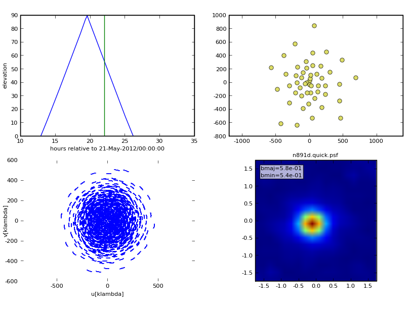
Graphic Output
If you have graphics turned on, you'll see a diagnostic plot like this one:
