TWHydraBand7 SS12 Overview: Difference between revisions
No edit summary |
|||
| (10 intermediate revisions by the same user not shown) | |||
| Line 1: | Line 1: | ||
* '''Calibration portion of the tutorial:''' [[TWHydraBand7_SS12]] | |||
* '''Imaging portion of the tutorial:''' [[TwHydraBand7_Imaging_SS12]] | |||
[[Category:ALMA]][[Category:Calibration]][[Category:Spectral Line]] | [[Category:ALMA]][[Category:Calibration]][[Category:Spectral Line]] | ||
| Line 20: | Line 21: | ||
[[Image:Qi_HCOp3_2.gif|thumb|SMA HCO+(3-2) emission from TW Hya (Qi et al. 2008; Figure 2).]] | [[Image:Qi_HCOp3_2.gif|thumb|SMA HCO+(3-2) emission from TW Hya (Qi et al. 2008; Figure 2).]] | ||
ALMA Science Verification data at Band 7 (~345 GHz) was taken for TW Hya on April 22, 2011. A scheduling block about 1.5 hours long was run three times in a row for a total of about 4.5 hours of observing time. The names of the three ASDMs were: uid://A002/X1d9d21/X3c1, uid://A002/X1d9d21/X5d8 and uid://A002/X1d9d21/X7df. | ALMA Science Verification data at Band 7 (~345 GHz) was taken for TW Hya on April 22, 2011. A scheduling block about 1.5 hours long was run three times in a row for a total of about 4.5 hours of observing time. The names of the three data sets ('ALMA Science Data Models' - ASDMs) were: uid://A002/X1d9d21/X3c1, uid://A002/X1d9d21/X5d8, and uid://A002/X1d9d21/X7df. | ||
<pre style="background-color: #ffa07a;"> | |||
In order to ensure that you can work through the whole reduction in one morning, we focus the | |||
calibration guide on the first data set, "X3c1" for short. We provide all three data sets for | |||
imaging. | |||
</pre> | |||
Nine antennas were available during these runs, but one has to be flagged. All four available basebands were used, resulting in four spectral windows (spws) containing data. Two basebands were placed in the Lower Sideband (LSB) and two basebands in the Upper Sideband (USB). In the LSB the CO(3-2) line at a rest frequency of 345.79599 GHz is located in spw=2. In the USB the HCO+(4-3) line at a rest frequency of 356.7342 GHz is located in spw=0. The other two spectral windows do not contain strong spectral lines and are used for continuum. Each spectral window is 0.5 GHz wide and the channel width is 122 kHz. Because the ALMA correlator was configured to apply Hanning smoothing of the signal, the effective spectral resolution is about twice the channel width, which in this case is about 0.2 km/s. For the antenna configuration in use at the time, the angular resolution is expected to be about 1.5". The median value of precipitable water vapor (PWV) for this period was 1.16 mm, as measured by the water vapor radiometers. This PWV corresponds to an opacity of 0.20 at the CO(3-2) line. The mean wind speed was 6.2 m/s. | Nine antennas were available during these runs, but one has to be flagged. All four available basebands were used, resulting in four spectral windows (spws) containing data. Two basebands were placed in the Lower Sideband (LSB) and two basebands in the Upper Sideband (USB). In the LSB the CO(3-2) line at a rest frequency of 345.79599 GHz is located in spw=2. In the USB the HCO+(4-3) line at a rest frequency of 356.7342 GHz is located in spw=0. The other two spectral windows do not contain strong spectral lines and are used for continuum. Each spectral window is 0.5 GHz wide and the channel width is 122 kHz. Because the ALMA correlator was configured to apply Hanning smoothing of the signal, the effective spectral resolution is about twice the channel width, which in this case is about 0.2 km/s. For the antenna configuration in use at the time, the angular resolution is expected to be about 1.5". The median value of precipitable water vapor (PWV) for this period was 1.16 mm, as measured by the water vapor radiometers. This PWV corresponds to an opacity of 0.20 at the CO(3-2) line. The mean wind speed was 6.2 m/s. | ||
| Line 34: | Line 39: | ||
==Obtaining the Data== | ==Obtaining the Data== | ||
We have provided the data for you on the tutorial computers. The calibration and imaging portions of the guide will step you through how to get started. | |||
Once you return to your home institution, you may want to follow the full version of the CASA guide. In this case the data are available via the ALMA science portal [http://almascience.nrao.edu/almadata/sciver/TWHya here] . | |||
==TWHya Data Reduction Tutorial== | ==TWHya Data Reduction Tutorial== | ||
The tutorial has two main parts. We will spend the morning on calibration of the data and then the afternoon imaging the calibrated data (and using these images to further refine the calibration). There is a separate page for each part of the tutorial: | |||
''' | # '''[[TWHydraBand7_SS12]]''' this page steps you through the morning calibration tutorial. | ||
# '''[[TwHydraBand7_Imaging_SS12]]''' this page steps you through the afternoon imaging and self-calibration tutorial. | |||
''' | |||
==How to Use A CASA guide== | |||
In the guides | In the guides | ||
| Line 86: | Line 70: | ||
This color shows you background information about the data or other types of reference material | This color shows you background information about the data or other types of reference material | ||
</pre> | </pre> | ||
<pre style="background-color: #ffa07a;"> | |||
This color shows summer-school-specific notes. | |||
</pre> | |||
A few tips on using CASA (copied from the EVLA IRC+10216 tutorial): | |||
[[Image:clean.png|thumb|Inputs from one of the clean commands from this tutorial]] | |||
There are a number of possible ways to run CASA. Many aspects are described in [[Getting_Started_in_CASA]]. You should review this page if you are new to CASA. In brief you can run CASA interactively by looking at the inputs to tasks with '''inp taskname''' (example: inp clean), setting the parameters one by one (example: selectdata=T) as you desire and then run '''go'''. After setting parameters one by one in a task and then looking at the inputs again, you will notice that the parameters that have been set to something other than their defaults are blue. If you have mistyped any parameters, they will be red and must be fixed for the task to run correctly. You can get more detailed help on any task by typing '''help taskname''' (example: help clean). Once a task is run you can get the same parameters back by running '''tget taskname''' (example: tget clean); subsequent runs will overwrite the previous tget file. | |||
The second way to run CASA is to provide task function calls. This tutorial is made up of such calls, which were developed by looking at the inputs for each task and deciding what needed to be changed from default values. For task function calls, '''only parameters that you want to be different from their defaults need to be set'''. A series of task function calls can be combined together into a script, and run with '''execfile('scriptname.py')'''. It is possible to extract a script containing all the CASA task function calls in this and other casaguides using the method described at the [[Extracting_scripts_from_these_tutorials]] page. | |||
If you are a relative novice or just new to CASA it is strongly recommended to work through this tutorial by cutting and pasting the task function calls provided below after you have read all the associated explanations. Work at your own pace, look at the inputs to the tasks to see what other options exist, and read the help files. Later, when you are more comfortable, you might try to extract the script, modify it for your purposes, and begin to reduce other data. | |||
Latest revision as of 15:22, 29 May 2012
- Calibration portion of the tutorial: TWHydraBand7_SS12
- Imaging portion of the tutorial: TwHydraBand7_Imaging_SS12
Summer School Tutorial Overview
This is a temporary copy of the TW Hydra Band 7 CASA guide for use in the hands-on portion of the 13th Synthesis Imaging Summer School. In this tutorial, you will reduce science verification observations of TW Hydra. The morning will be focused on calibration and the afternoon will be focused on imaging. This page gives an introduction to the target and scientific motivation for the observations.
Science Target Overview

TW Hya is a pre-main sequence classical T Tauri star at a distance of about 52+/-1 pc (Mamajek 2005,2010). It is the most studied member of the TW Hydra association (TWA) of low mass stars. From a wide variety of previous observations from the infrared to submillimeter, TW Hya is known to have a hot inner disk extending to radii < 4 AU, which is optically thin in the IR, and a larger cold dust disk out to about 200 AU (see for example the introduction by Vacca & Sandell 2011, and references therein). Recent optical interferometry finds that TW Hya also contains a hot optically thick disk on even smaller size scales of ~0.5 AU, and suggests that the optically thin disk could be due to gas clearing by a planet (Akeson et al. 2011). TW Hya is apparently still accreting from its disk at a rate of about (4-20) x 10-10 Msun/year and the most recent estimates of its spectral type, mass, and age are M2.5V, 0.4 Msun, and 3 Myr (Vacca & Sandell 2011).
Millimeter and submillimeter observations of the continuum and spectral lines are particularly useful for tracing in the outer cold disk. Previous observations by the VLA at 7 mm (Wilner et al. 2000), ATCA at 3 mm (Wilner et al. 2003), and the SMA at 1.3, 0.87, and 0.45 mm (Qi et al. 2004, 2006, 2008 and Hughes et al. 2011) reveal Keplerian rotation in the disk and an inclination angle of about 7 degrees (i.e. almost face-on). Detailed studies of the dust continuum properties from the SMA work suggest that there are centimeter sized particles within the cold proto-planetary disk.
ALMA Data Overview


ALMA Science Verification data at Band 7 (~345 GHz) was taken for TW Hya on April 22, 2011. A scheduling block about 1.5 hours long was run three times in a row for a total of about 4.5 hours of observing time. The names of the three data sets ('ALMA Science Data Models' - ASDMs) were: uid://A002/X1d9d21/X3c1, uid://A002/X1d9d21/X5d8, and uid://A002/X1d9d21/X7df.
In order to ensure that you can work through the whole reduction in one morning, we focus the
calibration guide on the first data set, "X3c1" for short. We provide all three data sets for
imaging.
Nine antennas were available during these runs, but one has to be flagged. All four available basebands were used, resulting in four spectral windows (spws) containing data. Two basebands were placed in the Lower Sideband (LSB) and two basebands in the Upper Sideband (USB). In the LSB the CO(3-2) line at a rest frequency of 345.79599 GHz is located in spw=2. In the USB the HCO+(4-3) line at a rest frequency of 356.7342 GHz is located in spw=0. The other two spectral windows do not contain strong spectral lines and are used for continuum. Each spectral window is 0.5 GHz wide and the channel width is 122 kHz. Because the ALMA correlator was configured to apply Hanning smoothing of the signal, the effective spectral resolution is about twice the channel width, which in this case is about 0.2 km/s. For the antenna configuration in use at the time, the angular resolution is expected to be about 1.5". The median value of precipitable water vapor (PWV) for this period was 1.16 mm, as measured by the water vapor radiometers. This PWV corresponds to an opacity of 0.20 at the CO(3-2) line. The mean wind speed was 6.2 m/s.
The ALMA CO(3-2) data presented here is similar to the Submillimeter Array data presented in Hughes et al. 2011 (ApJ, 727, 85), though the SMA data have ~3 times smaller channel width at 50 kHz.
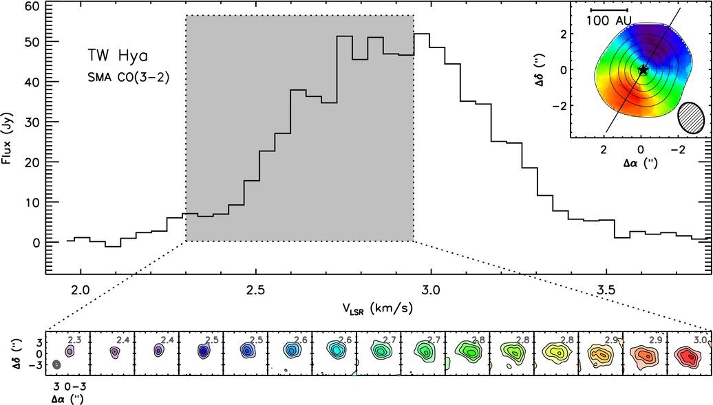
HCO+(4-3) data has not previously been published, but SMA HCO+(3-2) data (at 267.55762 GHz) is presented in Qi et al. 2008 (ApJ, 681, 1396). These SMA data have comparable angular resolution but a wider 203 kHz channel width.

ALMA HCO+(4-3) moment maps from TW Hya, with white continuum contours at 3 and 100 sigma. From left to right: integrated intensity, intensity weighted velocity field, intensity weighted velocity dispersion are shown.
Obtaining the Data
We have provided the data for you on the tutorial computers. The calibration and imaging portions of the guide will step you through how to get started.
Once you return to your home institution, you may want to follow the full version of the CASA guide. In this case the data are available via the ALMA science portal here .
TWHya Data Reduction Tutorial
The tutorial has two main parts. We will spend the morning on calibration of the data and then the afternoon imaging the calibrated data (and using these images to further refine the calibration). There is a separate page for each part of the tutorial:
- TWHydraBand7_SS12 this page steps you through the morning calibration tutorial.
- TwHydraBand7_Imaging_SS12 this page steps you through the afternoon imaging and self-calibration tutorial.
How to Use A CASA guide
In the guides
# In CASA
Regions of this color are CASA commands (or definitions) that need to be cut and
pasted in sequence. Wait until one command is finished before pasting another.
Tabs matter in python, make sure that commands that span more than one line and
"for" loops keep their spacing. Sometimes (especially "for" loops) you may need to
explicitly hit enter twice to get the command going.
Information in this color shows excerpts from the CASA Logger output
This color shows you background information about the data or other types of reference material
This color shows summer-school-specific notes.
A few tips on using CASA (copied from the EVLA IRC+10216 tutorial):

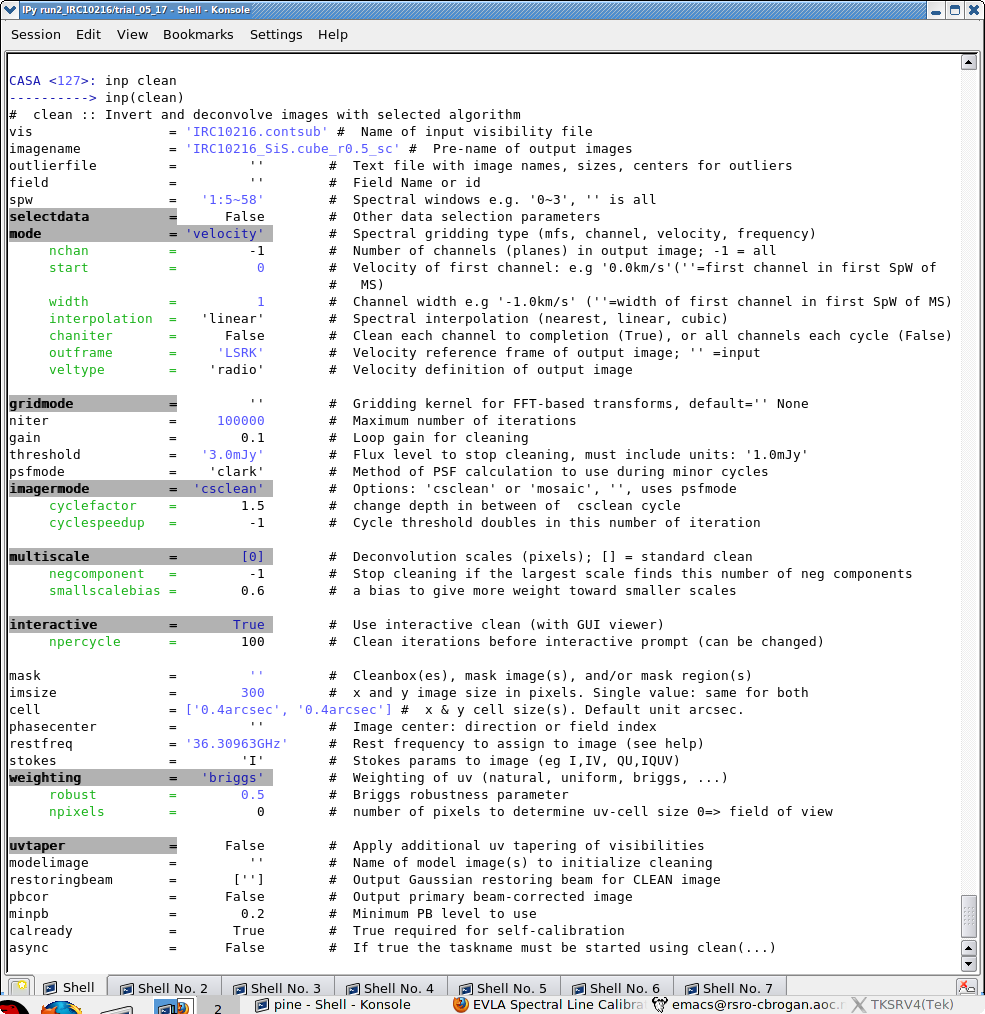
There are a number of possible ways to run CASA. Many aspects are described in Getting_Started_in_CASA. You should review this page if you are new to CASA. In brief you can run CASA interactively by looking at the inputs to tasks with inp taskname (example: inp clean), setting the parameters one by one (example: selectdata=T) as you desire and then run go. After setting parameters one by one in a task and then looking at the inputs again, you will notice that the parameters that have been set to something other than their defaults are blue. If you have mistyped any parameters, they will be red and must be fixed for the task to run correctly. You can get more detailed help on any task by typing help taskname (example: help clean). Once a task is run you can get the same parameters back by running tget taskname (example: tget clean); subsequent runs will overwrite the previous tget file.
The second way to run CASA is to provide task function calls. This tutorial is made up of such calls, which were developed by looking at the inputs for each task and deciding what needed to be changed from default values. For task function calls, only parameters that you want to be different from their defaults need to be set. A series of task function calls can be combined together into a script, and run with execfile('scriptname.py'). It is possible to extract a script containing all the CASA task function calls in this and other casaguides using the method described at the Extracting_scripts_from_these_tutorials page.
If you are a relative novice or just new to CASA it is strongly recommended to work through this tutorial by cutting and pasting the task function calls provided below after you have read all the associated explanations. Work at your own pace, look at the inputs to the tasks to see what other options exist, and read the help files. Later, when you are more comfortable, you might try to extract the script, modify it for your purposes, and begin to reduce other data.