PPdisk simdata (CASA 3.2): Difference between revisions
From CASA Guides
Jump to navigationJump to search
| (9 intermediate revisions by 2 users not shown) | |||
| Line 1: | Line 1: | ||
{{Simulations Intro}} | {{Simulations Intro}} | ||
[[Category: Simulations]] | [[Category: Simulations]] | ||
''A new version of this page exists for CASA 3.3: [[PPdisk simdata (CASA 3.3)]].'' | |||
== Protoplanetary disk == | == Protoplanetary disk == | ||
| Line 49: | Line 51: | ||
totaltime = "1200s" | totaltime = "1200s" | ||
=====Use appropriate antenna configurations based on desired angular resolution===== | =====Use appropriate antenna configurations based on desired angular resolution (configuration 20 is the largest "compact" configuration)===== | ||
repodir=os.getenv("CASAPATH").split(' ')[0] | repodir=os.getenv("CASAPATH").split(' ')[0] | ||
antennalist = repodir+"/data/alma/simmos/alma.out20.cfg" | antennalist = repodir+"/data/alma/simmos/alma.out20.cfg" | ||
=====Deconvolve the visibilities back into an image===== | =====Deconvolve the visibilities back into an image===== | ||
image = True | image = True | ||
| Line 70: | Line 73: | ||
overwrite = True | overwrite = True | ||
=== | ===Run simdata=== | ||
CASA<> go simdata | CASA<> go simdata | ||
| Line 82: | Line 83: | ||
{| style="border:1px solid #3366FF; " cellspacing=2 | {| style="border:1px solid #3366FF; " cellspacing=2 | ||
|Input:<br> [[File:Psim2.skymodel.png|300px]] | |Input:<br> [[File:Psim2.skymodel.png|300px]] | ||
|Predict:<br> [[File:Psim2. | |Predict:<br> [[File:Psim2.observe.png|300px]] | ||
|- | |- | ||
|Image:<br> [[File:Psim2.image.png|300px]] | |Image:<br> [[File:Psim2.image.png|300px]] | ||
|Analyze:<br> [[File:Psim2.analysis.png|300px]] | |Analyze:<br> [[File:Psim2.analysis.png|300px]] | ||
|} | |} | ||
{{Simulations Intro}} | |||
Latest revision as of 20:27, 3 November 2011
↵ Simulating Observations in CASA
A new version of this page exists for CASA 3.3: PPdisk simdata (CASA 3.3).
Protoplanetary disk
- This fits file is a model of a protoplanetary disk from S. Wolf (If you use it for anything more than learning CASA, please cite Wolf & D'Angelo 2005).
- Simdata version for CASA 3.2
Explanation of the script
Set simdata as current task and reset all parameters
default("simdata")
Specify sky model image
modelimage = "input50pc_672GHz.fits"
Image coordinate system can be verified
imhead("input50pc_672GHz.fits")
Image center can be identified
 # ia.open("input50pc_672GHz.fits")
 # ia.shape()
 # [257L, 257L, 1L, 1L]
 # ia.toworld([128.5,128.5])
 # {'numeric': array([  4.71239120e+00,  -4.01423802e-01,   1.00000000e+00,  6.72000001e+11])}
 # qa.formxxx("4.71239120rad",format='hms',prec=5)
 # '18:00:00.03052'
 # qa.formxxx("-0.401423802rad",format='dms',prec=5)
 # '-022.59.59.602743'
 # ia.done()
Brightness scale can be viewed with 'imstat' task
imstat("input50pc_672GHz.fits")
# ...
#  'max': array([  6.52469971e-05]),
# ...
# that's 0.0652 mJy/pixel.
Let's call our project psim2
project = "psim2"
We'll leave the sky model the way it is: simdata will create psim2.skymodel CASA image since this model is a fits file, and most but not all of CASA routines can operate directly on fits
modifymodel        =  False
skymodel           =  "input50pc_672GHz.fits"
We need to decide where to point the telescope. The image is 2/3 arcsec in size, so we only need one pointing. We could put that in a text file ourself, or let simdata create the ascii pointing file for us.
setpointings       =  True
direction          =  "J2000 18h00m00.031s -22d59m59.6s"
mapsize            =  "0.76arcsec"
The default pointingspacing is fine: we'll only fit one pointing in the small mapsize the default calculation maptype hexagonal is ok too since only one will fit anyway.
We do want to calculate visibilities in a measurement set: let's do a 20 min snapshot observation using out20 configuration:
predict            =  True
totaltime          =  "1200s"
Use appropriate antenna configurations based on desired angular resolution (configuration 20 is the largest "compact" configuration)
repodir=os.getenv("CASAPATH").split(' ')[0]
antennalist        =  repodir+"/data/alma/simmos/alma.out20.cfg"
Deconvolve the visibilities back into an image
image              =  True
vis                =  "$project.ms"
imsize             =  [192, 192]
Specify number of iteration of cleaning task with proper threshold and weighting
niter              =  10000
threshold          =  "1e-7Jy"
weighting          =  "natural"
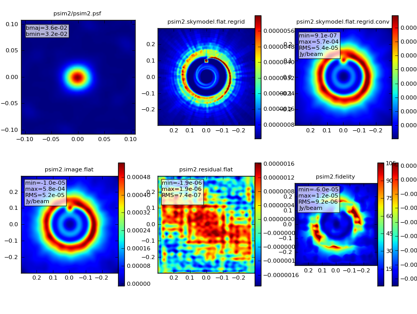
We'd like to calculate a difference and fidelity image, and see some diagnostics:
analyze = True
And see the array but not the UV coverage:
showarray          =  True
showuv             =  False
Plot both to the screen and the png files with lots of messages:
graphics           =  "both"
verbose            =  True
overwrite = True
Run simdata
CASA<> go simdata
- Output results:
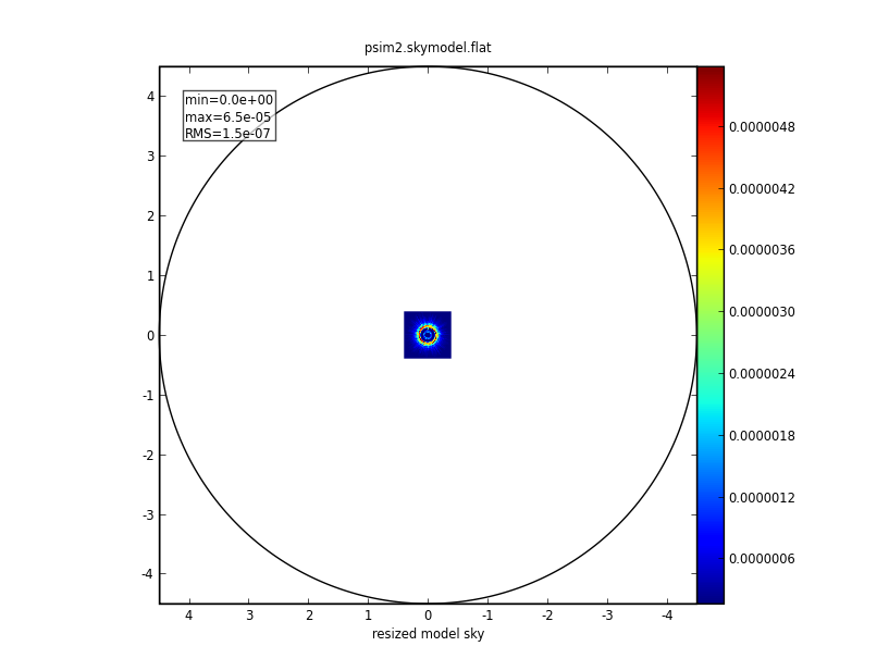
Input:
|
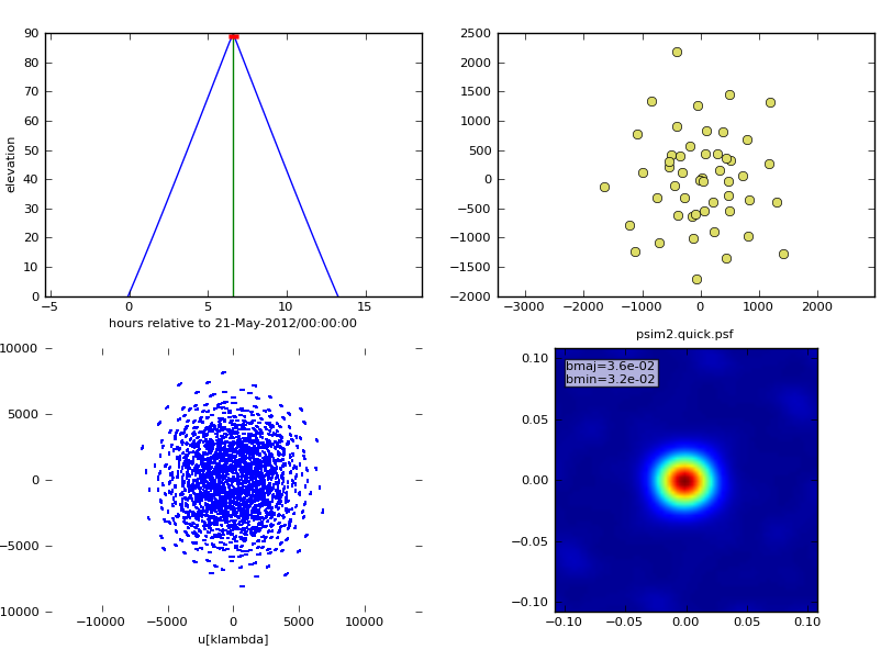
Predict:
|
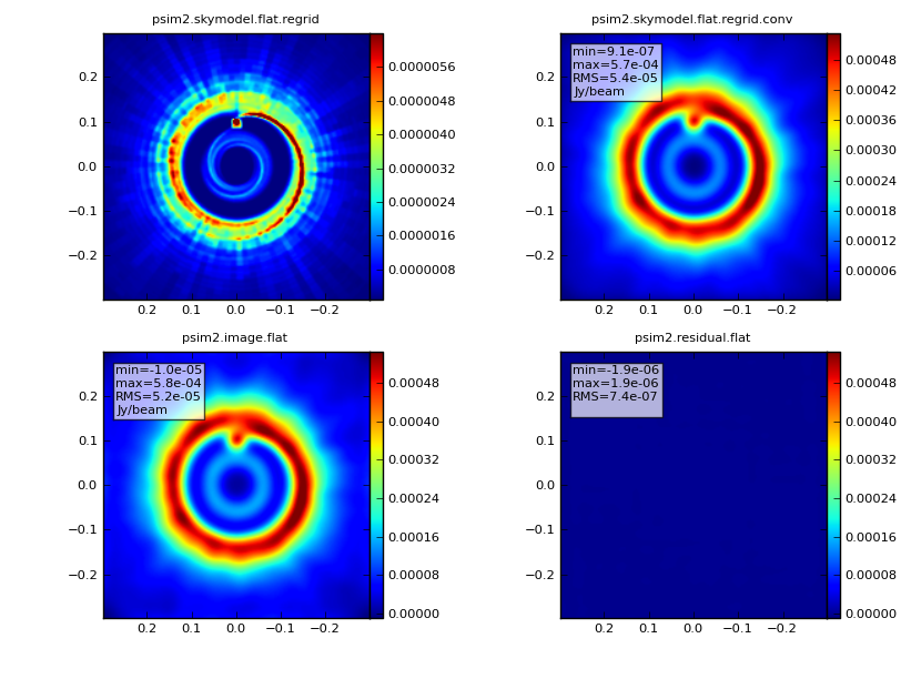
Image:
|
Analyze:
|