EVLA Spectral Line Imaging Analysis IRC+10216: Difference between revisions
No edit summary |
|||
| (53 intermediate revisions by 4 users not shown) | |||
| Line 1: | Line 1: | ||
This tutorial picks up where [[EVLA Spectral Line Calibration IRC+10216]] leaves off. | This tutorial picks up where [[EVLA Spectral Line Calibration IRC+10216]] leaves off. | ||
| Line 16: | Line 9: | ||
plotms(vis='IRC10216',field='',ydatacolumn='corrected', | plotms(vis='IRC10216',field='',ydatacolumn='corrected', | ||
xaxis='channel',yaxis='amp',correlation='RR', | xaxis='channel',yaxis='amp',correlation='RR', | ||
avgtime='1e8',avgscan=T,spw='0~1:4~60',antenna='') | avgtime='1e8',avgscan=T,spw='0~1:4~60',antenna='', coloraxis='spw') | ||
</source> | </source> | ||
in the Display tab, | in the Display tab, change the Unflagged points symbol to custom and Style of 3. | ||
You should see the "horned profile" typical of a rotation shell. From this plot, you can guess that strong | You should see the "horned profile" typical of a rotation shell. From this plot, you can guess that strong | ||
| Line 35: | Line 28: | ||
The "want_cont=T" will produce two new datasets, IRC10216.contsub is the continuum subtracted line data, and IRC10216.cont is the continuum estimate (note however, that it is still a multi-channel dataset). | The "want_cont=T" will produce two new datasets, IRC10216.contsub is the continuum subtracted line data, and IRC10216.cont is the continuum estimate (note however, that it is still a multi-channel dataset). | ||
'''If you want to try self-cal:''' Unfortunately, at the moment, uvcontsub2 doesn't leave the continuum subtracted line dataset in the state you need *if* you think you might want to self-calibrate the data later. This is because | <!-- | ||
'''If you want to try self-cal:''' Unfortunately, at the moment, uvcontsub2 doesn't leave the continuum subtracted line dataset in the state you need *if* you think you might want to self-calibrate the data later. This is because {{clean}} always looks at the "corrected" datacolumn, while {{gaincal}} (also used for self-calibration) always looks at the "data" column. You also need to know that unless the imagename supplied to clean already exists, clean always overwrites the model column with the clean model (this will be the model supplied to the self-calibration process). | |||
<pre style="background-color: #E0FFFF;"> | <pre style="background-color: #E0FFFF;"> | ||
The files produced by uvcontsub2 will have the following in their data columns: | The files produced by uvcontsub2 will have the following in their data columns: | ||
| Line 43: | Line 37: | ||
</pre> | </pre> | ||
Now the imaging task | Now the imaging task {{clean}} will clean both of these files fine, and correctly overwrite the model data column with the correct clean model. However, if you try to self-cal (i.e. run gaincal) on the continuum subtracted line data (.contsub), it will use the Line+Cont as its input along with the line only clean model. If the line and continuum have significantly different morphology (almost always) the self-cal process will fail. In contrast the continuum dataset (.cont) will work fine because the Data and Corrected columns agree. | ||
To fix things up, we must | To fix things up, we must {{split}} the "corrected" column (which places "Corrected" in the "Data" column of the new dataset. Then you can either run clearcal to reinitialize the "model" and "corrected" columns or let clean do it for you. We put this step here explicitly for clarity about the process. | ||
<source lang="python"> | <source lang="python"> | ||
| Line 54: | Line 48: | ||
</source> | </source> | ||
Now IRC10216.contsub.data will have the Line in the "data" column, 1 in the "model" column, and the Line in the "corrected" column as desired. | Now IRC10216.contsub.data will have the Line in the "data" column, 1 in the "model" column for amplitudes and 0 for phase, and the Line in the "corrected" column as desired. You can always check this using {{plotms}} to | ||
look at the "data", "model", and "corrected" columns. | |||
We expect that these extra shenanigans will be unnecessary in the future. | We expect that these extra shenanigans will be unnecessary in the future. | ||
--> | |||
==Image the Spectral Line Data== | ==Image the Spectral Line Data== | ||
| Line 68: | Line 65: | ||
<source lang="python"> | <source lang="python"> | ||
# In CASA | # In CASA | ||
clean(vis='IRC10216.contsub' | clean(vis='IRC10216.contsub',imagename='IRC10216_HC3N.cube_r0.5', | ||
imagermode='csclean', | imagermode='csclean', | ||
imsize=300,cell=['0.4arcsec'],spw='0:5~58', | imsize=300,cell=['0.4arcsec'],spw='0:5~58', | ||
| Line 78: | Line 75: | ||
</source> | </source> | ||
It will take a little while to grid the data, but the | It will take a little while to grid the data, but the {{viewer}} will open when it's ready to start an interactive clean. Use the "tape deck" at the bottom of the Viewer display GUI to step through to the channel with the most extended (in angular size) emission, select "all channels" for the clean mask, select the polygon tool (second in from the right) and make a single mask that applies to all channels (see example in thumbnail). Once you make the polygon region, you need to double click inside it to save the mask region -- if you see the polygon turn white you will know you succeeded. Note, that if you had the time and patience you could make a clean mask for each channel, and this would create a slightly better result. | ||
After making the mask you should check that the emission in all the other channels fits within the mask you made using the "tape deck" to move back and forth. If you need to include more area in the mask, you can chose the "erase" toggle at the top, and then encircle your existing mask with a polygon and double click inside. Then go back to "add" toggle at top and make a new mask. Alternatively, you can erase a part of the mask, or you can add to the existing mask by drawing new polygons. Feel free to experiment with this a bit. | After making the mask you should check that the emission in all the other channels fits within the mask you made using the "tape deck" to move back and forth. If you need to include more area in the mask, you can chose the "erase" toggle at the top, and then encircle your existing mask with a polygon and double click inside. Then go back to "add" toggle at top and make a new mask. Alternatively, you can erase a part of the mask, or you can add to the existing mask by drawing new polygons. Feel free to experiment with this a bit. | ||
| Line 84: | Line 81: | ||
'''note''': If you start an interactive clean, and then do not make a mask, clean will stop when you tell it to go on because it has nothing to clean. There is no default mask. | '''note''': If you start an interactive clean, and then do not make a mask, clean will stop when you tell it to go on because it has nothing to clean. There is no default mask. | ||
To continue with | To continue with {{clean}} use the "Next action" buttons in the green area on the Viewer Display GUI: The red X will stop {{clean}} where you are, the blue arrow will stop the interactive part of {{clean}}, but continue to clean non-interactively until reaching the stopping niter or threshold (whichever comes first), and the green arrow will clean until it reaches the "iterations" parameter on the left side of the green area. When | ||
the interactive viewer comes back use the tape deck to recheck that | the interactive viewer comes back use the tape deck to recheck that your mask encompasses what you think is real emission. The middle mouse button by default controls the image stretch. | ||
Note that for this example, threshold has been set to threshold='3mJy' to protect you from cleaning too deeply. With a careful clean mask you can clean to close to the thermal noise limit (note here I mean the actual observed rms noise limit and not the theoretical one you calculated for the proposal, as flagging, weather etc can affect what you actually get). It is ALWAYS best to clean each channel in a cube to a specific threshold than to stop using the niter parameter, which can leave each channel cleaned to different levels. There are many ways to determine a suitable threshold. One way is to make a dirty image (niter=0), open the cube using the viewer, go to a line free channel, select the box region tool, make a box near the field center about the size of your source, double click inside. The rms noise of that channel will appear in a pop-up window (rms noise for whole cube will go to terminal). Try a few different boxes, average the results and this is a good estimate of the rms per channel assuming your data are not dynamic range limited (i.e. noise can be higher in channels with strong signal). This is the absolute minimum for threshold. With no mask you probably shouldn't clean deeper than 3x this rms. | Note that for this example, threshold has been set to threshold='3mJy' to protect you from cleaning too deeply. With a careful clean mask you can clean to close to the thermal noise limit (note here I mean the actual observed rms noise limit and not the theoretical one you calculated for the proposal, as flagging, weather etc can affect what you actually get). It is ALWAYS best to clean each channel in a cube to a specific threshold than to stop by simply using the niter parameter, which can leave each channel cleaned to different levels. There are many ways to determine a suitable threshold. One way is to make a dirty image (niter=0), open the cube using the viewer, go to a line free channel, select the box region tool, make a box near the field center about the size of your source, and double click inside. The rms noise of that channel will appear in a pop-up window (rms noise for whole cube will go to terminal). Try a few different boxes, average the results and this is a good estimate of the rms per channel assuming your data are not dynamic range limited (i.e. noise can be higher in channels with strong signal). This is the absolute minimum for threshold. With no mask you probably shouldn't clean deeper than 3x this rms. | ||
[[Image:SiS_interactive.png|thumb|Channel 16 shown for the SiS cube in the interactive viewer with the white contour showing the mask contour drawn with the polygon tool.]] | [[Image:SiS_interactive.png|thumb|Channel 16 shown for the SiS cube in the interactive viewer with the white contour showing the mask contour drawn with the polygon tool.]] | ||
| Line 97: | Line 94: | ||
<source lang="python"> | <source lang="python"> | ||
# In CASA | # In CASA | ||
clean(vis='IRC10216.contsub | clean(vis='IRC10216.contsub',imagename='IRC10216_SiS.cube_r0.5', | ||
imagermode='csclean', | imagermode='csclean', | ||
imsize=300,cell=['0.4arcsec'],spw='1:5~58', | imsize=300,cell=['0.4arcsec'],spw='1:5~58', | ||
| Line 105: | Line 102: | ||
interactive=T, | interactive=T, | ||
threshold='3.0mJy',niter=100000) | threshold='3.0mJy',niter=100000) | ||
</source> | |||
You can look at both cubes using the viewer, and the tape deck to play the cube as "movie". | |||
<source lang="python"> | |||
# In CASA | |||
viewer | |||
</source> | </source> | ||
==Image the Continuum data== | ==Image the Continuum data== | ||
Below the use of mode='mfs' will make a single multi-frequency synthesis image out of the specified spw. Again you should make an interactive clean mask. Since no threshold is set, you will need to stop cleaning when the residual looks noise like using the red x "Next Action" button (it will be done when the viewer comes back the second time). | Below the use of mode='mfs' will make a single multi-frequency synthesis image out of the specified spw/channels. Again you should make an interactive clean mask. Since no threshold is set, you will need to stop cleaning when the residual looks noise like using the red x "Next Action" button (it will be done when the viewer comes back the second time). The continuum for IRC10216 is very weak but interesting -- it is essentially tracing the photosphere of the AGB star. | ||
<source lang="python"> | <source lang="python"> | ||
| Line 124: | Line 127: | ||
<source lang="python"> | <source lang="python"> | ||
# In CASA | # In CASA | ||
viewer | |||
</source> | </source> | ||
| Line 138: | Line 141: | ||
Then use the Viewer tape deck to see which channels have significant line emission. For HC3N, the line channel range in the cube is 11 to 40, and it is the same for SiS. | Then use the Viewer tape deck to see which channels have significant line emission. For HC3N, the line channel range in the cube is 11 to 40, and it is the same for SiS. | ||
Then use the tape deck to go to a line free channel, select the box region tool and make a box. When you double click in the box, the image statistics | [[Image:irc10216.jpg|thumb|HC3N moment 0 map with white continuum contours superposed.]] | ||
[[Image:irc10216_sismom0.jpg|thumb|SiS moment 0 map with white continuum contours superposed.]] | |||
Then use the tape deck to go to a line free channel, select the box region tool and make a box. When you double click in the box, the image statistics for the channel you are on will print to the terminal. Move the box around a bit to see what the variation in rms noise is. You should get something like 2 mJy. Note that the rms is much worse in channels with strong emission because of the low dynamic range of these data. If you want the box tool to go away (i.e. if you want to make a new one), hit the escape key. | |||
Now lets make the moment 0 and moment 1 maps. For moment zero, | Now lets make the moment 0 and moment 1 maps. For moment zero, it's best to limit the calculation to image channels with significant signal in them, but not to apply a flux cutoff, as this will bias the derived integrated intensities upward. | ||
<source lang="python"> | <source lang="python"> | ||
# In CASA | # In CASA | ||
| Line 161: | Line 165: | ||
For moment 1, it is essential to apply a conservative flux cutoff to limit the calculation to high signal-to-noise areas. Here we use about 5sigma. | For moment 1, it is essential to apply a conservative flux cutoff to limit the calculation to high signal-to-noise areas. Here we use about 5sigma. | ||
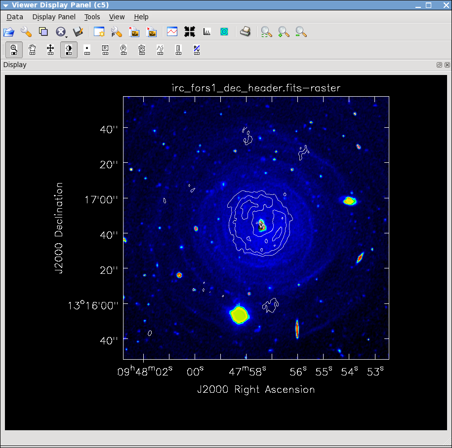
[[Image:irc10216_dust_HC3N_cont.png|thumb|The VLT V-band image from Leão et al. (2006, A&A, 455,187) showing dust rings, overlaid with white HC3N moment 0 contours and black 36 GHz continuum contours.]] | |||
<source lang="python"> | <source lang="python"> | ||
| Line 178: | Line 184: | ||
</source> | </source> | ||
Now | |||
Now use the viewer to further explore the images you've made. | |||
For fun you can download the VLT V-band image at http://casa.nrao.edu/Data/EVLA/IRC10216/irc_fors1_dec_header.fits kindly provided by | |||
Izan Leão and overlay the moment images and 36 GHz continuum. More information about the dust properties can be found in the Leão et al. (2006) paper http://adsabs.harvard.edu/abs/2006A%26A...455..187L | |||
== Self-Calibration == | == Self-Calibration == | ||
| Line 184: | Line 194: | ||
The many different aspects of self-calibration could fill several casaguides. Here we describe a simple process for this particular relatively low S/N data (low S/N per channel at least). | The many different aspects of self-calibration could fill several casaguides. Here we describe a simple process for this particular relatively low S/N data (low S/N per channel at least). | ||
While running | While running {{clean}} above, the model column for each channel will have been filled with the clean model (if you made a Fourier transform of this model, you would see an image of the clean components). | ||
We chose to do the self cal on the spw=1 SiS line data because it has the strongest emission in a single channel and is a bit more compact than the HC3N data. We will run | We chose to do the self cal on the spw=1 SiS line data because it has the strongest emission in a single channel and is a bit more compact than the HC3N data. We will run {{gaincal}} specifying the channel in the uv-data that has the brightest peak in the image (use the {{viewer}} to figure out which channel this is for spw=1), note down what the peak flux is. Since we started the image with a channel range we need to account for the fact that the image channel numbers do not map exactly to the uv-data channel numbers (they are off by 5 so that channel 13 in the image is roughly channel 19 in the uv-data). | ||
The next thing we need to understand is the S/N of the data. In particular, to self-cal, you need enough signal on a single baseline over the course of your chosen solint to get a S/N of about 3. Above we calculated an average rms noise of about 2 mJy/beam/channel for the whole timerange (about 95 minutes on source time) and all antennas (16). We can use our knowledge of the radiometer equation (see [http://evlaguides.nrao.edu/index.php?title=Category:Status#Sensitivity EVLA Sensitivity]) where rms scales as 1/sqrt(time * #baselines), and the number of baselines= N(N-1)/2 and N=# of antennas. So the rms noise on one baseline, one 10 second integration is given by: | |||
<math> {\rm RMS(baseline)} = {\rm 2\ mJy\ beam^{-1}\ channel^{-1}} \sqrt{ \frac{95\times 60\ {\rm sec}}{10\ {\rm sec}}\times\frac{16\times 15}{2\times 1}}</math> | |||
[[Image:timeonsource.png|thumb|Plot to estimate the time on source.]] | |||
The 95 minutes of on-source time can be estimated from a plot like: | |||
<source lang="python"> | <source lang="python"> | ||
# In CASA | # In CASA | ||
plotms(vis='day2_TDEM0003_10s_norx',field='3',ydatacolumn='corrected', | |||
xaxis='time',yaxis='amp',correlation='RR,LL', | |||
avgchannel='64',spw='1:4~60',antenna='') | |||
</source> | </source> | ||
This analysis suggests that the rms noise on one baseline, one 10 second integration is about 525 mJy. In contrast the peak flux density in the strongest SiS channel is only about 200 mJy (you can check using the {{viewer}}). Because the emission is fairly compact, most baselines will see about this peak flux, this is why we chose the more compact of the two possible lines. This peak flux density tells us that we need to use a solint large enough so that the rms noise is not worse than about 1/3 of 200 mJy. Thus, a solint of 10 minutes is about the shortest we can use and be reasonably confident of the solutions. | |||
Now we run {{gaincal}} with the solint we have determined. Note that because our desired solint is more | |||
than the scan time, we need to include combine='scan'. | |||
<source lang="python"> | <source lang="python"> | ||
# In CASA | # In CASA | ||
gaincal(vis='IRC10216.contsub | gaincal(vis='IRC10216.contsub',caltable='pcal_ch19one_10min', | ||
spw='1:19~19',calmode='p',solint=' | spw='1:19~19',calmode='p',solint='10min',combine='scan', | ||
refant='ea02',minsnr= | refant='ea02',minsnr=3.0) | ||
</source> | |||
[[Image:selfcalone.png|thumb|Phase-only self-calibration solutions with 10 minute solint.]] | |||
Now let's look at the solutions: | |||
<source lang="python"> | <source lang="python"> | ||
# In CASA | # In CASA | ||
plotcal(caltable=' | plotcal(caltable='pcal_ch19one_10min',xaxis='time',yaxis='phase', | ||
iteration='antenna',subplot=331,plotrange=[0,0,-50,50]) | iteration='antenna',subplot=331,plotrange=[0,0,-50,50]) | ||
</source> | </source> | ||
For some antennas you can see clear global trends away from zero: ea08, ea21,ea24 are examples, and you can also see some smaller variations with time. | |||
Now let's explore whether applying this solution actually improves matters. To do this we need to run {{applycal}} to apply the solutions to the line dataset, both spw. We need to use spwmap to tell it that the solutions derived for spw=1 should be applied to both spw=0 and spw=1. Again it's important to set calwt=F here. | |||
<source lang="python"> | <source lang="python"> | ||
# In CASA | # In CASA | ||
applycal(vis='IRC10216.contsub',field='',spw='0,1', | |||
gaintable=['pcal_ch19one_10min'],spwmap=[[1,1]],calwt=F) | |||
</source> | |||
'''Note:''' in this example we ran the self-cal steps on the full uv continuum subtracted spectral line data set. For a more complex iterative self-calibration proceedure, you may find it easier to split off the channel/spw you want to experiment on with {{split}}, and then do all the imaging ({{clean}}) and {{gaincal}} steps with it. The {{gaincal}} tables created on the single channel can still be applied with {{applycal}} to the multi-channel/spw dataset. If you do this though, keep in mind that once split, the single-channel data will have its spw id reset to 0 (you can check with {{listobs}}), no matter what spw it came from. Thus in order to applycal with it you would need <nowiki>spwmap=[[0,0]]</nowiki>. | |||
To save time we can use the clean mask we made before and run in a non-interactive mode. You can use a mask over again as long as the number of channels in the {{clean}} call haven't changed. You can change cell or imsize and it will still do the right thing. | |||
<source lang="python"> | |||
# In CASA | |||
clean(vis='IRC10216.contsub',imagename='IRC10216_HC3N.cube_r0.5.pselfcal', | |||
imagermode='csclean', | |||
imsize=300,cell=['0.4arcsec'],spw='0:5~58', | |||
mode='velocity',interpolation='linear', | |||
restfreq='36.39232GHz',outframe='LSRK', | |||
weighting='briggs',robust=0.5, | |||
mask='IRC10216_HC3N.cube_r0.5.mask', | |||
interactive=F,threshold='3.0mJy',niter=100000) | |||
</source> | </source> | ||
<source lang="python"> | |||
# In CASA | |||
clean(vis='IRC10216.contsub',imagename='IRC10216_SiS.cube_r0.5.pselfcal', | |||
imagermode='csclean',calready=T, | |||
imsize=300,cell=['0.4arcsec'],spw='1:5~58', | |||
mode='velocity',interpolation='linear', | |||
restfreq='36.30963GHz',outframe='LSRK', | |||
weighting='briggs',robust=0.5, | |||
mask='IRC10216_SiS.cube_r0.5.mask', | |||
interactive=F,threshold='3.0mJy',niter=100000) | |||
</source> | |||
Now investigate the original and self-cal'ed images in the viewer. You will find that even this single self-cal step significantly improves the images. Try opening both versions of the SiS image cubes. | |||
Then select a bright channel from the tape deck like channel 37, then use the "wrench" and "pwrench" guis to make a plot like below setting the same image range for both cubes, and two panels in x, then to see both images of that channel side-by-side click the blink toggle (see image below for more tips on setup.) | |||
[[Image:compareselfcal.png|600px|Original and self-cal SiS images for channel 37, notice the decrease in | |||
residuals.]] | |||
Repeat for HC3N: | |||
[[Image:compareselfcal2.png|600px|Original and self-cal HC3N images for channel 13, notice the decrease in | |||
residuals.]] | |||
Now you can redo the moment images if you like with the improved cubes, be sure to change the output file names. | |||
[[Main Page | ↵ '''CASAguides''']] | [[Main Page | ↵ '''CASAguides''']] | ||
--[[User:Cbrogan|Crystal Brogan]] | --[[User:Cbrogan|Crystal Brogan]] | ||
{{Checked 3.2.0}} | |||
Latest revision as of 20:03, 2 September 2011
This tutorial picks up where EVLA Spectral Line Calibration IRC+10216 leaves off.
UV Continuum Subtraction and Setting Up for Self-Calibration
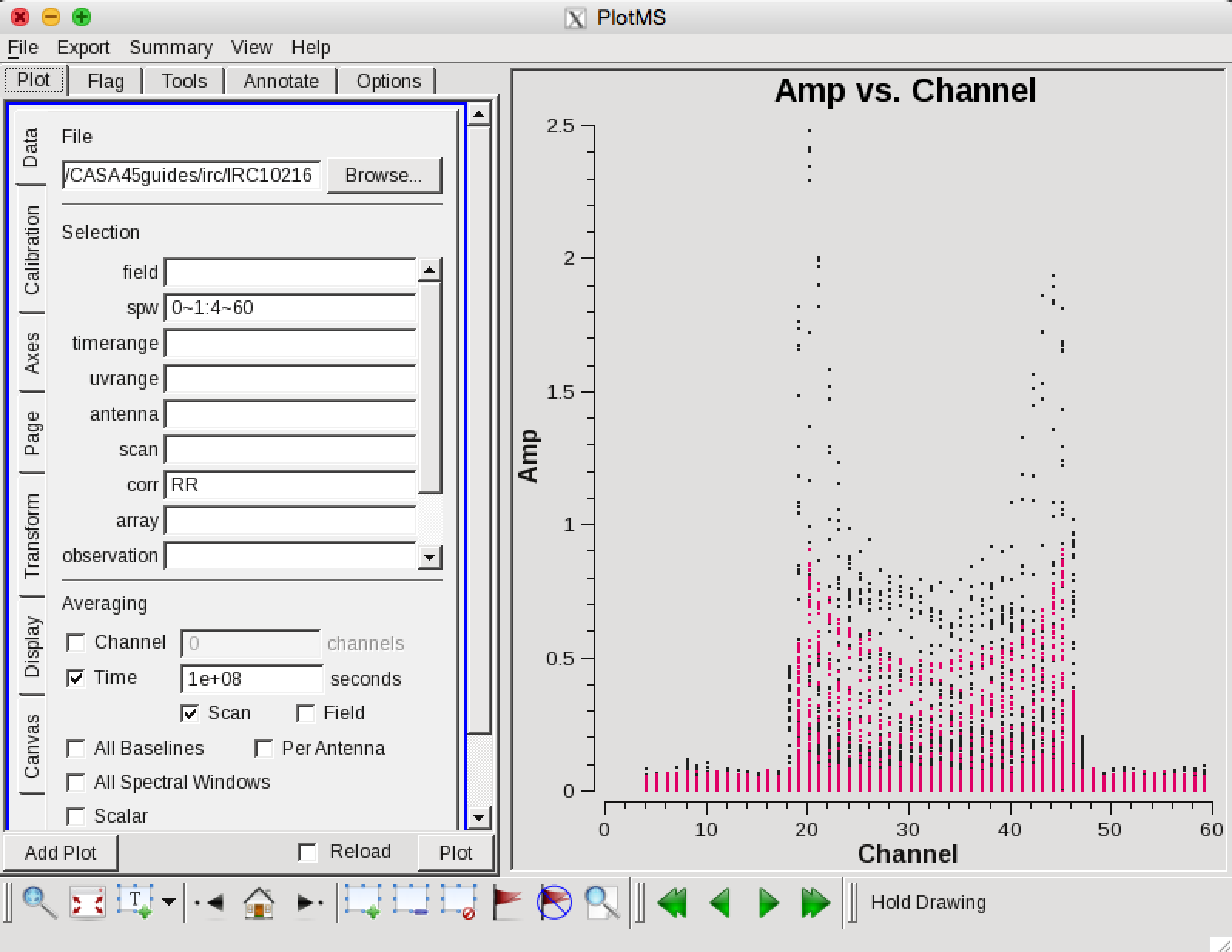
Now we can make a vector averaged uv-plot of the calibrated target spectral line data. It is important to note that you will only see signal in such a plot if (1) the data are well calibrated, and (2) there is significant signal near the phase center of the observations, or if the line emission (or absorption) is weak but extended. If this isn't true for your data, you won't be able to see the line signal in such a plot and will need to make an initial (dirty or lightly cleaned) line+continuum cube to determine the line-free channels. Generally, this is the recommended course for finding the line-free channels more precisely than is being done here due to time constraints, as weak line signal would not be obvious in this plot.
plotms(vis='IRC10216',field='',ydatacolumn='corrected',
       xaxis='channel',yaxis='amp',correlation='RR',
       avgtime='1e8',avgscan=T,spw='0~1:4~60',antenna='', coloraxis='spw')
in the Display tab, change the Unflagged points symbol to custom and Style of 3.
You should see the "horned profile" typical of a rotation shell. From this plot, you can guess that strong line emission is restricted to channels 18 to 47 (zoom in if necessary to see exactly what the channel numbers are).
In the Data tab you can also click on "all baselines" to average all baselines, but this is a little harder to see.
Now we want to use the line free channels to create a model of the continuum emission that can be subtracted to form a line-only dataset. We want to refrain from going to close to the edges of the band -- these channels are typically noisy, and we don't want to get too close to the line channels because we could only see strong line emission in the vector averaged uv-plot.
uvcontsub2(vis='IRC10216',fitspw='0~1:4~13;52~60',
       want_cont=T)
The "want_cont=T" will produce two new datasets, IRC10216.contsub is the continuum subtracted line data, and IRC10216.cont is the continuum estimate (note however, that it is still a multi-channel dataset).
Image the Spectral Line Data
Here we make images from the continuum-subtracted, calibrated spectral line data. Because the spectral line emission from IRC+10216 has significant extended emission, it is very important to run clean interactively, and make a clean mask. To make the cube a bit smaller and stay away from noisy edge channels we restrict the channel range using the spw parameter.
# In CASA
clean(vis='IRC10216.contsub',imagename='IRC10216_HC3N.cube_r0.5',
      imagermode='csclean',
      imsize=300,cell=['0.4arcsec'],spw='0:5~58',
      mode='velocity',interpolation='linear',
      restfreq='36.39232GHz',outframe='LSRK',
      weighting='briggs',robust=0.5,
      interactive=T,
      threshold='3.0mJy',niter=100000)
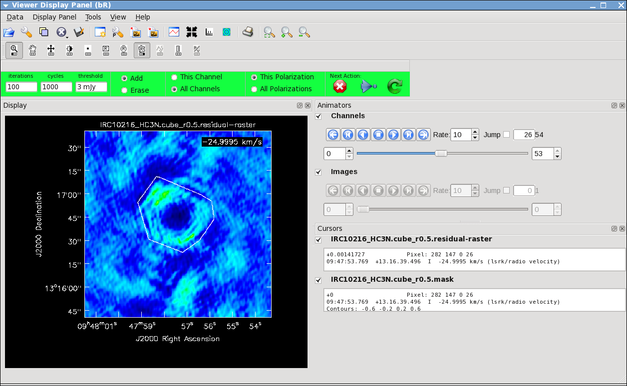
It will take a little while to grid the data, but the viewer will open when it's ready to start an interactive clean. Use the "tape deck" at the bottom of the Viewer display GUI to step through to the channel with the most extended (in angular size) emission, select "all channels" for the clean mask, select the polygon tool (second in from the right) and make a single mask that applies to all channels (see example in thumbnail). Once you make the polygon region, you need to double click inside it to save the mask region -- if you see the polygon turn white you will know you succeeded. Note, that if you had the time and patience you could make a clean mask for each channel, and this would create a slightly better result.
After making the mask you should check that the emission in all the other channels fits within the mask you made using the "tape deck" to move back and forth. If you need to include more area in the mask, you can chose the "erase" toggle at the top, and then encircle your existing mask with a polygon and double click inside. Then go back to "add" toggle at top and make a new mask. Alternatively, you can erase a part of the mask, or you can add to the existing mask by drawing new polygons. Feel free to experiment with this a bit.
note: If you start an interactive clean, and then do not make a mask, clean will stop when you tell it to go on because it has nothing to clean. There is no default mask.
To continue with clean use the "Next action" buttons in the green area on the Viewer Display GUI: The red X will stop clean where you are, the blue arrow will stop the interactive part of clean, but continue to clean non-interactively until reaching the stopping niter or threshold (whichever comes first), and the green arrow will clean until it reaches the "iterations" parameter on the left side of the green area. When the interactive viewer comes back use the tape deck to recheck that your mask encompasses what you think is real emission. The middle mouse button by default controls the image stretch.
Note that for this example, threshold has been set to threshold='3mJy' to protect you from cleaning too deeply. With a careful clean mask you can clean to close to the thermal noise limit (note here I mean the actual observed rms noise limit and not the theoretical one you calculated for the proposal, as flagging, weather etc can affect what you actually get). It is ALWAYS best to clean each channel in a cube to a specific threshold than to stop by simply using the niter parameter, which can leave each channel cleaned to different levels. There are many ways to determine a suitable threshold. One way is to make a dirty image (niter=0), open the cube using the viewer, go to a line free channel, select the box region tool, make a box near the field center about the size of your source, and double click inside. The rms noise of that channel will appear in a pop-up window (rms noise for whole cube will go to terminal). Try a few different boxes, average the results and this is a good estimate of the rms per channel assuming your data are not dynamic range limited (i.e. noise can be higher in channels with strong signal). This is the absolute minimum for threshold. With no mask you probably shouldn't clean deeper than 3x this rms.
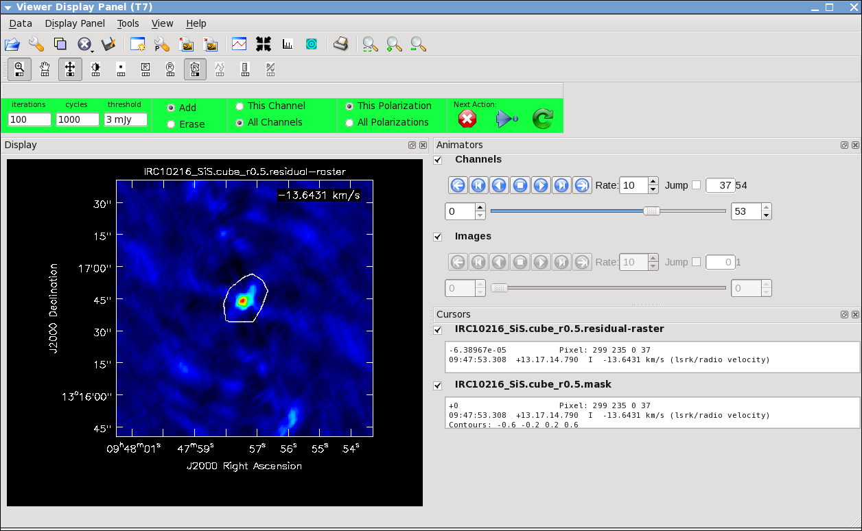
Keep cleaning, by using the green Next Action arrow until the residual displayed in the viewer looks "noise like". To speed things up, you might change the iteration parameter in the viewer to something like 300. This parameter can also be set in the task command. You will notice that in this particular case, there are residuals that cannot be cleaned -- these are due to the extended resolved out structure on size scales larger than the array is sensitive to (the "Largest Angular Scale" or LAS that the array is sensitive to can be calculated from the shortest baseline length), and potential residual phase and amplitude calibration errors. We will explore this in a few sections with self-calibration.
Repeat the process for the SiS line using the call below, note that the emission for this line is less extended than the HC3N -- this has to do with the different excitation requirements of the two different lines. The SiS is excited closer to the central star than the HC3N.
# In CASA
clean(vis='IRC10216.contsub',imagename='IRC10216_SiS.cube_r0.5',
      imagermode='csclean',
      imsize=300,cell=['0.4arcsec'],spw='1:5~58',
      mode='velocity',interpolation='linear',
      restfreq='36.30963GHz',outframe='LSRK',
      weighting='briggs',robust=0.5,
      interactive=T,
      threshold='3.0mJy',niter=100000)
You can look at both cubes using the viewer, and the tape deck to play the cube as "movie".
# In CASA
viewer
Image the Continuum data
Below the use of mode='mfs' will make a single multi-frequency synthesis image out of the specified spw/channels. Again you should make an interactive clean mask. Since no threshold is set, you will need to stop cleaning when the residual looks noise like using the red x "Next Action" button (it will be done when the viewer comes back the second time). The continuum for IRC10216 is very weak but interesting -- it is essentially tracing the photosphere of the AGB star.
# In CASA
clean(vis='IRC10216.cont',imagename='IRC10216.36GHzcont',
      mode='mfs',imagermode='csclean',
      imsize=300,cell=['0.4arcsec'],spw='0~1:5~59',
      weighting='briggs',robust=0.5,
      interactive=T)
Now look at the result in the viewer if you like
# In CASA
viewer
Image Analysis and Viewing
Next make integrated intensity maps (moment 0) and integrated velocity maps (moment 1). To do this, we'll want to know what channels the line emission starts and ends on, and also the rms noise in a single channel. So first lets open the viewer:
# In CASA
viewer
Then use the Viewer tape deck to see which channels have significant line emission. For HC3N, the line channel range in the cube is 11 to 40, and it is the same for SiS.
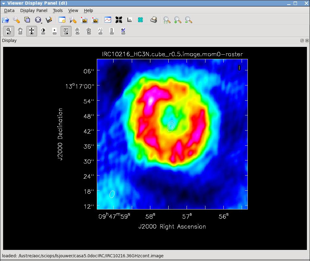
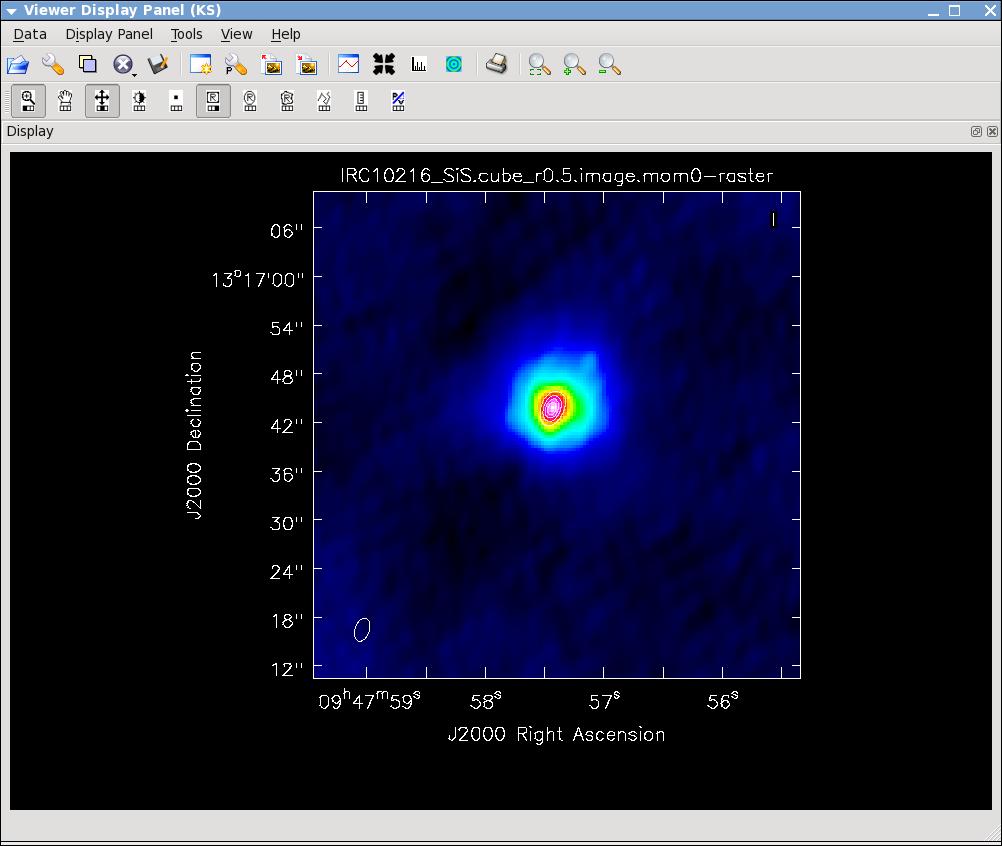
Then use the tape deck to go to a line free channel, select the box region tool and make a box. When you double click in the box, the image statistics for the channel you are on will print to the terminal. Move the box around a bit to see what the variation in rms noise is. You should get something like 2 mJy. Note that the rms is much worse in channels with strong emission because of the low dynamic range of these data. If you want the box tool to go away (i.e. if you want to make a new one), hit the escape key.
Now lets make the moment 0 and moment 1 maps. For moment zero, it's best to limit the calculation to image channels with significant signal in them, but not to apply a flux cutoff, as this will bias the derived integrated intensities upward.
# In CASA
immoments(imagename='IRC10216_HC3N.cube_r0.5.image',moments=[0],
          axis='spectral',
          chans='11~40',
          outfile='IRC10216_HC3N.cube_r0.5.image.mom0')
# In CASA
immoments(imagename='IRC10216_SiS.cube_r0.5.image',moments=[0],
          axis='spectral',
          chans='11~40',
          outfile='IRC10216_SiS.cube_r0.5.image.mom0')
For moment 1, it is essential to apply a conservative flux cutoff to limit the calculation to high signal-to-noise areas. Here we use about 5sigma.
# In CASA
immoments(imagename='IRC10216_HC3N.cube_r0.5.image',moments=[1],
          axis='spectral',
          chans='11~40',excludepix=[-100,0.01],
          outfile='IRC10216_HC3N.cube_r0.5.image.mom1')
# In CASA
immoments(imagename='IRC10216_SiS.cube_r0.5.image',moments=[1],
          axis='spectral',
          chans='11~40',excludepix=[-100,0.01],
          outfile='IRC10216_SiS.cube_r0.5.image.mom1')
Now use the viewer to further explore the images you've made.
For fun you can download the VLT V-band image at http://casa.nrao.edu/Data/EVLA/IRC10216/irc_fors1_dec_header.fits kindly provided by Izan Leão and overlay the moment images and 36 GHz continuum. More information about the dust properties can be found in the Leão et al. (2006) paper http://adsabs.harvard.edu/abs/2006A%26A...455..187L
Self-Calibration
The many different aspects of self-calibration could fill several casaguides. Here we describe a simple process for this particular relatively low S/N data (low S/N per channel at least).
While running clean above, the model column for each channel will have been filled with the clean model (if you made a Fourier transform of this model, you would see an image of the clean components).
We chose to do the self cal on the spw=1 SiS line data because it has the strongest emission in a single channel and is a bit more compact than the HC3N data. We will run gaincal specifying the channel in the uv-data that has the brightest peak in the image (use the viewer to figure out which channel this is for spw=1), note down what the peak flux is. Since we started the image with a channel range we need to account for the fact that the image channel numbers do not map exactly to the uv-data channel numbers (they are off by 5 so that channel 13 in the image is roughly channel 19 in the uv-data).
The next thing we need to understand is the S/N of the data. In particular, to self-cal, you need enough signal on a single baseline over the course of your chosen solint to get a S/N of about 3. Above we calculated an average rms noise of about 2 mJy/beam/channel for the whole timerange (about 95 minutes on source time) and all antennas (16). We can use our knowledge of the radiometer equation (see EVLA Sensitivity) where rms scales as 1/sqrt(time * #baselines), and the number of baselines= N(N-1)/2 and N=# of antennas. So the rms noise on one baseline, one 10 second integration is given by:
[math]\displaystyle{ {\rm RMS(baseline)} = {\rm 2\ mJy\ beam^{-1}\ channel^{-1}} \sqrt{ \frac{95\times 60\ {\rm sec}}{10\ {\rm sec}}\times\frac{16\times 15}{2\times 1}} }[/math]
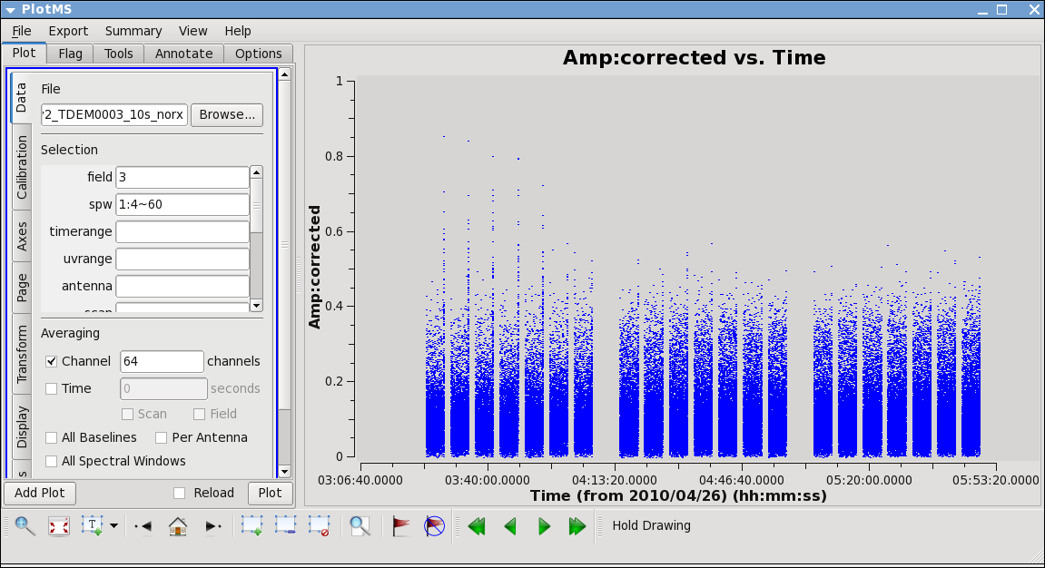
The 95 minutes of on-source time can be estimated from a plot like:
# In CASA
plotms(vis='day2_TDEM0003_10s_norx',field='3',ydatacolumn='corrected',
       xaxis='time',yaxis='amp',correlation='RR,LL',
       avgchannel='64',spw='1:4~60',antenna='')
This analysis suggests that the rms noise on one baseline, one 10 second integration is about 525 mJy. In contrast the peak flux density in the strongest SiS channel is only about 200 mJy (you can check using the viewer). Because the emission is fairly compact, most baselines will see about this peak flux, this is why we chose the more compact of the two possible lines. This peak flux density tells us that we need to use a solint large enough so that the rms noise is not worse than about 1/3 of 200 mJy. Thus, a solint of 10 minutes is about the shortest we can use and be reasonably confident of the solutions.
Now we run gaincal with the solint we have determined. Note that because our desired solint is more than the scan time, we need to include combine='scan'.
# In CASA
gaincal(vis='IRC10216.contsub',caltable='pcal_ch19one_10min',
        spw='1:19~19',calmode='p',solint='10min',combine='scan',
        refant='ea02',minsnr=3.0)
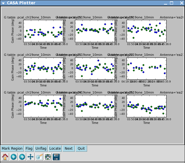
Now let's look at the solutions:
# In CASA
plotcal(caltable='pcal_ch19one_10min',xaxis='time',yaxis='phase',
        iteration='antenna',subplot=331,plotrange=[0,0,-50,50])
For some antennas you can see clear global trends away from zero: ea08, ea21,ea24 are examples, and you can also see some smaller variations with time.
Now let's explore whether applying this solution actually improves matters. To do this we need to run applycal to apply the solutions to the line dataset, both spw. We need to use spwmap to tell it that the solutions derived for spw=1 should be applied to both spw=0 and spw=1. Again it's important to set calwt=F here.
# In CASA
applycal(vis='IRC10216.contsub',field='',spw='0,1',
        gaintable=['pcal_ch19one_10min'],spwmap=[[1,1]],calwt=F)
Note: in this example we ran the self-cal steps on the full uv continuum subtracted spectral line data set. For a more complex iterative self-calibration proceedure, you may find it easier to split off the channel/spw you want to experiment on with split, and then do all the imaging (clean) and gaincal steps with it. The gaincal tables created on the single channel can still be applied with applycal to the multi-channel/spw dataset. If you do this though, keep in mind that once split, the single-channel data will have its spw id reset to 0 (you can check with listobs), no matter what spw it came from. Thus in order to applycal with it you would need spwmap=[[0,0]].
To save time we can use the clean mask we made before and run in a non-interactive mode. You can use a mask over again as long as the number of channels in the clean call haven't changed. You can change cell or imsize and it will still do the right thing.
# In CASA
clean(vis='IRC10216.contsub',imagename='IRC10216_HC3N.cube_r0.5.pselfcal',
      imagermode='csclean',
      imsize=300,cell=['0.4arcsec'],spw='0:5~58',
      mode='velocity',interpolation='linear',
      restfreq='36.39232GHz',outframe='LSRK',
      weighting='briggs',robust=0.5,
      mask='IRC10216_HC3N.cube_r0.5.mask',
      interactive=F,threshold='3.0mJy',niter=100000)
# In CASA
clean(vis='IRC10216.contsub',imagename='IRC10216_SiS.cube_r0.5.pselfcal',
      imagermode='csclean',calready=T,
      imsize=300,cell=['0.4arcsec'],spw='1:5~58',
      mode='velocity',interpolation='linear',
      restfreq='36.30963GHz',outframe='LSRK',
      weighting='briggs',robust=0.5,
      mask='IRC10216_SiS.cube_r0.5.mask',
      interactive=F,threshold='3.0mJy',niter=100000)
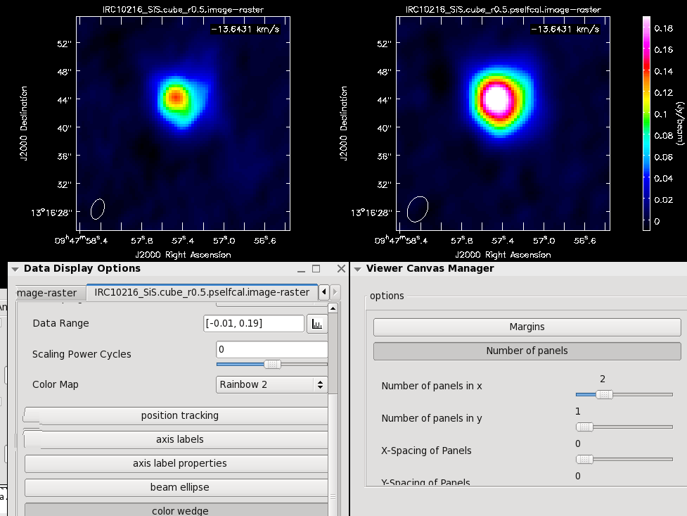
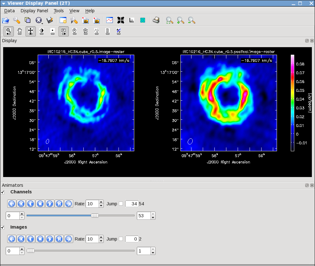
Now investigate the original and self-cal'ed images in the viewer. You will find that even this single self-cal step significantly improves the images. Try opening both versions of the SiS image cubes. Then select a bright channel from the tape deck like channel 37, then use the "wrench" and "pwrench" guis to make a plot like below setting the same image range for both cubes, and two panels in x, then to see both images of that channel side-by-side click the blink toggle (see image below for more tips on setup.)
Repeat for HC3N:
Now you can redo the moment images if you like with the improved cubes, be sure to change the output file names.
Last checked on CASA Version 3.2.0.
