Image Line CASA 6.6.1: Difference between revisions
Created page with "This guide continues from ''' Image the Continuum Template''' and ''' Self-Calibration Template''' (optional). Imaging parameters and calibration tables (if applicable) should already be set prior to continuing. Commands for this guide can be found in scriptForImaging_template.py available on [https://github.com/aakepley/ALMAImagingScript github]. This guide features CARTA, the “Cube Analysis and Rendering Tool for..." |
|||
| (One intermediate revision by the same user not shown) | |||
| Line 30: | Line 30: | ||
This section depends on solutions derived with '''[[Self_Calibration_Template | Self-Calibration Template]]'''. Skip to [[Image_Line#Image_line_emission_.28repeat_as_necessary.29 | Image Line Emission]] if you do not wish to apply self-calibration solutions to the line data. | This section depends on solutions derived with '''[[Self_Calibration_Template | Self-Calibration Template]]'''. Skip to [[Image_Line#Image_line_emission_.28repeat_as_necessary.29 | Image Line Emission]] if you do not wish to apply self-calibration solutions to the line data. | ||
If you find self-calibration does help with lowering the rms in your continuum images, it is a good idea to apply the continuum self-calibration to the line data. Depending on if you performed continuum subtraction, select the definition of linevis accordingly. Once this has been done, it is recommended that you save the flags before you apply the self-calibration solution to the individual line spectral windows, in case you do not like the results or they do not improve the image. If self-calibration of the continuum does improve the quality of the data, apply the derived gaintable to the spectral line channels using the {{applycal_6.6.1}} task. This will improve the image quality of the stronger spectral line channels, but will not help (or harm) the weaker line channels. Then save the results of self-cal in a new ms and reset the image name. You also need to reset the corrected data column in the ms to the original calibration. The | If you find self-calibration does help with lowering the rms in your continuum images, it is a good idea to apply the continuum self-calibration to the line data. Depending on if you performed continuum subtraction, select the definition of linevis accordingly. Once this has been done, it is recommended that you save the flags before you apply the self-calibration solution to the individual line spectral windows, in case you do not like the results or they do not improve the image. If self-calibration of the continuum does improve the quality of the data, apply the derived gaintable to the spectral line channels using the {{applycal_6.6.1}} task. This will improve the image quality of the stronger spectral line channels, but will not help (or harm) the weaker line channels. Then save the results of self-cal in a new ms and reset the image name. You also need to reset the corrected data column in the ms to the original calibration. The {{clearcal_6.6.1}} (linevis) task can also be used to return your ms to its original pre-self-cal state, if you are dissatisfied with the self-calibration results. | ||
<source lang="python"> | <source lang="python"> | ||
# in CASA | # in CASA | ||
| Line 171: | Line 171: | ||
specmode='cube', # comment this if observing an ephemeris source | specmode='cube', # comment this if observing an ephemeris source | ||
# specmode='cubesource', #uncomment this line if observing an ephemeris source | # specmode='cubesource', #uncomment this line if observing an ephemeris source | ||
# perchanweightdensity= | # perchanweightdensity=True #Default setting | ||
start=start, | start=start, | ||
width=width, | width=width, | ||
Revision as of 20:45, 26 November 2024
This guide continues from Image the Continuum Template and Self-Calibration Template (optional). Imaging parameters and calibration tables (if applicable) should already be set prior to continuing. Commands for this guide can be found in scriptForImaging_template.py available on github.
This guide features CARTA, the “Cube Analysis and Rendering Tool for Astronomy,” which is the new NRAO visualization tool for images and cubes. The CASA viewer (imview) has not been maintained for a few years and will be removed from future versions of CASA. We strongly recommend using CARTA, as it provides a much more efficient, stable, and feature rich user experience. A comparison of the CASA viewer and CARTA, as well as instructions on how to use CARTA at NRAO, is provided in the CARTA section of the CASA docs.
Continuum Subtraction for Line Emission
If you have observations that include both line and strong continuum emission (>3 sigma per channel), you should subtract the continuum from the spectral windows before imaging the line. You do not need to continuum subtract if the line of interest is an absorption line.
To subtract the continuum, you need to select channel ranges which only contain continuum. You can use plotms to make sure that the appropriate data is in the appropriate column of your ms. Note that this behavior is different in the pipeline implementation of continuum subtraction hif_uvcontsub. The continuum subtraction routine will then do a linear fit to each integration to determine the continuum and then subtract that linear fit from the data. The range used to fit the continuum is just the opposite of the channels you flagged when creating the continuum (see Create an Averaged Continuum MS section of the Image Continuum guide. You can either manually invert the channels or use the Analysis Utilities routine au.invertChannelRanges to determine the channel ranges. Note that if you use au.invertChannelRanges, you will need to include any continuum spws that weren't in flagchannels. For example, if your continuum spws are '0,1,2' and flagchannels='1:260~500', au.invertChannelRanges will return '1:0~259,1:501~3839'. The fitspw parameter should be '0,1:0~259,1:501~3839,2'. If you haven't installed Analysis Utilities, see Obtaining Analysis Utilities for instructions.
Continuum subtraction is done per field. If all your fields have the same line-free channels, you only have to run uvcontsub once. However, if different fields have different line-free channels, then you will need to run uvcontsub multiple times. (And probably get a cup of coffee or two.)
The output file for uvcontsub will be vis + ".contsub". It will read from the corrected data column if it is present and the data column if the corrected data column is not present.
# in CASA
fitspw = '2:0~1200;1500~3839,3:0~1200;1500~3839' # line free channels. Use au.invertChannelRanges
finalvis='calibrated_final.ms'

uvcontsub(vis=finalvis,
            outputvis=finalvis+'.contsub',
            fitspec=fitspw,  # spw(s) (and channels) to do continuum subtraction on
            fitorder=1,
            intent='OBSERVE_TARGET*')
Apply continuum self-calibration to line data (optional)
This section depends on solutions derived with Self-Calibration Template. Skip to Image Line Emission if you do not wish to apply self-calibration solutions to the line data.
If you find self-calibration does help with lowering the rms in your continuum images, it is a good idea to apply the continuum self-calibration to the line data. Depending on if you performed continuum subtraction, select the definition of linevis accordingly. Once this has been done, it is recommended that you save the flags before you apply the self-calibration solution to the individual line spectral windows, in case you do not like the results or they do not improve the image. If self-calibration of the continuum does improve the quality of the data, apply the derived gaintable to the spectral line channels using the applycal task. This will improve the image quality of the stronger spectral line channels, but will not help (or harm) the weaker line channels. Then save the results of self-cal in a new ms and reset the image name. You also need to reset the corrected data column in the ms to the original calibration. The clearcal (linevis) task can also be used to return your ms to its original pre-self-cal state, if you are dissatisfied with the self-calibration results.
# in CASA
# Uncomment one of the following:
# linevis = finalvis+'.contsub' # if continuum subtracted
# linevis = finalvis  #  if not continuum subtracted
# save original flags in case you don't like the self-cal
flagmanager(vis=linevis,mode='save',versionname='before_selfcal',merge='replace')

spwmap_line = [0] # Mapping self-calibration solution to the individual line spectral windows.
applycal(vis=linevis,
         spwmap=[spwmap_line, spwmap_line], # entering the appropriate spwmap_line value for each spw in the input dataset
         field=field,
         gaintable=['pcal3','apcal'],
         gainfield='',
         calwt=False,
         flagbackup=False,
         interp=['linearperobs','linearperobs'])

# Save results of self-cal in a new ms and reset the image name.
split(vis=linevis,
      outputvis=linevis+'.selfcal',
      datacolumn='corrected')
Image line emission (repeat as necessary)
You should now have a measurement set that is ready to create cubes of the line emission.
If you are new to line imaging, look at First Look at Line Imaging for an introduction to creating line cubes.
You may also find the Automasking Guide useful if you would like tclean to produce the mask for you.
If you expect more complex emission and do not want to create the mask by hand, you can use the directions at Create a Clean Mask from Continuum Image or Moment Cube to create a mask from the dirty cube.
Depending on the observation and the steps you have applied previously, the measurement set may have a variety of names. Make sure to select the correct option below.
# in CASA
finalvis = 'calibrated_final.ms'

# uncomment if you have neither continuum subtracted nor self-calibrated your data
# linevis = finalvis
# uncomment if you have continuum subtracted your data
# linevis = finalvis + '.contsub'
# uncomment if you have both continuum subtracted and self-calibrated your data
# linevis = finalvis + '.contsub.selfcal'
# uncomment if you have only self-calibrated your data
# linevis = finalvis + '.selfcal'
The measurement set indicated in the linevis variable will be used for the rest of the cleaning. Before starting to clean your line cube, run a vishead or listobs to check on the spectral window and field numbers, which may have been re-numbered during the previous steps in the imaging process.
# in CASA
vishead(linevis)
Now you need to set the necessary parameters for tclean. If you haven't already, follow the procedure in the Image Continuum section to set the imsize, cellsize, field, phasecenter,etc. Here we focus on the additional parameters needed to image line data.
First, we set the imagename. Here we name the image for the source and line observed, but you could give it any name you'd like.
# in CASA
sourcename ='n253' # name of source
linename = 'CO10' # name of transition
lineimagename = sourcename+'_'+linename # name of line image
Next select the spws you would like to image. You should only image spws associated with a single rest frequency in the same image. If you have multiple executions and did not regrid the frequency axis using cvel, you will have to select multiple spws (one for each execution). The restfreq is typically set at the rest frequency of the line of interest. If the source is significantly redshifted (z>0.2), common practice is to set the rest frequency to the observed sky frequency (nu_rest/1+z) instead. Then the velocity axis shows offsets from the expected sky frequency.
Finally, if cvel or mstransform was used to regrid spectral windows, make sure to use the same values below as you used with those tasks. In other words, avoid regridding your frequency axis twice: once in cvel and once in tclean.

# in CASA
spw = '0' # update to the spw you would like to image
restfreq='115.27120GHz'
The start, width, and nchan parameters will determine the size of the cube you create. Setting the values at their defaults will image the entire spectral window at the native resolution.
# in CASA
start = ''
width = ''
nchan = -1
You can also image a subset of the cube. By only imaging a subsection of the spectral window you can speed up the time it takes {tclean} to produce a cube and reduces the final size of the cube. This can be done in either velocity space or channel space.
# in CASA
# velocity space
start='-100km/s'
width='2km/s'
nchan = 100

# alternate option
# channel space
start = 1600
width = 1
nchan = 150
Remember that you have already set two specific velocity parameters called outframe and veltype. Outframe is the coordinate system used for the observation. If you have access to the original proposal, this can be found in the Observing Tool (OT) under field setup. A list of acceptable outframes that can be used in CASA can be found at https://help.almascience.org/kb/articles/what-are-the-frequency-reference-frames-in-casa. Note: heliocentric(hel) is deprecated in CASA. Use barycentric(bary) in this case. The most common choices are 'bary' and 'lsrk'. Usually 'bary' is used for 'extragalactic' sources and 'lsrk is used for 'galactic' sources. For ephemeris objects, the outframe should be set to a blank string, for example outframe = '', as the you have likely already regridded to the source velocity.
Generally, if you set outframe = 'bary' and restfreq = observed frequency, the line center should be at around 0 km/s. If you set outframe = 'lsrk' and restfreq = lab frequency, you will need to know the source radial velocity in order to predict the line position. If you are unsure, you can use the plotms command below to plot the visibilities to explore the effects of outframe and restfreq.
You will also have to set the veltype for the tclean command. This variable has only two options available, radio and optical. It is standard to leave this set to ‘radio’ in all projects regardless of the velocity frame used in the project.
# in CASA
outframe='lsrk' # velocity reference frame. See science goals.
veltype='radio' # velocity type.
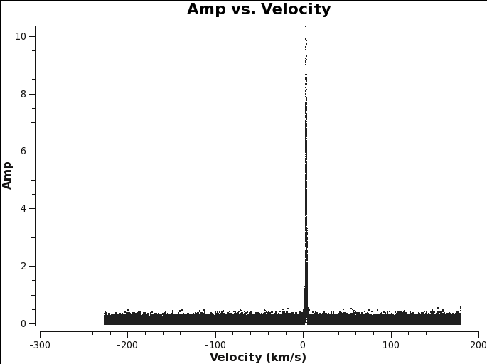
You can use plotms to find the line if it is bright enough to show up in the averaged visibilities. This is similar to the procedure you used to identify the line when creating the averaged continuum ms in Continuum MS.

# in CASA
plotms(vis=linevis,xaxis='velocity',yaxis='amp',avgtime='1e8',avgscan=True,avgantenna=True,
    spw=spw,coloraxis='spw',transform=True,freqframe=outframe.upper(),restfreq=restfreq)
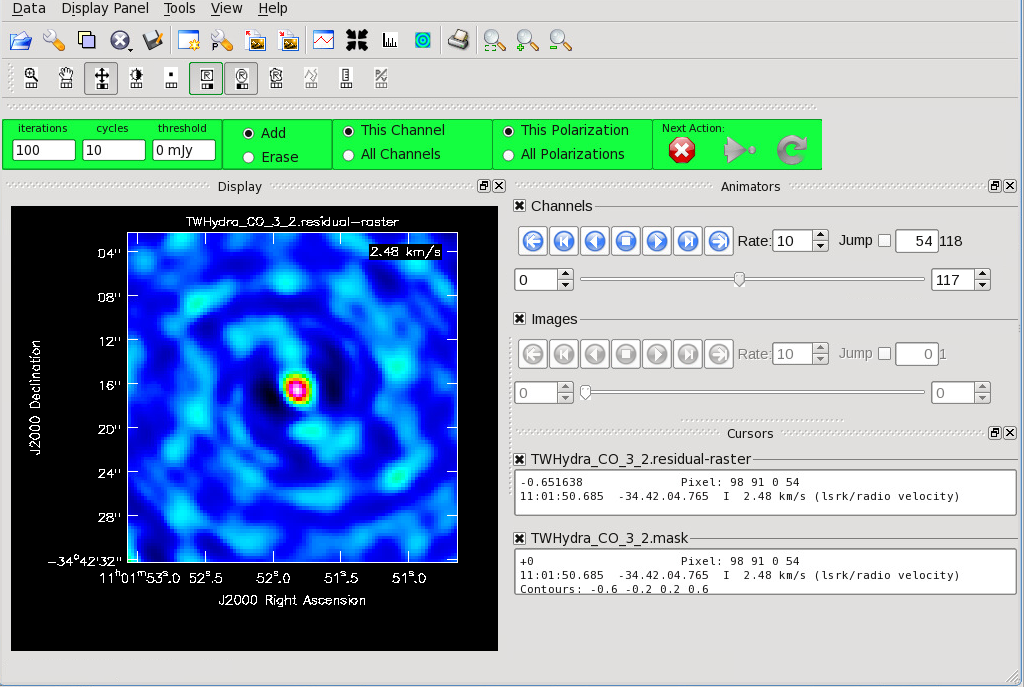
The tclean command for generating your line cube is shown below. You can use this template to image all targeted lines in your observation. For more information about the tclean GUI, see Imaging the Continuum section of the guide.
If you are creating your mask manually, notice that the default is to apply the mask to the current channel you are viewing. The mask can also be applied to all channels. This is indicated with the "This Channel" or "All Channels" toggle.
In CASA 5.4 and later, tclean calls with gridder = 'mosaic' have an additional parameter mosweight with a default of True. When mosweight = True, the gridder weights each field in the mosaic independently. The mosweight parameter is particularly important for mosaics with non-uniform sensitivity, with rectangular shapes, or when using more uniform values of robust Briggs weighting. For more information on mosweight, please see the tclean documentation.
# in CASA
tclean(vis=linevis,
       imagename=lineimagename,
       field=field,
       spw=spw,
       # phasecenter=phasecenter, # uncomment if mosaic or imaging an ephemeris object
       # mosweight=True, # uncomment if mosaic
       specmode='cube', # comment this if observing an ephemeris source
       # specmode='cubesource', #uncomment this line if observing an ephemeris source
       # perchanweightdensity=True #Default setting
       start=start,
       width=width,
       nchan=nchan,
       outframe=outframe,
       veltype=veltype,
       restfreq=restfreq,
       niter=niter,
       threshold=threshold,
       interactive=True,
       cell=cell,
       imsize=imsize,
       weighting=weighting,
       robust=robust,
       gridder=gridder,
       pbcor=True,
       restoringbeam='common',
       usepointing=False)
As you may recall from the continuum imaging section, tclean generates several images with the name imagename+extension every time it cleans an image. If you re-run tclean with the same imagename, tclean will use the existing files as a starting point, continuing the tclean where you left off. To start completely from scratch, either change the imagename or delete all the files from the previous tclean run. Note that CASA retains some image information in memory, so to truly delete the images from open version of CASA, you need to run the rmtables command. See below for an example.
# in CASA
clearcal(vis=linevis)
delmod(vis=linevis)
for ext in ['.image','.mask','.model','.image.pbcor','.psf','.residual','.pb','.sumwt']:
    rmtables(lineimagename + ext)
Export the images
Use exportfits to create fits files of the *.flux and *.pbcor files.
# in CASA
import glob

myimages = glob.glob("*.pbcor")
for image in myimages:
    exportfits(imagename=image, fitsimage=image+'.fits',overwrite=True)

myimages = glob.glob("*.pb")
for image in myimages:
    exportfits(imagename=image, fitsimage=image+'.fits',overwrite=True)
Create Diagnostic PNGs

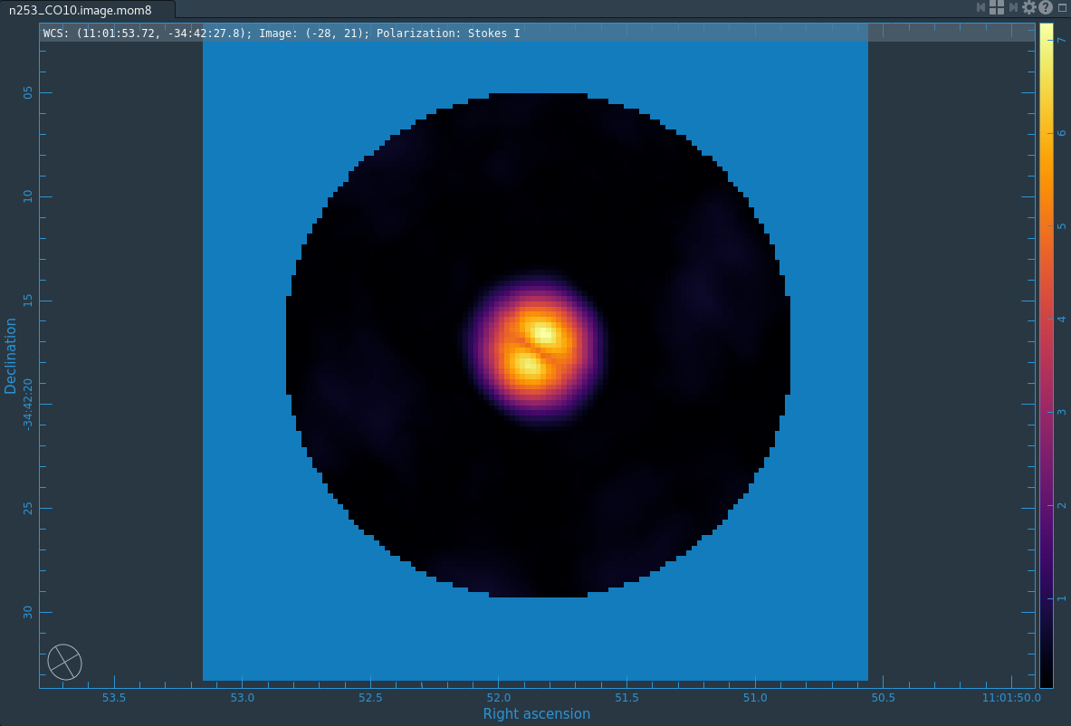
The First Look at Image Analysis guide gives an introduction to a variety of options to begin image analysis, including using immoments to create moment maps. The commands create png files of the continuum image and moment 8 maps, which you can open and examine in CARTA.
# in CASA
os.system("rm -rf *.png")

mylineimages = glob.glob("*cube*manual.image")
for limage in mylineimages:
    mom8=limage+'.mom8'
    os.system("rm -rf "+mom8)
    immoments(limage,moments=[8],outfile=mom8)
    mymax=imstat(mom8)['max'][0]
    mymin=-0.1*mymax
    os.system("rm -rf "+mom8+".png")
    imview(raster={'file':mom8,'range':[mymin,mymax]},out=mom8+'.png')