Sunspot Band6 Calibration for CASA 6.5.4: Difference between revisions
| (11 intermediate revisions by the same user not shown) | |||
| Line 55: | Line 55: | ||
asdm = 'uid___A002_Xae00c5_X2a8d' | asdm = 'uid___A002_Xae00c5_X2a8d' | ||
mso = asdm + '.ms' #MS original | mso = asdm + '.ms' #MS original | ||
mss = asdm + '.ms.split' #MS split | mss = asdm + '.ms.split' #MS split (science spws) | ||
msc = | msc = mss + '.cal' #MS calibrated | ||
</source> | </source> | ||
The raw data have been provided to you in the ASDM format. It is the native format of the data produced by the ALMA observatory. | The raw data have been provided to you in the ASDM format. It is the native format of the data produced by the ALMA observatory. | ||
| Line 66: | Line 66: | ||
</source> | </source> | ||
To fix | To check if a bug fix is needed in the SYSCAL table times, the following commands are executed. | ||
<source lang="python"> | <source lang="python"> | ||
| Line 85: | Line 85: | ||
The output will be sent to the CASA {{logger_6.5.4}}, or saved in a text file. | The output will be sent to the CASA {{logger_6.5.4}}, or saved in a text file. | ||
The first section shows information about the project and observing time: | |||
<pre style="background-color: #fffacd;"> | <pre style="background-color: #fffacd;"> | ||
| Line 96: | Line 96: | ||
====Scan List==== | ====Scan List==== | ||
The second section describes details of each scan. This is often easier to read in a text viewer with line wrapping turned off. We see that our Fields have the following associated intents: | |||
* Field 0 = Sun: observed for the measurement of zero-signal level [scan 1] and the calibration of ''atmosphere'' [scans 10,13,16]. Scientific observations of the Sun ('''Target''') [scans 11,14,17] are listed many times, which represent a mosaic. | |||
* Field 1 = J1924-2914: observed for the calibrations of ''pointing'' [scan 2], ''sideband ratio'' [scan 3], ''atmosphere'' [scan 4], and '''bandpass''' [scan 5] | |||
* Field 2 = nrao530: observed for the calibration of ''pointing'' [scan 6], ''atmosphere'' [scan 7], '''flux''' [scan 8], and '''phase''' [scans 9,12,15,18] | |||
Subscans are NOT necessarily listed in chronological order, but rather ordered by Field ID. For example, for scan 14, Fields 3~9 are observed AFTER Fields 80~150, but listed first. See [[Sunspot_Band6_Imaging_for_CASA_6.5.4#Flag_the_surplus_subscans_and_baselines]]. | |||
<pre style="background-color: #fffacd;"> | <pre style="background-color: #fffacd;"> | ||
| Line 155: | Line 157: | ||
====Field List==== | ====Field List==== | ||
The third section shows the information of the observing targets. This shows that three Sources with 151 Fields were observed: The Sun, J1924-2914, and nrao530 (J1733-1304). The Sun as one Source has many Fields - this is how a mosaic is represented: | |||
<pre style="background-color: #fffacd;"> | <pre style="background-color: #fffacd;"> | ||
| Line 176: | Line 178: | ||
====Spectral Window List==== | ====Spectral Window List==== | ||
The fourth section shows the information of the spws in the dataset. From the scan list, we see that science (Target) scans are done with the spw 0~12. Of these, the spws with 128 channels are 5,7,9,11, which are used for image synthesis. '''Therefore, we will apply calibrations to spws 5,7,9,11 only.''' The data of spws 0,1,2,3 are the data from the square-law detectors of the basebands, which will be used for creating Tsys+Tant tables, and are archived as the auto-correlation data in the dataset. | |||
<pre style="background-color: #fffacd;"> | <pre style="background-color: #fffacd;"> | ||
| Line 220: | Line 222: | ||
</pre> | </pre> | ||
The fifth sections lists the spectral windows (spws) used for each Source. We exclude this for brevity. | |||
====Antenna List==== | ====Antenna List==== | ||
The sixth section shows antenna information. Thirty-one antennas were used for the dataset. Note that numbering in python always begins with "0", so the antennas have IDs 0-30. To see what the antenna configuration looked like at the time of this observation, we use the task {{plotants_6.5.4}} (Figure 1): | |||
<pre style="background-color: #fffacd;"> | <pre style="background-color: #fffacd;"> | ||
| Line 325: | Line 327: | ||
<pre style="background-color: #E0FFFF;"> | <pre style="background-color: #E0FFFF;"> | ||
The Sun is very dynamic, and the time variations of solar structures are one of the main scientific topics of solar physics. To observe such structures, the suspension of science scans are problematic. Therefore, to return to the Sun as quickly as possible, we do NOT perform ATM scans of the phase calibrator in between science scans, instead only observing PHASE intent scans (9,12,15,18). | |||
However, the antenna temperature (Tant) of the Sun is not negligible and must be calibrated. To do this, we perform ATM scans of the blank sky near the Sun, 2 degrees from the Sun's center. Field 0 is used for all calibration scans, and is the center of the mosaic, as we will see later (Fields 3~150 are used for science scans only). The first subscan of science scans (11,14,17) are listed as Field 0, but include the "OBSERVE_TARGET#OFF_SOURCE" intent, which slews to the blank sky. | |||
In this Science Verification observation, one scan of the phase calibrator has ATM intent (scan 7) before any science scans begin, but more recent solar observations do not include this. Scan 7 can be ignored. | |||
</pre> | </pre> | ||
'''For details, see [https://arxiv.org/abs/1704.03236v2 Shimojo+ 2017], in particular Figure 4.''' | |||
Therefore, we calibrate the Tsys of the phase calibrator ''(field='2')'' by applying the calibrations for the Sun ''(gainfield='0')'', as follows: | Therefore, we calibrate the Tsys of the phase calibrator ''(field='2')'' by applying the calibrations for the Sun ''(gainfield='0')'', as follows: | ||
| Line 426: | Line 430: | ||
Now {{split_6.5.4}} out the CORRECTED data column, retaining spectral windows 5,7,9,11. This will get rid of the extraneous spectral windows. | Now {{split_6.5.4}} out the CORRECTED data column, retaining spectral windows 5,7,9,11. This will get rid of the extraneous spectral windows. | ||
<source lang="python"> | <source lang="python"> | ||
#In CASA | #In CASA | ||
split(vis=mso, outputvis=mss, datacolumn='corrected', intent ='*BANDPASS*,*FLUX*,*PHASE*,*TARGET*', spw='5,7,9,11' | split(vis=mso, outputvis=mss, datacolumn='corrected', intent ='*BANDPASS*,*FLUX*,*PHASE*,*TARGET*', spw='5,7,9,11') | ||
</source> | </source> | ||
| Line 593: | Line 596: | ||
[[Image:sunspot_flux_inf.png|300px|thumb|right|'''Fig. 7.''' Example of the flux-scaled amplitude calibration table.]] | [[Image:sunspot_flux_inf.png|300px|thumb|right|'''Fig. 7.''' Example of the flux-scaled amplitude calibration table.]] | ||
<source lang='python'> | <source lang='python'> | ||
| Line 650: | Line 652: | ||
<source lang='python'> | <source lang='python'> | ||
#In CASA | #In CASA | ||
applycal(vis=mss, field='0, 3~150', gaintable=[mss+'.bandpass', mss+'.phase_inf', mss+'.flux_inf'], gainfield=['', '2', ''], | applycal(vis=mss, field='0, 3~150', gaintable=[mss+'.bandpass', mss+'.phase_inf', mss+'.flux_inf'], gainfield=['', '2', '2'], | ||
interp='linear,linear', calwt=True, flagbackup=False) | interp='linear,linear', calwt=True, flagbackup=False) | ||
</source> | </source> | ||
| Line 658: | Line 660: | ||
<source lang='python'> | <source lang='python'> | ||
#In CASA | #In CASA | ||
split(vis=mss, outputvis=msc, datacolumn='corrected' | split(vis=mss, outputvis=msc, datacolumn='corrected') | ||
</source> | </source> | ||
==Re-calculation of the direction== | ==Re-calculation of the direction== | ||
[[File: | [[File:sunspot_mos1.png|thumb|right|'''Fig. 3.''' The pattern of mosaic BEFORE the re-calculation of the direction.]] | ||
[[File:sunspot_mosaic_after_CASA_6.5.4.png|thumb|right|'''Fig. 4.''' The pattern of mosaic AFTER the re-calculation of the direction.]] | [[File:sunspot_mosaic_after_CASA_6.5.4.png|thumb|right|'''Fig. 4.''' The pattern of mosaic AFTER the re-calculation of the direction.]] | ||
During most solar observations, the antennas are tracking a structure on the Sun according to the solar differential rotation. The image frame is fixed on the solar frame, but the frame is moving on the RA/Dec coordinate frame. If we do not | During most solar observations, the antennas are tracking a structure on the Sun according to the solar differential rotation. The image frame is fixed on the solar frame, but the frame is moving on the RA/Dec coordinate frame. If we do not correct for this, the pattern of pointing in the mosaic is a rhombus as shown in Figure 3, while the correct shape should be a square. | ||
Plot the mosaic to see this: | Plot the mosaic to see this:<br> | ||
<font color="red"> | |||
The following command does not correctly create the plot as shown in Figure 3 at this time. Figure 3 is taken from a previous version of this guide. | |||
</font> | |||
<source lang='python'> | <source lang='python'> | ||
| Line 680: | Line 685: | ||
#In CASA | #In CASA | ||
reftime = '2015/12/18/19:49:00' | reftime = '2015/12/18/19:49:00' | ||
fixplanets(msc, field='0', fixuvw=False, refant=ref_ant, reftime=reftime) | fixplanets(vis=msc, field='0', fixuvw=False, refant=ref_ant, reftime=reftime) | ||
</source> | </source> | ||
| Line 700: | Line 705: | ||
offRaDec = aU.radec2deg(aU.radecOffsetToRadec(refRaDec, raOff, deOff, prec=1)) | offRaDec = aU.radec2deg(aU.radecOffsetToRadec(refRaDec, raOff, deOff, prec=1)) | ||
offRaDecF = 'J2000 ' + aU.deg2radec(offRaDec[0], offRaDec[1], prec=1, hmsdms=True, delimiter=' ') | offRaDecF = 'J2000 ' + aU.deg2radec(offRaDec[0], offRaDec[1], prec=1, hmsdms=True, delimiter=' ') | ||
fixplanets(msc, field=str(i), fixuvw=False, direction=offRaDecF) | fixplanets(vis=msc, field=str(i), fixuvw=False, direction=offRaDecF) | ||
tb.open(msc+'/FIELD', nomodify=False) | tb.open(msc+'/FIELD', nomodify=False) | ||
Latest revision as of 16:35, 22 April 2024
Last checked on CASA Version 6.5.4
Getting Started
Details of these ALMA observations are provided at Sunspot_Band6. This portion of the guide will cover the calibration of the raw visibility data.
WARNING: The command in the #Tsys+Tant calibration of the Sun section of this guide takes a long time to run. Depending on your machine, it may be between a couple hours and one day.
Download and Unpack the Data
To follow this guide you must download the file Sunspot_Band6_UncalibratedData.tgz from Sunspot_Band6#Obtaining the Data.
Unpack and cd to the directory:
#In bash
tar -xvzf Sunspot_Band6_UncalibratedData.tgz
cd Sunspot_Band6_UncalibratedData
Confirm your version of CASA
This guide has been written for CASA release 6.5. Start CASA and confirm your version before proceeding.
# In CASA
from casatools import version
vernum = str(version()[0])+'.'+str(version()[1])
print("You are using CASA ver. "+vernum)
if float(vernum) < 6.5:
 print("YOUR VERSION OF CASA IS TOO OLD FOR THIS GUIDE.")
 print("PLEASE UPDATE IT BEFORE PROCEEDING.")
else:
 print("Your version of CASA is appropriate for this guide.")
Import Tools and Scripts
The "Analysis Utilities" package must be used for the calibration of raw solar visibility data. Therefore, before starting the tutorial, you need to import the package to your data-analysis environment. The documents and software of the package can be obtained from the Analysis_Utilities guide.
We also need script to download the script Sun_reduction_util_6.5.4.py and execute it inside our CASA session.
#In CASA
import analysisUtils as aU
es = aU.stuffForScienceDataReduction()
execfile('Sun_reduction_util_6.5.4.py')
Initial Inspection
Import the Data into CASA
We start by defining the directory name of the ASDM and some directory names of the Measurement Sets (MS) for the calibration.
#In CASA
asdm = 'uid___A002_Xae00c5_X2a8d'
mso = asdm + '.ms'           #MS original
mss = asdm + '.ms.split'     #MS split (science spws)
msc = mss  + '.cal'          #MS calibrated
The raw data have been provided to you in the ASDM format. It is the native format of the data produced by the ALMA observatory.
Before we can proceed to the calibration, we will need to convert those data to the CASA MS format. This is done simply with the task importasdm.
#In CASA
importasdm(asdm=asdm, vis=mso, asis='Antenna Station Receiver Source CalAtmosphere CalWVR CorrelatorMode SBSummary CalDevice')
To check if a bug fix is needed in the SYSCAL table times, the following commands are executed.
#In CASA
from casarecipes.almahelpers import fixsyscaltimes
fixsyscaltimes(vis=mso)
Inspect the Data
The usual first step is then to get some basic information about the data. We do this using the task listobs, which will output a detailed summary of each dataset supplied.
#In CASA
listobs(mso, listfile=asdm+'.listobs.txt')
The output will be sent to the CASA logger, or saved in a text file.
The first section shows information about the project and observing time:
   Observer: shimojo     Project: uid://A002/Xac494e/X3
Observation: ALMA
Data records: 20923884       Total elapsed time = 3184.8 seconds
   Observed from   18-Dec-2015/19:15:42.3   to   18-Dec-2015/20:08:47.1 (UTC)
Scan List
The second section describes details of each scan. This is often easier to read in a text viewer with line wrapping turned off. We see that our Fields have the following associated intents:
- Field 0 = Sun: observed for the measurement of zero-signal level [scan 1] and the calibration of atmosphere [scans 10,13,16]. Scientific observations of the Sun (Target) [scans 11,14,17] are listed many times, which represent a mosaic.
- Field 1 = J1924-2914: observed for the calibrations of pointing [scan 2], sideband ratio [scan 3], atmosphere [scan 4], and bandpass [scan 5]
- Field 2 = nrao530: observed for the calibration of pointing [scan 6], atmosphere [scan 7], flux [scan 8], and phase [scans 9,12,15,18]
Subscans are NOT necessarily listed in chronological order, but rather ordered by Field ID. For example, for scan 14, Fields 3~9 are observed AFTER Fields 80~150, but listed first. See Sunspot_Band6_Imaging_for_CASA_6.5.4#Flag_the_surplus_subscans_and_baselines.
   ObservationID = 0         ArrayID = 0
  Date        Timerange (UTC)          Scan  FldId FieldName             nRows     SpwIds   Average Interval(s)    ScanIntent
  18-Dec-2015/19:15:42.3 - 19:16:47.5     1      0 Sun                     236530  [0,1,2,3,4,5,6,7,8,9,10,11,12,13,14,15,16,17,18,19,20,21,22,23,24]  [0.016, 0.016, 0.016, 0.016, 1.15, 0.576, 0.576, 0.576, 0.576, 0.576, 0.576, 0.576, 0.576, 0.016, 0.016, 0.016, 0.016, 0.576, 0.576, 0.576, 0.576, 0.576, 0.576, 0.576, 0.576] [CALIBRATE_ATMOSPHERE#AMBIENT,CALIBRATE_ATMOSPHERE#HOT,CALIBRATE_ATMOSPHERE#OFF_SOURCE,CALIBRATE_ATMOSPHERE#REFERENCE,CALIBRATE_WVR#AMBIENT,CALIBRATE_WVR#HOT,CALIBRATE_WVR#OFF_SOURCE,CALIBRATE_WVR#REFERENCE]
              19:17:31.8 - 19:19:26.4     2      1 J1924-2914             1081497  [4,25,26,27,28,29,30,31,32,33,34,35,36]  [1.15, 0.016, 0.016, 0.016, 0.016, 2.02, 1.01, 2.02, 1.01, 2.02, 1.01, 2.02, 1.01] [CALIBRATE_POINTING#ON_SOURCE,CALIBRATE_WVR#ON_SOURCE]
              19:20:14.2 - 19:21:17.7     3      1 J1924-2914              895435  [0,1,2,3,4,5,6,7,8,9,10,11,12]  [0.016, 0.016, 0.016, 0.016, 1.15, 0.576, 0.576, 0.576, 0.576, 0.576, 0.576, 0.576, 0.576] [CALIBRATE_SIDEBAND_RATIO#IMAGE,CALIBRATE_SIDEBAND_RATIO#SIGNAL,CALIBRATE_WVR#IMAGE,CALIBRATE_WVR#SIGNAL]
              19:22:06.0 - 19:22:23.1     4      1 J1924-2914              177382  [0,1,2,3,4,5,6,7,8,9,10,11,12]  [0.016, 0.016, 0.016, 0.016, 1.15, 0.576, 0.576, 0.576, 0.576, 0.576, 0.576, 0.576, 0.576] [CALIBRATE_ATMOSPHERE#AMBIENT,CALIBRATE_ATMOSPHERE#HOT,CALIBRATE_ATMOSPHERE#OFF_SOURCE,CALIBRATE_WVR#AMBIENT,CALIBRATE_WVR#HOT,CALIBRATE_WVR#OFF_SOURCE]
              19:23:11.6 - 19:28:27.9     5      1 J1924-2914             3244522  [0,1,2,3,4,5,6,7,8,9,10,11,12]  [0.016, 0.016, 0.016, 0.016, 1.15, 2.02, 1.01, 2.02, 1.01, 2.02, 1.01, 2.02, 1.01] [CALIBRATE_BANDPASS#ON_SOURCE,CALIBRATE_WVR#ON_SOURCE]
              19:29:14.5 - 19:31:09.2     6      2 nrao530                1081528  [4,25,26,27,28,29,30,31,32,33,34,35,36]  [1.15, 0.016, 0.016, 0.016, 0.016, 2.02, 1.01, 2.02, 1.01, 2.02, 1.01, 2.02, 1.01] [CALIBRATE_POINTING#ON_SOURCE,CALIBRATE_WVR#ON_SOURCE]
              19:31:54.6 - 19:32:11.4     7      2 nrao530                 177413  [0,1,2,3,4,5,6,7,8,9,10,11,12]  [0.016, 0.016, 0.016, 0.016, 1.15, 0.576, 0.576, 0.576, 0.576, 0.576, 0.576, 0.576, 0.576] [CALIBRATE_ATMOSPHERE#AMBIENT,CALIBRATE_ATMOSPHERE#HOT,CALIBRATE_ATMOSPHERE#OFF_SOURCE,CALIBRATE_WVR#AMBIENT,CALIBRATE_WVR#HOT,CALIBRATE_WVR#OFF_SOURCE]
              19:32:59.1 - 19:35:36.6     8      2 nrao530                1622261  [0,1,2,3,4,5,6,7,8,9,10,11,12]  [0.016, 0.016, 0.016, 0.016, 1.15, 2.02, 1.01, 2.02, 1.01, 2.02, 1.01, 2.02, 1.01] [CALIBRATE_FLUX#ON_SOURCE,CALIBRATE_WVR#ON_SOURCE]
              19:36:21.9 - 19:36:52.1     9      2 nrao530                 324446  [0,1,2,3,4,5,6,7,8,9,10,11,12]  [0.016, 0.016, 0.016, 0.016, 1.15, 2.02, 1.01, 2.02, 1.01, 2.02, 1.01, 2.02, 1.01] [CALIBRATE_PHASE#ON_SOURCE,CALIBRATE_WVR#ON_SOURCE]
              19:37:41.4 - 19:37:57.8    10      0 Sun                     177413  [0,1,2,3,4,5,6,7,8,9,10,11,12]  [0.016, 0.016, 0.016, 0.016, 1.15, 0.576, 0.576, 0.576, 0.576, 0.576, 0.576, 0.576, 0.576] [CALIBRATE_ATMOSPHERE#AMBIENT,CALIBRATE_ATMOSPHERE#HOT,CALIBRATE_ATMOSPHERE#OFF_SOURCE,CALIBRATE_WVR#AMBIENT,CALIBRATE_WVR#HOT,CALIBRATE_WVR#OFF_SOURCE]
              19:39:23.9 - 19:49:36.0    11      0 Sun                    3760610  [0,1,2,3,4,5,6,7,8,9,10,11,12]  [0.016, 0.016, 0.016, 0.016, 1.15, 2.02, 1.01, 2.02, 1.01, 2.02, 1.01, 2.02, 1.01] [CALIBRATE_WVR#OFF_SOURCE,CALIBRATE_WVR#ON_SOURCE,OBSERVE_TARGET#OFF_SOURCE,OBSERVE_TARGET#ON_SOURCE]
              19:39:23.9 - 19:49:36.0    11      3 Sun                      18011  [4,5,6,7,8,9,10,11,12]  [1.15, 2.02, 1.01, 2.02, 1.01, 2.02, 1.01, 2.02, 1.01] [CALIBRATE_WVR#ON_SOURCE,OBSERVE_TARGET#ON_SOURCE]
              19:39:23.9 - 19:49:36.0    11      4 Sun                      18011  [4,5,6,7,8,9,10,11,12]  [1.15, 2.02, 1.01, 2.02, 1.01, 2.02, 1.01, 2.02, 1.01] [CALIBRATE_WVR#ON_SOURCE,OBSERVE_TARGET#ON_SOURCE]
              19:39:23.9 - 19:49:36.0    11      5 Sun                      18042  [4,5,6,7,8,9,10,11,12]  [1.15, 2.02, 1.01, 2.02, 1.01, 2.02, 1.01, 2.02, 1.01] [CALIBRATE_WVR#ON_SOURCE,OBSERVE_TARGET#ON_SOURCE]

*** Scan 11, Fields 6~76 trimmed for brevity ***

              19:39:23.9 - 19:49:36.0    11     77 Sun                      18011  [4,5,6,7,8,9,10,11,12]  [1.15, 2.02, 1.01, 2.02, 1.01, 2.02, 1.01, 2.02, 1.01] [CALIBRATE_WVR#ON_SOURCE,OBSERVE_TARGET#ON_SOURCE]
              19:39:23.9 - 19:49:36.0    11     78 Sun                      18042  [4,5,6,7,8,9,10,11,12]  [1.15, 2.02, 1.01, 2.02, 1.01, 2.02, 1.01, 2.02, 1.01] [CALIBRATE_WVR#ON_SOURCE,OBSERVE_TARGET#ON_SOURCE]
              19:39:23.9 - 19:49:36.0    11     79 Sun                      18011  [4,5,6,7,8,9,10,11,12]  [1.15, 2.02, 1.01, 2.02, 1.01, 2.02, 1.01, 2.02, 1.01] [CALIBRATE_WVR#ON_SOURCE,OBSERVE_TARGET#ON_SOURCE]
              19:50:21.7 - 19:50:52.0    12      2 nrao530                 324446  [0,1,2,3,4,5,6,7,8,9,10,11,12]  [0.016, 0.016, 0.016, 0.016, 1.15, 2.02, 1.01, 2.02, 1.01, 2.02, 1.01, 2.02, 1.01] [CALIBRATE_PHASE#ON_SOURCE,CALIBRATE_WVR#ON_SOURCE]
              19:51:41.2 - 19:51:58.0    13      0 Sun                     177413  [0,1,2,3,4,5,6,7,8,9,10,11,12]  [0.016, 0.016, 0.016, 0.016, 1.15, 0.576, 0.576, 0.576, 0.576, 0.576, 0.576, 0.576, 0.576] [CALIBRATE_ATMOSPHERE#AMBIENT,CALIBRATE_ATMOSPHERE#HOT,CALIBRATE_ATMOSPHERE#OFF_SOURCE,CALIBRATE_WVR#AMBIENT,CALIBRATE_WVR#HOT,CALIBRATE_WVR#OFF_SOURCE]
              19:53:26.0 - 20:03:37.0    14      0 Sun                    3742537  [0,1,2,3,4,5,6,7,8,9,10,11,12]  [0.016, 0.016, 0.016, 0.016, 1.15, 2.02, 1.01, 2.02, 1.01, 2.02, 1.01, 2.02, 1.01] [CALIBRATE_WVR#OFF_SOURCE,CALIBRATE_WVR#ON_SOURCE,OBSERVE_TARGET#OFF_SOURCE,OBSERVE_TARGET#ON_SOURCE]
              19:53:26.0 - 20:03:37.0    14      3 Sun                      18011  [4,5,6,7,8,9,10,11,12]  [1.15, 2.02, 1.01, 2.02, 1.01, 2.02, 1.01, 2.02, 1.01] [CALIBRATE_WVR#ON_SOURCE,OBSERVE_TARGET#ON_SOURCE]
              19:53:26.0 - 20:03:37.0    14      4 Sun                      18042  [4,5,6,7,8,9,10,11,12]  [1.15, 2.02, 1.01, 2.02, 1.01, 2.02, 1.01, 2.02, 1.01] [CALIBRATE_WVR#ON_SOURCE,OBSERVE_TARGET#ON_SOURCE]
              19:53:26.0 - 20:03:37.0    14      5 Sun                      18011  [4,5,6,7,8,9,10,11,12]  [1.15, 2.02, 1.01, 2.02, 1.01, 2.02, 1.01, 2.02, 1.01] [CALIBRATE_WVR#ON_SOURCE,OBSERVE_TARGET#ON_SOURCE]
              19:53:26.0 - 20:03:37.0    14      6 Sun                      18042  [4,5,6,7,8,9,10,11,12]  [1.15, 2.02, 1.01, 2.02, 1.01, 2.02, 1.01, 2.02, 1.01] [CALIBRATE_WVR#ON_SOURCE,OBSERVE_TARGET#ON_SOURCE]
              19:53:26.0 - 20:03:37.0    14      7 Sun                      18011  [4,5,6,7,8,9,10,11,12]  [1.15, 2.02, 1.01, 2.02, 1.01, 2.02, 1.01, 2.02, 1.01] [CALIBRATE_WVR#ON_SOURCE,OBSERVE_TARGET#ON_SOURCE]
              19:53:26.0 - 20:03:37.0    14      8 Sun                      18011  [4,5,6,7,8,9,10,11,12]  [1.15, 2.02, 1.01, 2.02, 1.01, 2.02, 1.01, 2.02, 1.01] [CALIBRATE_WVR#ON_SOURCE,OBSERVE_TARGET#ON_SOURCE]
              19:53:26.0 - 20:03:37.0    14      9 Sun                      18011  [4,5,6,7,8,9,10,11,12]  [1.15, 2.02, 1.01, 2.02, 1.01, 2.02, 1.01, 2.02, 1.01] [CALIBRATE_WVR#ON_SOURCE,OBSERVE_TARGET#ON_SOURCE]
              19:53:26.0 - 20:03:37.0    14     80 Sun                      18042  [4,5,6,7,8,9,10,11,12]  [1.15, 2.02, 1.01, 2.02, 1.01, 2.02, 1.01, 2.02, 1.01] [CALIBRATE_WVR#ON_SOURCE,OBSERVE_TARGET#ON_SOURCE]
              19:53:26.0 - 20:03:37.0    14     81 Sun                      18011  [4,5,6,7,8,9,10,11,12]  [1.15, 2.02, 1.01, 2.02, 1.01, 2.02, 1.01, 2.02, 1.01] [CALIBRATE_WVR#ON_SOURCE,OBSERVE_TARGET#ON_SOURCE]
              19:53:26.0 - 20:03:37.0    14     82 Sun                      18042  [4,5,6,7,8,9,10,11,12]  [1.15, 2.02, 1.01, 2.02, 1.01, 2.02, 1.01, 2.02, 1.01] [CALIBRATE_WVR#ON_SOURCE,OBSERVE_TARGET#ON_SOURCE]

*** Scan 14, Fields 83~147 trimmed for brevity ***

              19:53:26.0 - 20:03:37.0    14    148 Sun                      18011  [4,5,6,7,8,9,10,11,12]  [1.15, 2.02, 1.01, 2.02, 1.01, 2.02, 1.01, 2.02, 1.01] [CALIBRATE_WVR#ON_SOURCE,OBSERVE_TARGET#ON_SOURCE]
              19:53:26.0 - 20:03:37.0    14    149 Sun                      18011  [4,5,6,7,8,9,10,11,12]  [1.15, 2.02, 1.01, 2.02, 1.01, 2.02, 1.01, 2.02, 1.01] [CALIBRATE_WVR#ON_SOURCE,OBSERVE_TARGET#ON_SOURCE]
              19:53:26.0 - 20:03:37.0    14    150 Sun                      18011  [4,5,6,7,8,9,10,11,12]  [1.15, 2.02, 1.01, 2.02, 1.01, 2.02, 1.01, 2.02, 1.01] [CALIBRATE_WVR#ON_SOURCE,OBSERVE_TARGET#ON_SOURCE]
              20:04:22.7 - 20:04:53.7    15      2 nrao530                 324446  [0,1,2,3,4,5,6,7,8,9,10,11,12]  [0.016, 0.016, 0.016, 0.016, 1.15, 2.02, 1.01, 2.02, 1.01, 2.02, 1.01, 2.02, 1.01] [CALIBRATE_PHASE#ON_SOURCE,CALIBRATE_WVR#ON_SOURCE]
              20:05:43.3 - 20:06:00.2    16      0 Sun                     177413  [0,1,2,3,4,5,6,7,8,9,10,11,12]  [0.016, 0.016, 0.016, 0.016, 1.15, 0.576, 0.576, 0.576, 0.576, 0.576, 0.576, 0.576, 0.576] [CALIBRATE_ATMOSPHERE#AMBIENT,CALIBRATE_ATMOSPHERE#HOT,CALIBRATE_ATMOSPHERE#OFF_SOURCE,CALIBRATE_WVR#AMBIENT,CALIBRATE_WVR#HOT,CALIBRATE_WVR#OFF_SOURCE]
              20:06:47.8 - 20:07:30.5    17      0 Sun                     227168  [0,1,2,3,4,5,6,7,8,9,10,11,12]  [0.016, 0.016, 0.016, 0.016, 1.15, 2.02, 1.01, 2.02, 1.01, 2.02, 1.01, 2.02, 1.01] [CALIBRATE_WVR#OFF_SOURCE,CALIBRATE_WVR#ON_SOURCE,OBSERVE_TARGET#OFF_SOURCE,OBSERVE_TARGET#ON_SOURCE]
              20:06:47.8 - 20:07:30.5    17     10 Sun                      18011  [4,5,6,7,8,9,10,11,12]  [1.15, 2.02, 1.01, 2.02, 1.01, 2.02, 1.01, 2.02, 1.01] [CALIBRATE_WVR#ON_SOURCE,OBSERVE_TARGET#ON_SOURCE]
              20:06:47.8 - 20:07:30.5    17     11 Sun                      18042  [4,5,6,7,8,9,10,11,12]  [1.15, 2.02, 1.01, 2.02, 1.01, 2.02, 1.01, 2.02, 1.01] [CALIBRATE_WVR#ON_SOURCE,OBSERVE_TARGET#ON_SOURCE]
              20:06:47.8 - 20:07:30.5    17     12 Sun                      18011  [4,5,6,7,8,9,10,11,12]  [1.15, 2.02, 1.01, 2.02, 1.01, 2.02, 1.01, 2.02, 1.01] [CALIBRATE_WVR#ON_SOURCE,OBSERVE_TARGET#ON_SOURCE]
              20:08:16.5 - 20:08:47.1    18      2 nrao530                 324446  [0,1,2,3,4,5,6,7,8,9,10,11,12]  [0.016, 0.016, 0.016, 0.016, 1.15, 2.02, 1.01, 2.02, 1.01, 2.02, 1.01, 2.02, 1.01] [CALIBRATE_PHASE#ON_SOURCE,CALIBRATE_WVR#ON_SOURCE]
           (nRows = Total number of rows per scan)
Field List
The third section shows the information of the observing targets. This shows that three Sources with 151 Fields were observed: The Sun, J1924-2914, and nrao530 (J1733-1304). The Sun as one Source has many Fields - this is how a mosaic is represented:
Fields: 151
  ID   Code Name                RA               Decl           Epoch   SrcId      nRows
  0    none Sun                 17:44:04.359217 -23.19.29.92535 ICRS    0        8499084
  1    none J1924-2914          19:24:51.055957 -29.14.30.12103 ICRS    1        5398836
  2    none nrao530             17:33:02.705760 -13.04.49.54800 ICRS    2        4178986
  3    none Sun                 17:44:03.784899 -23.20.37.96258 ICRS    0          36022
  4    none Sun                 17:44:04.746002 -23.20.37.96880 ICRS    0          36053
  5    none Sun                 17:44:05.707104 -23.20.37.97466 ICRS    0          36053

*** Sun Fields 6~147 trimmed for brevity ***

  148  none Sun                 17:44:15.209549 -23.18.24.35893 ICRS    0          18011
  149  none Sun                 17:44:16.170347 -23.18.24.36194 ICRS    0          18011
  150  none Sun                 17:44:17.131145 -23.18.24.36460 ICRS    0          18011
Spectral Window List
The fourth section shows the information of the spws in the dataset. From the scan list, we see that science (Target) scans are done with the spw 0~12. Of these, the spws with 128 channels are 5,7,9,11, which are used for image synthesis. Therefore, we will apply calibrations to spws 5,7,9,11 only. The data of spws 0,1,2,3 are the data from the square-law detectors of the basebands, which will be used for creating Tsys+Tant tables, and are archived as the auto-correlation data in the dataset.
Spectral Windows:  (37 unique spectral windows and 2 unique polarization setups)
  SpwID  Name                                       #Chans   Frame   Ch0(MHz)  ChanWid(kHz)  TotBW(kHz) CtrFreq(MHz) BBC Num  Corrs
  0      BB_1#SQLD                                       1   TOPO  230000.000   2000000.000   2000000.0 230000.0000        1  XX  YY
  1      BB_2#SQLD                                       1   TOPO  232000.000   2000000.000   2000000.0 232000.0000        2  XX  YY
  2      BB_3#SQLD                                       1   TOPO  246000.000   2000000.000   2000000.0 246000.0000        3  XX  YY
  3      BB_4#SQLD                                       1   TOPO  248000.000   2000000.000   2000000.0 248000.0000        4  XX  YY
  4      WVR#NOMINAL                                     4   TOPO  184550.000   1500000.000   7500000.0 187550.0000        0  XX
  5      X241538345#ALMA_RB_06#BB_1#SW-01#FULL_RES     128   TOPO  230992.188    -15625.000   2000000.0 230000.0000        1  XX  YY
  6      X241538345#ALMA_RB_06#BB_1#SW-01#CH_AVG         1   TOPO  229984.375   1796875.000   1796875.0 229984.3750        1  XX  YY
  7      X241538345#ALMA_RB_06#BB_2#SW-01#FULL_RES     128   TOPO  232992.188    -15625.000   2000000.0 232000.0000        2  XX  YY
  8      X241538345#ALMA_RB_06#BB_2#SW-01#CH_AVG         1   TOPO  231984.375   1796875.000   1796875.0 231984.3750        2  XX  YY
  9      X241538345#ALMA_RB_06#BB_3#SW-01#FULL_RES     128   TOPO  245007.813     15625.000   2000000.0 246000.0000        3  XX  YY
  10     X241538345#ALMA_RB_06#BB_3#SW-01#CH_AVG         1   TOPO  245984.375   1796875.000   1796875.0 245984.3750        3  XX  YY
  11     X241538345#ALMA_RB_06#BB_4#SW-01#FULL_RES     128   TOPO  247007.813     15625.000   2000000.0 248000.0000        4  XX  YY
  12     X241538345#ALMA_RB_06#BB_4#SW-01#CH_AVG         1   TOPO  247984.375   1796875.000   1796875.0 247984.3750        4  XX  YY
  13     BB_1#SQLD                                       1   TOPO  219559.000   2000000.000   2000000.0 219559.0000        1  XX  YY
  14     BB_2#SQLD                                       1   TOPO  219559.000   2000000.000   2000000.0 219559.0000        2  XX  YY
  15     BB_3#SQLD                                       1   TOPO  219559.000   2000000.000   2000000.0 219559.0000        3  XX  YY
  16     BB_4#SQLD                                       1   TOPO  219559.000   2000000.000   2000000.0 219559.0000        4  XX  YY
  17     X241538345#ALMA_RB_06#BB_1#SW-01#FULL_RES     128   TOPO  220551.188    -15625.000   2000000.0 219559.0000        1  XX  YY
  18     X241538345#ALMA_RB_06#BB_1#SW-01#CH_AVG         1   TOPO  219543.375   1796875.000   1796875.0 219543.3750        1  XX  YY
  19     X241538345#ALMA_RB_06#BB_2#SW-01#FULL_RES     128   TOPO  220551.188    -15625.000   2000000.0 219559.0000        2  XX  YY
  20     X241538345#ALMA_RB_06#BB_2#SW-01#CH_AVG         1   TOPO  219543.375   1796875.000   1796875.0 219543.3750        2  XX  YY
  21     X241538345#ALMA_RB_06#BB_3#SW-01#FULL_RES     128   TOPO  220551.188    -15625.000   2000000.0 219559.0000        3  XX  YY
  22     X241538345#ALMA_RB_06#BB_3#SW-01#CH_AVG         1   TOPO  219543.375   1796875.000   1796875.0 219543.3750        3  XX  YY
  23     X241538345#ALMA_RB_06#BB_4#SW-01#FULL_RES     128   TOPO  220551.188    -15625.000   2000000.0 219559.0000        4  XX  YY
  24     X241538345#ALMA_RB_06#BB_4#SW-01#CH_AVG         1   TOPO  219543.375   1796875.000   1796875.0 219543.3750        4  XX  YY
  25     BB_1#SQLD                                       1   TOPO  221538.000   2000000.000   2000000.0 221538.0000        1  XX  YY
  26     BB_2#SQLD                                       1   TOPO  223538.000   2000000.000   2000000.0 223538.0000        2  XX  YY
  27     BB_3#SQLD                                       1   TOPO  237538.000   2000000.000   2000000.0 237538.0000        3  XX  YY
  28     BB_4#SQLD                                       1   TOPO  239538.000   2000000.000   2000000.0 239538.0000        4  XX  YY
  29     X0000000000#ALMA_RB_06#BB_1#SW-01#FULL_RES    128   TOPO  222530.188    -15625.000   2000000.0 221538.0000        1  XX  YY
  30     X0000000000#ALMA_RB_06#BB_1#SW-01#CH_AVG        1   TOPO  221514.562   1781250.000   1781250.0 221514.5625        1  XX  YY
  31     X0000000000#ALMA_RB_06#BB_2#SW-01#FULL_RES    128   TOPO  224530.188    -15625.000   2000000.0 223538.0000        2  XX  YY
  32     X0000000000#ALMA_RB_06#BB_2#SW-01#CH_AVG        1   TOPO  223514.562   1781250.000   1781250.0 223514.5625        2  XX  YY
  33     X0000000000#ALMA_RB_06#BB_3#SW-01#FULL_RES    128   TOPO  236545.813     15625.000   2000000.0 237538.0000        3  XX  YY
  34     X0000000000#ALMA_RB_06#BB_3#SW-01#CH_AVG        1   TOPO  237514.563   1781250.000   1781250.0 237514.5625        3  XX  YY
  35     X0000000000#ALMA_RB_06#BB_4#SW-01#FULL_RES    128   TOPO  238545.813     15625.000   2000000.0 239538.0000        4  XX  YY
  36     X0000000000#ALMA_RB_06#BB_4#SW-01#CH_AVG        1   TOPO  239514.563   1781250.000   1781250.0 239514.5625        4  XX  YY
The fifth sections lists the spectral windows (spws) used for each Source. We exclude this for brevity.
Antenna List
The sixth section shows antenna information. Thirty-one antennas were used for the dataset. Note that numbering in python always begins with "0", so the antennas have IDs 0-30. To see what the antenna configuration looked like at the time of this observation, we use the task plotants (Figure 1):
Antennas: 31:
  ID   Name  Station   Diam.    Long.         Lat.                Offset from array center (m)                ITRF Geocentric coordinates (m)
                                                                     East         North     Elevation               x               y               z
  0    CM01  N602      7.0  m   -067.45.17.4  -22.53.22.3          8.8042     -527.8587       22.2034  2225080.354846 -5440132.955920 -2481524.789784
  1    CM02  J502      7.0  m   -067.45.17.7  -22.53.23.0          2.1073     -549.4461       22.1460  2225070.957857 -5440127.670516 -2481544.655003
  2    CM03  J503      7.0  m   -067.45.17.4  -22.53.23.2          9.2482     -555.0637       22.1304  2225076.734430 -5440122.931505 -2481549.824201
  3    CM06  N606      7.0  m   -067.45.17.1  -22.53.23.6         19.1995     -566.5684       22.1011  2225084.240492 -5440114.997537 -2481560.411621
  4    CM07  N601      7.0  m   -067.45.17.0  -22.53.22.5         21.0633     -532.5817       22.1865  2225090.999805 -5440126.600430 -2481529.134327
  5    CM08  J505      7.0  m   -067.45.18.0  -22.53.22.8         -7.2123     -541.3466       22.1685  2225063.532652 -5440134.133528 -2481537.202006
  6    CM09  N603      7.0  m   -067.45.17.7  -22.53.22.3         -0.0497     -527.8657       22.1913  2225072.154896 -5440136.294753 -2481524.791487
  7    CM10  J501      7.0  m   -067.45.17.4  -22.53.22.9         10.0863     -545.4959       22.1606  2225078.929507 -5440126.084513 -2481541.021572
  8    CM11  N604      7.0  m   -067.45.17.8  -22.53.23.7         -0.2657     -571.8966       22.0829  2225065.433709 -5440120.432522 -2481565.313207
  9    DA41  A004      12.0 m   -067.45.15.9  -22.53.28.0         52.6609     -704.4171       21.7726  2225094.796703 -5440052.421785 -2481687.277348
  10   DA49  A002      12.0 m   -067.45.16.3  -22.53.27.6         40.6333     -690.2503       21.8023  2225085.761255 -5440062.100754 -2481674.237730
  11   DA50  A038      12.0 m   -067.45.18.5  -22.53.29.4        -22.4285     -745.7518       22.0606  2225019.312629 -5440066.210860 -2481725.468896
  12   DA52  A018      12.0 m   -067.45.17.2  -22.53.28.1         16.8264     -706.6065       21.7531  2225061.301483 -5440065.182346 -2481689.286759
  13   DA54  A005      12.0 m   -067.45.14.8  -22.53.28.7         83.3315     -725.0764       21.7237  2225120.123751 -5440033.331382 -2481706.290680
  14   DA55  A047      12.0 m   -067.45.16.4  -22.53.30.3         38.4542     -775.2187       21.5966  2225071.160250 -5440032.158745 -2481752.434689
  15   DA57  A025      12.0 m   -067.45.18.7  -22.53.27.4        -26.4296     -685.5228       22.2053  2225024.528985 -5440089.533369 -2481670.039352
  16   DA59  A001      12.0 m   -067.45.16.9  -22.53.27.7         24.1880     -693.3966       21.7925  2225070.073933 -5440067.185105 -2481677.132442
  17   DA61  A006      12.0 m   -067.45.15.0  -22.53.28.0         79.0341     -702.0939       21.7778  2225119.549746 -5440043.278703 -2481685.139167
  18   DA62  A035      12.0 m   -067.45.16.6  -22.53.28.1         32.0366     -706.8051       21.7640  2225075.353584 -5440059.362225 -2481689.473934
  19   DA63  A039      12.0 m   -067.45.18.0  -22.53.29.6         -6.1070     -751.7850       22.0696  2225033.533416 -5440057.867935 -2481731.030436
  20   DA65  A030      12.0 m   -067.45.18.1  -22.53.27.2        -10.3876     -679.1070       21.8267  2225040.189208 -5440085.447750 -2481663.981462
  21   DV02  A007      12.0 m   -067.45.15.1  -22.53.27.3         74.0140     -681.2928       21.3255  2225117.808983 -5440052.282474 -2481665.800190
  22   DV07  A027      12.0 m   -067.45.19.0  -22.53.28.7        -35.0460     -726.6032       21.5989  2225010.293430 -5440077.487712 -2481707.648731
  23   DV11  A049      12.0 m   -067.45.14.6  -22.53.29.6         88.4465     -754.5446       20.1464  2225119.968124 -5440019.440510 -2481732.824666
  24   DV12  A017      12.0 m   -067.45.15.9  -22.53.26.8         51.3634     -665.5893       21.3604  2225099.169786 -5440066.540560 -2481651.346952
  25   DV13  A064      12.0 m   -067.45.14.7  -22.53.31.4         85.6567     -808.0278       21.0176  2225109.813656 -5440001.983403 -2481782.434609
  26   DV17  A031      12.0 m   -067.45.19.1  -22.53.27.1        -37.8149     -675.5186       21.7325  2225015.299768 -5440097.041914 -2481660.638998
  27   DV18  A009      12.0 m   -067.45.16.1  -22.53.26.1         48.2542     -644.4621       21.0152  2225099.282791 -5440075.029589 -2481631.749120
  28   DV20  A033      12.0 m   -067.45.19.4  -22.53.29.0        -47.3621     -735.6360       21.8836  2224997.663712 -5440079.140555 -2481716.080921
  29   DV22  A014      12.0 m   -067.45.15.1  -22.53.26.4         74.5090     -654.2102       20.9880  2225122.137554 -5440061.557701 -2481640.719077
  30   DV23  A003      12.0 m   -067.45.16.5  -22.53.27.0         35.5295     -672.6352       21.3390  2225083.469962 -5440069.979758 -2481657.829615
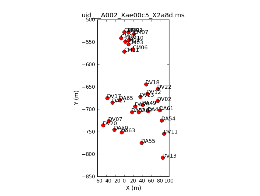
Now let's plot the antennas with plotants:
# In CASA
plotants(vis=mso, figfile='plotants.png')
Flagging Unnecessary Data
Some scans in the data were used by the online system for pointing and sideband ratio calibration. These scans are no longer needed, and we can flag them easily with flagdata by selecting on 'intent'.
#In CASA
flagdata(vis=mso, mode='manual', intent='*POINTING*,*SIDEBAND_RATIO*', flagbackup=False)
The averaged data of each spectrum window is not used, so we flagged the averaged data as a follow.
#In CASA
flagdata(vis=mso, mode='manual', spw='6,8,10,12', flagbackup=False)
We will then store the current flagging state for each dataset using the flagmanager:
#In CASA
flagmanager(vis=mso, mode='save', versionname='priori1')
A priori calibration
Tsys calibration of the calibrators
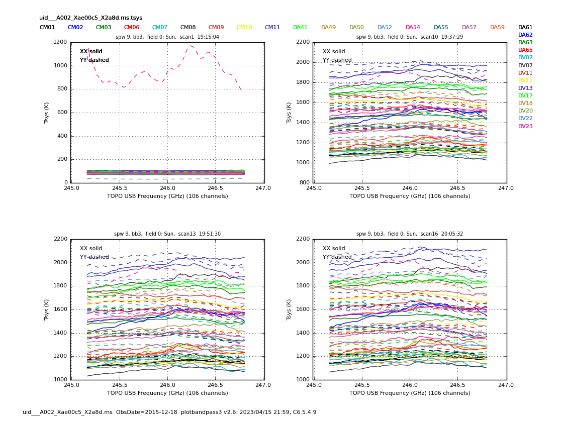
The System Temperature (Tsys) calibration gives a first-order correction for the atmospheric opacity as a function of time and frequency, and associates weights with each visibility that persist through imaging. The MS dataset contains Tsys measurements; the task gencal is used to generate a calibration table. Since the dataset obtained with TDM, the data in the channels near the both edges of the spectrum window (~10 channels) are flagged with flagdata. The plots for checking are created by the checkCalTable subroutine of the Analysis Utilities package and saved to a new directory uid___A002_Xae00c5_X2a8d.ms.tsys.plots (Figure 2).
#In CASA
gencal(vis=mso, caltable=mso+'.tsys', caltype='tsys')

flagdata(vis=mso+'.tsys', mode='manual', spw='5:0~9;116~127,7:0~9;116~127,9:0~9;116~127,11:0~9;116~127', flagbackup=False)

es.checkCalTable(mso+'.tsys', msName=mso, interactive=False)
The Tsys of DA54 antennas are significant large, from the plot. In the later part, we will flag the data of the antenna. Please ignore the data of the scan #1, because the scan is not done for ATM cal. The scan is used for the measurement of zero-signal level .
We will apply the Tsys calibration table to the data of the calibrators with the task applycal, which reads the specified gain calibration tables, applies them to the (raw) data column, and writes the calibrated results into the corrected column. For non-solar observations, we also apply the WVR (Water Vapor Radiometer) calibration table to data. However, we must NOT apply the WVR table to the solar data, because the WVR receivers at the Sun are saturated. We apply the Tsys calibration table to the data of the bandpass calibrator:
#In CASA
applycal(vis=mso, field='1', spw='5,7,9,11', gaintable=mso+'.tsys', gainfield='1', interp='linear,linear', calwt=True, flagbackup=False)
For normal ALMA observations, in between the science target scans, we would perform two adjacent scans of the phase calibrator: one with ATM intent, and one with PHASE intent. We would then apply the Tsys calibration table for the phase calibrator to itself.
The Sun is very dynamic, and the time variations of solar structures are one of the main scientific topics of solar physics. To observe such structures, the suspension of science scans are problematic. Therefore, to return to the Sun as quickly as possible, we do NOT perform ATM scans of the phase calibrator in between science scans, instead only observing PHASE intent scans (9,12,15,18).

However, the antenna temperature (Tant) of the Sun is not negligible and must be calibrated. To do this, we perform ATM scans of the blank sky near the Sun, 2 degrees from the Sun's center. Field 0 is used for all calibration scans, and is the center of the mosaic, as we will see later (Fields 3~150 are used for science scans only). The first subscan of science scans (11,14,17) are listed as Field 0, but include the "OBSERVE_TARGET#OFF_SOURCE" intent, which slews to the blank sky.

In this Science Verification observation, one scan of the phase calibrator has ATM intent (scan 7) before any science scans begin, but more recent solar observations do not include this. Scan 7 can be ignored.
For details, see Shimojo+ 2017, in particular Figure 4.
Therefore, we calibrate the Tsys of the phase calibrator (field='2') by applying the calibrations for the Sun (gainfield='0'), as follows:
#In CASA
applycal(vis=mso, field='2', spw='5,7,9,11', gaintable=mso+'.tsys', gainfield='0', interp='linear,linear', calwt=True, flagbackup=False)
You can use plotms to plot channel-averaged amplitudes as a function of time, comparing the DATA and CORRECTED columns after applying the Tsys correction. This way you can check that calibration has done what was expected, which is put the data onto the Kelvin temperature scale.
Tsys+Tant calibration of the Sun
The standard method of Tsys calibration cannot be applied to the data of the Sun, because the antenna temperature (Tant) of the Sun cannot be neglected for estimating the system equivalent flux density (SEFD). To estimate correct SEFD at the Sun, the solar observing sequence includes some special measurements, like the measurement of zero-signal level (scan 1). The subroutines for creating and applying Tsys+Tant calibration tables are prepared by the ALMA solar development team. They are part of the script we executed in the section #Import Tools and Scripts. For the Tsys+Tant calibration of the solar data, you will execute only the following command:
#In CASA
sol_ampcal_2(mso, mso+'.tsys', exisTbl=False, outCSV=True)
This process takes a long time. Depending on your machine, it may be between a couple hours and one day.
If you have already carried out the process before and there are the Tsys+Tant calibration tables (The directory name of the table includes “tsystant”), you can skip the generating of the tables using the following command.
Bug in Sun_reduction_util_6.5.4.py: underneath "if exisTbl == True:", scan = sciScan[i] should be scan = str(sciScan[i]).
#In CASA
sol_ampcal_2(mso, mso+'.tsys', exisTbl=True, outCSV=False)
Flagging after Tsys and Tsys+Tant calibration
Since we completed the Tsys and Tsys+Tant calibration, we can now flag the data that are not used for image synthesis. At first, the data of auto-correlation and atmosphere calibration are flagged with flagdata as follows:
#In CASA
flagdata(vis=mso, mode='manual', autocorr=True, flagbackup=False)
flagdata(vis=mso, mode='manual', intent='*ATMOSPHERE*', flagbackup=False)
Next are the spectral windows that are not used later:
#In CASA
flagdata(vis=mso, mode='manual', spw='0~4', flagbackup=False)
flagdata(vis=mso, mode='manual', spw='13~36', flagbackup=False)
The channels near both edges of the science spectral windows (~10 channels) are flagged:
#In CASA
flagdata(vis=mso, mode='manual', flagbackup=False, spw='5:0~9;116~127,7:0~9;116~127,9:0~9;116~127,11:0~9;116~127')
Some sub-scans at the start and end of the scientific scans are used to measure the sky with the settings optimized for the Sun. Since the data are used only for estimating the antenna temperatures at the Sun, we now flag the data:
#In CASA
mymsmd = createCasaTool(msmdtool)
mymsmd.open(mso)
sciScan = mymsmd.scansforintent('*OBSERVE_TARGET*')
mymsmd.done()

for i in range(0, len(sciScan)):
      subInf=aU.computeDurationOfScan(sciScan[i], vis=mso, returnSubscanTimes=True)
      subNum = subInf[1]
      flagdata(vis=mso, timerange=subInf[3][1], mode='manual', flagbackup=False)
      flagdata(vis=mso, timerange=subInf[3][2], mode='manual', flagbackup=False)
      flagdata(vis=mso, timerange=subInf[3][subNum-1], mode='manual', flagbackup=False)
      flagdata(vis=mso, timerange=subInf[3][subNum], mode='manual', flagbackup=False)
As mentioned in the section #Tsys calibration of the calibrators, the Tsys values of DA54 antennas are significantly large. Therefore, we flag the data of the antenna as follows:
#In CASA
flagdata(vis=mso, antenna='DA54', mode='manual', flagbackup=False)
Now we store the current flagging state using flagmanager:
#In CASA
flagmanager(vis=mso, mode='save', versionname='priori2')
Now split out the CORRECTED data column, retaining spectral windows 5,7,9,11. This will get rid of the extraneous spectral windows.
#In CASA
split(vis=mso, outputvis=mss, datacolumn='corrected', intent ='*BANDPASS*,*FLUX*,*PHASE*,*TARGET*', spw='5,7,9,11')
CAUTION: When we run split, the spws that we choose to keep will be re-indexed to 0,1,2,3.
Additional Data Inspection
Now let's inspect the split MS with plotms.
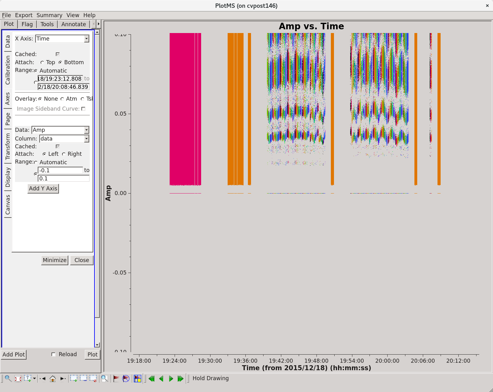
The solar data frequently include zero values in some channels. This is best seen with all plot averaging turned off, though it may take plotms a moment to load. We can restrict the Y axis to a small number since we are looking for pure zero values.
#In CASA
plotms(vis=mss,
       xaxis='time',
       yaxis='amp',
       coloraxis='field',
       plotrange=[0,0,-0.1,0.1]
       )
To avoid their influence, we flag the data using the “clip” mode of flagdata with “clipzeros=True” option.
#In CASA
flagdata(vis=mss, mode='clip', clipzeros=True, flagbackup=False)
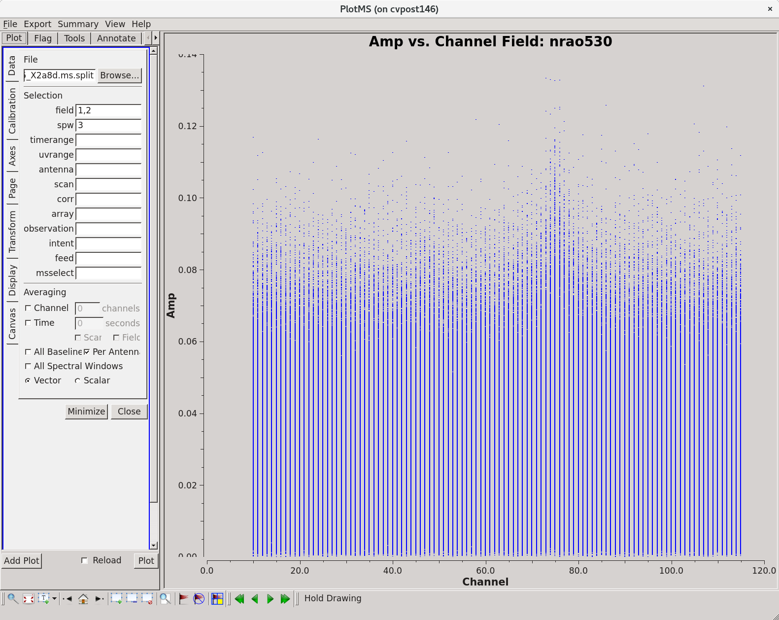
Now let's plot Amp vs Channel for our two calibrators.
#In CASA
plotms(vis=mss,
       field='1,2',
       spw='3',
       xaxis='channel',
       yaxis='amp',
       avgantenna=True,
       iteraxis='field'
       )
Valleys appear in spw 3. It shows the effect of the lines of the Earth's atmosphere. We need to flag the data.
#In CASA
flagdata(vis=mss, spw='3:68~85', mode='manual', flagbackup=False)
flagdata(vis=mss, spw='3:20~40', mode='manual', flagbackup=False)
Then, we store the current flagging state for each dataset using the flagmanager:
#In CASA
flagmanager(vis=mss, mode='save', versionname='initial')
Set up the Flux Calibration Model
It is very rare that a useful planet for the flux calibration is located near the Sun. Therefore, we usually use a quasar near the Sun as a flux calibrator. In these observations, there is no quasar with enough flux with the Mixer De-tuning mode except nrao530. Therefore, the flux calibrator is the same as the phase calibrator in these observation. We obtain the flux density and spectral index of nrao530 from the ALMA calibrator database.
#In CASA
intentSources = es.getIntentsAndSourceNames(mss)
ampCalId = intentSources['CALIBRATE_AMPLI']['id'] + intentSources['CALIBRATE_FLUX']['id']
calFieldNames = intentSources['CALIBRATE_AMPLI']['name'] + intentSources['CALIBRATE_FLUX']['name']

amp_cal_name = calFieldNames[1]
spwInfo = es.getSpwInfo(mss)
obs_freq = "%fGHz"%(spwInfo[0]['refFreq']/1e9)

date = aU.getObservationStartDate(mss)
date_obs = date.split()[0]
spw1_flux = aU.getALMAFlux(sourcename=amp_cal_name, date=date_obs, frequency=obs_freq)
You will see the following output in terminal:
Result using spectral index of -0.676873 for 231.000 GHz from 3.265 Jy at 97.500 GHz = 1.821049 +- 0.084762 Jy
Then, fill the model data column for nrao530 by providing this model to setjy.
#In CASA
setjy(vis=mss, field='2', spw='0,1,2,3', standard='manual', fluxdensity=[spw1_flux['fluxDensity'],0,0,0], spix=spw1_flux['spectralIndex'], reffreq=obs_freq, usescratch=True)
You will see the following output in the logger:
Flux density as a function of frequency (channel 0 of each spw):
  Frequency (GHz)    Flux Density (Jy, Stokes I)
     230.992         1.82116
     232.992         1.81056
     245.008         1.74997
     247.008         1.74037
Creating the Bandpass Calibration Table
The bandpass and gain calibrations are essentially the same as for non-solar data. First, we choose a reference antenna, then run gaincal on the bandpass calibrator to determine phase-only gain solutions. We will use solint='int' for the solution interval, which means that one gain solution will be determined for every integration time.
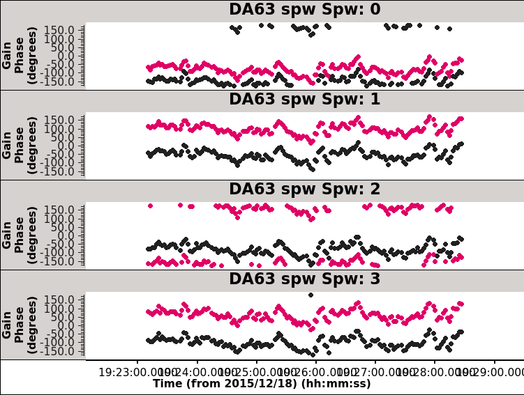
#In CASA
ref_ant = 'DA41'
gaincal(vis=mss, caltable=mss+'.pre_bandpass', field='1', scan='5', solint='int', refant=ref_ant, calmode='p')
Create plots to check the calibration table. These will be saved to a new directory uid___A002_Xae00c5_X2a8d.ms.split.pre_bandpass.plots.
#In CASA
es.checkCalTable(mss+'.pre_bandpass', msName=mss, interactive=False)
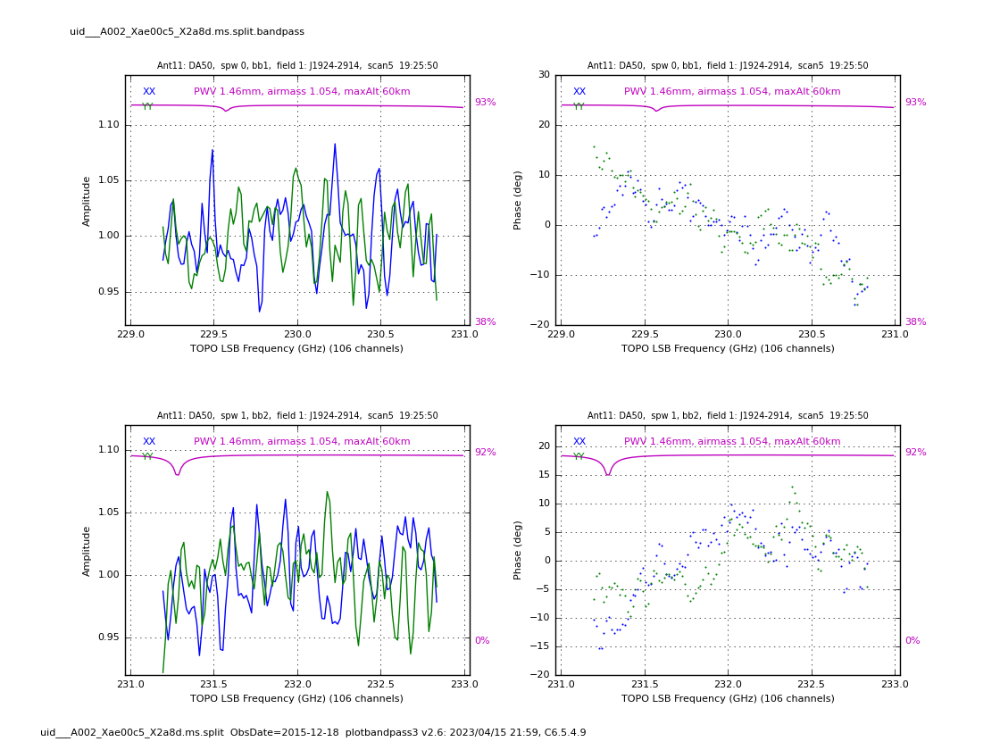
The plots look good. Next, create the bandpass calibration table. Since we apply the per-integration phase solutions on-the-fly, we can use solint='inf' to average the scan in time, resulting in higher signal-to-noise for our bandpass solution. You will see many warning reported about "insufficient unflagged antennas," which are for the edge channels we flagged so they are safe to ignore.
#In CASA
bandpass(vis=mss, caltable=mss+'.bandpass', field='1', scan='5', solint='inf', refant=ref_ant, solnorm=True, bandtype='B', gaintable=mss+'.pre_bandpass')
Check the bandpass calibration table using the plots created from the following command, which are saved into a new directory uid___A002_Xae00c5_X2a8d.ms.split.bandpass.plots.
#In CASA
es.checkCalTable(mss+'.bandpass', msName=mss, interactive=False)
Creating the Gain Calibration Tables
At first, we determine phase-only gain solutions of the calibrators with gaincal, applying the bandpass calibration table on-the-fly, using solint='int' for per-integration solutions. Then create the plots for checking, saved to uid___A002_Xae00c5_X2a8d.ms.split.phase_int.plots.
#In CASA
gaincal(vis=mss, caltable=mss+'.phase_int', field='1~2', solint='int', refant=ref_ant, gaintype='G', calmode='p', minsnr=3.0, gaintable=mss+'.bandpass')

es.checkCalTable(mss+'.phase_int', msName=mss, interactive=False)
Now apply both the bandpass and short phase solution tables on-the-fly to solve for amplitude-only gain solutions over the full scan time with solint='inf'. Plots are saved to uid___A002_Xae00c5_X2a8d.ms.split.ampli_inf.plots.
# In CASA
gaincal(vis=mss, caltable=mss+'.ampli_inf', field='1~2', solint='inf', refant=ref_ant, gaintype='G', calmode='a', minsnr=3.0, gaintable=[mss+'.bandpass', mss+'.phase_int'])

es.checkCalTable(mss+'.ampli_inf', msName=mss, interactive=False)
Usually, the gaintype is set to 'T' for nominal ALMA observations. For solar data, the gaintype is set to 'G', because the difference between the XX and YY images is used for estimating the noise level (see Section 4.2, Shimojo et al. 2017).
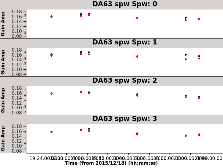
Next we use the flux calibrator (whose flux density was set in setjy above) to derive the flux density of the other calibrators with fluxscale. Note that the flux table REPLACES '.ampli_inf' in terms of future application of the calibration to the data, i.e., the flux table contains both the amplitude calibration and flux scaling. Unlike the two gaincal steps above, this is not an incremental table. Plots are saved to uid___A002_Xae00c5_X2a8d.ms.split.flux_inf.plots.
#In CASA
fluxscaleDict = fluxscale(vis=mss, caltable=mss+'.ampli_inf', fluxtable=mss+'.flux_inf', reference='2')

es.checkCalTable(mss+'.flux_inf', msName=mss, interactive=False)
You should see the following output:
Found reference field(s): nrao530
Found transfer field(s):  J1924-2914
Flux density for J1924-2914 in SpW=0 (freq=2.3e+11 Hz) is: 3.31068 +/- 0.0174892 (SNR = 189.299, N = 60)
Flux density for J1924-2914 in SpW=1 (freq=2.32e+11 Hz) is: 3.30137 +/- 0.016152 (SNR = 204.394, N = 60)
Flux density for J1924-2914 in SpW=2 (freq=2.46e+11 Hz) is: 3.16067 +/- 0.0180585 (SNR = 175.024, N = 60)
Flux density for J1924-2914 in SpW=3 (freq=2.48e+11 Hz) is: 3.14243 +/- 0.0205412 (SNR = 152.981, N = 60)
Fitted spectrum for J1924-2914 with fitorder=1: Flux density = 3.22814 +/- 0.002994 (freq=238.864 GHz) spidx: a_1 (spectral index) =-0.712504 +/- 0.0278242 covariance matrix for the fit:  covar(0,0)=7.85242e-06 covar(0,1)=9.80161e-05 covar(1,0)=9.80161e-05 covar(1,1)=0.0374698
Finally, we create the gain calibration table of phase-only gain solutions on the scan time, solint='inf'. Plots are saved to uid___A002_Xae00c5_X2a8d.ms.split.phase_inf.plots.

#In CASA
gaincal(vis=mss, caltable=mss+'.phase_inf', field='1~2', solint='inf', refant=ref_ant, gaintype='G', calmode='p', minsnr=3.0, gaintable=mss+'.bandpass')

es.checkCalTable(mss+'.phase_inf', msName=mss, interactive=False)
Applying the Calibration Tables
We apply the calibration solutions to each source individually with applycal, using the gainfield parameter to specify which calibrator's solutions should be applied from each of the calibration tables. We can leave gainfield blank when referencing the bandpass table, because this table has information derived only from the bandpass calibrator which will be applied to all sources.
Apply to the bandpass calibrator: the bandpass table; the short solint phase table, referencing the BP cal; and the flux table, referencing the BP cal.
#In CASA
applycal(vis=mss, field='1', gaintable=[mss+'.bandpass', mss+'.phase_int', mss+'.flux_inf'], gainfield=['', '1', '1'],
interp='linear,linear', calwt=True, flagbackup=False)
Apply to the phase calibrator: the bandpass table; the short solint phase table, referencing the phase cal; and the flux table, referencing the phase cal.
#In CASA
applycal(vis=mss, field='2', gaintable=[mss+'.bandpass', mss+'.phase_int', mss+'.flux_inf'], gainfield=['', '2', '2'],
interp='linear,linear', calwt=True, flagbackup=False)
Apply to the Sun: the bandpass table; the long solint phase table, referencing the phase cal; and the flux table, referencing the phase cal.
#In CASA
applycal(vis=mss, field='0, 3~150', gaintable=[mss+'.bandpass', mss+'.phase_inf', mss+'.flux_inf'], gainfield=['', '2', '2'],
interp='linear,linear', calwt=True, flagbackup=False)
Finally, split out the CORRECTED data column.
#In CASA
split(vis=mss, outputvis=msc, datacolumn='corrected')
Re-calculation of the direction
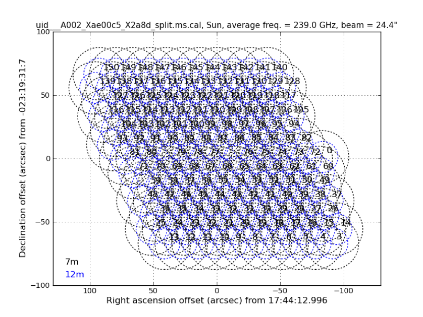
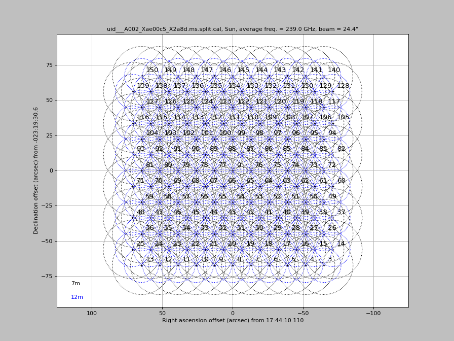
During most solar observations, the antennas are tracking a structure on the Sun according to the solar differential rotation. The image frame is fixed on the solar frame, but the frame is moving on the RA/Dec coordinate frame. If we do not correct for this, the pattern of pointing in the mosaic is a rhombus as shown in Figure 3, while the correct shape should be a square.
Plot the mosaic to see this:
The following command does not correctly create the plot as shown in Figure 3 at this time. Figure 3 is taken from a previous version of this guide.
#In CASA
au.plotmosaic(vis=msc, sourceid='Sun', figfile=msc+'.pointings.sun.before.png')
To correct the MOSAIC pattern, we re-calculate the coordinate of each field. First, we modify the coordinate of field='0' from the reference time using fixplanets task. The reference time has to be the time when the antennas are directed to field='0'.
#In CASA
reftime = '2015/12/18/19:49:00'
fixplanets(vis=msc, field='0', fixuvw=False, refant=ref_ant, reftime=reftime)
We define that the modified coordinate of field='0' is the reference coordinate, and re-calculate the coordinate of each field, as follows:
#In CASA
import math
pi = math.pi

tb.open(msc+'/FIELD', nomodify=True)
phsCenOff = tb.getcol("PHASE_DIR")
tb.close()

refRaDec = aU.rad2radec(phsCenOff[0][0][0], phsCenOff[1][0][0], prec=1, hmsdms=True, delimiter=' ')
for i in range(3, 151):
    raOff = phsCenOff[0][0][i] * 180. / pi * 60. *60.
    deOff = phsCenOff[1][0][i] * 180. / pi * 60. *60.
    offRaDec = aU.radec2deg(aU.radecOffsetToRadec(refRaDec, raOff, deOff, prec=1))
    offRaDecF = 'J2000 ' + aU.deg2radec(offRaDec[0], offRaDec[1], prec=1, hmsdms=True, delimiter=' ')
    fixplanets(vis=msc, field=str(i), fixuvw=False, direction=offRaDecF)

tb.open(msc+'/FIELD', nomodify=False)
tgt_refdir = tb.getcol("RefDir_Ref")
for id in range(3, len(tgt_refdir)):
    tb.putcell("RefDir_Ref", id, 21)
    tb.putcell("DelayDir_Ref", id, 21)
    tb.putcell("PhaseDir_Ref", id, 21)
tb.close()
Moreover, the direction in the pointing table has a bad influence on the coordinate system for image synthesis. We erase the pointing table as follows:
#In CASA
tb.open(msc+'/POINTING', nomodify=False)
a = tb.rownumbers()
tb.removerows(a)
tb.close()
Now plot the corrected mosaic:
#In CASA
au.plotmosaic(vis=msc, sourceid='Sun', figfile=msc+'.pointings.sun.after.png')