AIPS-Spectral Lines and Astrometry: Difference between revisions
No edit summary |
|||
| (104 intermediate revisions by 5 users not shown) | |||
| Line 1: | Line 1: | ||
<div style="text-align: justify;"> | |||
== Overview == | == Overview == | ||
A good resource for reducing basic VLBI data in AIPS can be found in [ | A good resource for reducing basic VLBI data in AIPS can be found in [http://www.aips.nrao.edu/TEXT/PUBL/COOKC.PS Appendix C] of the [http://www.aips.nrao.edu/cook.html AIPS Cookbook]. [http://www.aips.nrao.edu/TEXT/PUBL/COOK9.PS Chapter 9:Reducing VLBI Data in AIPS] of the AIPS Cookbook contains much more detail, but is best used as a reference. Details on the geodetic like calibration to improve phase referencing and astrometry can be found in [http://www.aips.nrao.edu/TEXT/PUBL/AIPSMEM110.PS AIPS Memo 110: Strategy for Removing Tropospheric and Clock Errors using DELZN.] In short, to obtain precise positions and good image quality with phase referencing in VLBI, two things are needed; a close calibrator to the target source to minimize atmospheric differences between the target and calibrator and a good correlator model. The VLBA correlator uses a model for the troposphere computed from seasonal models as well as the best estimates of the clocks, positions of each antenna, and earth orientation parameters. These major sources of error produce a systematic phase difference between the calibrator and target which limits the target positional accuracy and image quality. The troposphere model error, however, can be estimated by observing about ten calibrators over the sky over a 30-minute period, and then calculating the erroneous delay. So with this tutorial you will: | ||
*Calibrate the regular data all the way through imaging. | *Calibrate the regular data all the way through imaging. | ||
| Line 11: | Line 11: | ||
*Image the target and see an improvement over not doing the geodetic calibration. | *Image the target and see an improvement over not doing the geodetic calibration. | ||
This guide only | This guide only gives the important inputs to each task. The other inputs should be left at their defaults. An easy way to set all the inputs to the default in a task is to type "default ''taskname''". | ||
== AIPS == | == AIPS == | ||
| Line 17: | Line 17: | ||
For a comprehensive overview of AIPS see the [http://www.aips.nrao.edu/CookHTML/CookBook.html AIPS COOKBOOK], especially [http://www.aips.nrao.edu/CookHTML/CookBookch3.html#x20-240003 Chapter 3:Basic AIPS Utilities] and [http://www.aips.nrao.edu/CookHTML/CookBookch12.html#x107-31300012 Chapter 12:AIPS for the More Sophisticated User]for the basics. [http://www.aips.nrao.edu/CookHTML/CookBookch9.html#x87-2010009 Chapter 9:Reducing VLBI Data in AIPS] is the chapter explaining VLBI data reduction, but it is rather overwhelming so [http://www.aips.nrao.edu/CookHTML/CookBookap3.html#x171-401000C Appendix C:A Step-by-Step Recipe for VLBA Data Calibration in AIPS] is recommended as a first step. However, below I summarize some useful commands (in parenthesis are the short form of the command): | For a comprehensive overview of AIPS see the [http://www.aips.nrao.edu/CookHTML/CookBook.html AIPS COOKBOOK], especially [http://www.aips.nrao.edu/CookHTML/CookBookch3.html#x20-240003 Chapter 3:Basic AIPS Utilities] and [http://www.aips.nrao.edu/CookHTML/CookBookch12.html#x107-31300012 Chapter 12:AIPS for the More Sophisticated User]for the basics. [http://www.aips.nrao.edu/CookHTML/CookBookch9.html#x87-2010009 Chapter 9:Reducing VLBI Data in AIPS] is the chapter explaining VLBI data reduction, but it is rather overwhelming so [http://www.aips.nrao.edu/CookHTML/CookBookap3.html#x171-401000C Appendix C:A Step-by-Step Recipe for VLBA Data Calibration in AIPS] is recommended as a first step. However, below I summarize some useful commands (in parenthesis are the short form of the command): | ||
*getname (getn) ''catalog #'': get the name of catalog # and | *getname (getn) ''catalog #'': get the name of catalog # and fill in INNAME, INCLASS and INSEQ. Other similar: geton (get outname); get2n (get in2name); get3n (getin3name) etc.. | ||
*input (inp) ''taskname'': show the inputs of taskname. | *input (inp) ''taskname'': show the inputs of taskname. | ||
*tget ''taskname'': get a task and fill in the inputs of the last time the task was run, one of the most useful commands in AIPS. | *tget ''taskname'': get a task and fill in the inputs of the last time the task was run, one of the most useful commands in AIPS. | ||
*ucat (uc): list uvdata catalog. | *ucat (uc): list uvdata catalog. | ||
*mcat (mc): list map catalog. | *mcat (mc): list map catalog. | ||
*tvlod (tvlo): load | *pca: list all catalogs. | ||
*tvlod (tvlo): load a map onto the TV. | |||
*tvinit (tvin): initialize and clear TV. | *tvinit (tvin): initialize and clear TV. | ||
*imhead (imh): Print the file header (this can be used on both uv data and images despite the name). This will list informative things like the date of observation and the number and types of tables attached to the data. | *imhead (imh): Print the file header (this can be used on both uv data and images despite the name). This will list informative things like the date of observation and the number and types of tables attached to the data. | ||
== Getting the Data == | == Getting the Data == | ||
To obtain the data, right click on these file names below and select "Save Link As..." | To obtain the data, right click on these file names below and select "Save Link As..." . Put the data into your $FITS area, which should be an AIPS area that is automatically set up when you install AIPS. | ||
*[ | *[http://www.aips.nrao.edu/FITS/VLBA/BM272HC.fits BM272HC.fits] (12 GB): Data containing target and calibrators. | ||
*[ | *[http://www.aips.nrao.edu/FITS/VLBA/BM272HC_geodetic.fits BM272HC_geodetic.fits] (0.3 GB): Data containing geodetic block. These are observations of many calibrators around the sky. | ||
If that doesn't work you can also ftp the data using anonymous ftp: | If that doesn't work you can also ftp the data using anonymous ftp: | ||
| Line 37: | Line 38: | ||
*mget *.fits | *mget *.fits | ||
The geodetic blocks are in a different file from the target because they have very different frequency setups. The geodetic block | The geodetic blocks are in a different file from the target because they have very different frequency setups. The geodetic block is required to have widely spaced frequencies with a single polarization in order to measure the multi-band delay (MBD). The target dataset is dual polarization (important since the source is circularly polarized) and frequencies that are continuous. '''MAKE SURE YOU ARE RUNNING THE CORRECT TASK ON THE CORRECT DATASET!''' | ||
== About the Data == | == About the Data == | ||
| Line 43: | Line 44: | ||
This is an observation of water masers in star-forming region IRAS 00420+5530 and involves phase referencing. The sources in the the BM272HC.fits dataset are as follows: | This is an observation of water masers in star-forming region IRAS 00420+5530 and involves phase referencing. The sources in the the BM272HC.fits dataset are as follows: | ||
*AFGL2591 - phase calibrator/target ( | *AFGL2591 - phase calibrator/target (maser source for which the position is desired) | ||
*J2007+4029, 20330+40003, 20327+40396, 20324+40574 - calibrators that are phase referenced to AFGL2591 (note that only J2007+4029 and 20330+40003 are detected). | *J2007+4029, 20330+40003, 20327+40396, 20324+40574 - calibrators that are phase referenced to AFGL2591 (note that only J2007+4029 and 20330+40003 are detected). | ||
*3C345A, 3C454.3A - Bright, well known quasars, used as fringe finders and bandpass calibrators | *3C345A, 3C454.3A - Bright, well known quasars, used as fringe finders and bandpass calibrators | ||
| Line 95: | Line 96: | ||
# default listr | # default listr | ||
# getn BM272HC.UVDATA.1 file; in other words getn 1 | # getn '''BM272HC.UVDATA.1 file'''; in other words ''getn 1'' | ||
# optype 'scan' | # optype 'scan' | ||
# docrt 1 | # docrt 1 | ||
| Line 109: | Line 110: | ||
# run vlbautil | # run vlbautil | ||
If you get a BLEW CORE or other similar error message, you have filled your procedure memory (VLBAUTIL is very large and loading it three times will do this). To fix it type restore 0 then reload VLBAUTIL | If you get a BLEW CORE or other similar error message, you have filled your procedure memory (VLBAUTIL is very large and loading it three times will do this). To fix it type "restore 0" then reload VLBAUTIL | ||
=== Calibrate Ionospheric Delay === | === Calibrate Ionospheric Delay === | ||
| Line 120: | Line 121: | ||
# vlbatecr ➜ to run VLBATECR | # vlbatecr ➜ to run VLBATECR | ||
=== Fix | === Fix Earth Orientation Parameters === | ||
Fix earth orientation parameters by running [http://www.aips.nrao.edu/cgi-bin/ZXHLP2.PL?VLBAEOPS '''VLBAEOPS''']. | Fix earth orientation parameters by running [http://www.aips.nrao.edu/cgi-bin/ZXHLP2.PL?VLBAEOPS '''VLBAEOPS''']. | ||
| Line 148: | Line 149: | ||
# stokes 'half' | # stokes 'half' | ||
# refant 2 | # refant 2 | ||
# gainuse | # gainuse 0 | ||
# solint -1 | # solint -1 | ||
# dotv 1 | # dotv 1 | ||
| Line 168: | Line 169: | ||
Find and remove instrumental delay by running [http://www.aips.nrao.edu/cgi-bin/ZXHLP2.PL?VLBAMPCL '''VLBAMPCL''']. | Find and remove instrumental delay by running [http://www.aips.nrao.edu/cgi-bin/ZXHLP2.PL?VLBAMPCL '''VLBAMPCL''']. | ||
[[Image:POSSMafterMPCL.png|250px|thumb|right|'''Figure 2''' <br /> | [[Image:POSSMafterMPCL.png|250px|thumb|right|'''Figure 2''' <br /> Plots for source 3C345A which show the amplitude (bottom panel) and corrected phases (top panel), for each IF in both polarizations.]] | ||
#default vlbampcl | #default vlbampcl | ||
#getn 1 | #getn 1 | ||
#calsour '3C345A' | #calsour '3C345A' ' ➜ strongest source. | ||
#timer 0 07 35 28 0 | #timer 0 07 35 28 0 07 37 09 ➜ scan with good fringes we found in POSSM plots. | ||
#refant 2 ➜ choose reference antenna from in the middle of array, FD (antenna 2) is a good choice. | #refant 2 ➜ choose reference antenna from in the middle of array, FD (antenna 2) is a good choice. | ||
#gainu | #gainu 0 ➜ apply highest CL table. | ||
#inp | #inp | ||
#vlbampcl | #vlbampcl | ||
| Line 189: | Line 190: | ||
FRING1: Adjusting solutions to a common reference antenna | FRING1: Adjusting solutions to a common reference antenna | ||
</pre> | </pre> | ||
For this step there ''must be no failed solutions'' | |||
For this step there ''must be no failed solutions''. Failed solutions in this step means that whichever antenna the failed solution was on is deleted from your data. For this data, because there are 10 antennas, 2 polarizations and 4 spectral windows (IFs), there should be "80 good solutions". | |||
*check solutions in POSSM, the jumps in phase between the IFs should be gone. The phases may also be flattened. | *check solutions in POSSM, the jumps in phase between the IFs should be gone. The phases may also be flattened. | ||
| Line 222: | Line 224: | ||
# go | # go | ||
The solutions should look like a reasonable fit of the bandpass shape. | Figure 3 shows the plots generated by POSSM. The solutions should look like a reasonable fit of the bandpass shape. | ||
=== Apply Amplitude Corrections === | === Apply Amplitude Corrections === | ||
| Line 243: | Line 245: | ||
# dotv 1 | # dotv 1 | ||
# inext 'cl' | # inext 'cl' | ||
# invers | # invers 0 | ||
# opty 'amp' | # opty 'amp' ➜ Plot amplitudes. | ||
# nplots 10 | # nplots 10 | ||
# opco 'alsi' | # opco 'alsi' ➜ Plot all IFs and Stokes. | ||
# do3col 1 | # do3col 1 ➜ Use 3-color symbols. | ||
# inp | # inp | ||
# tvin ➜ | # tvin ➜ tvinitialize clears the tv before plotting. Otherwise you will get a mess as the table is plotted over the bandpass plot from before. | ||
# go | # go | ||
Figure 4 shows the amplitude gains change over time as the sources rise and set, with higher gains at lower elevations | Figure 4 shows the amplitude gains change over time as the sources rise and set, with higher gains at lower elevations. Because 3C345 and 3C454.3 are so strong, they will increase the gains. The different IFs and polarizations (RR and LL in this case) are shown as different colors. | ||
=== Correct Phases for Parallactic Angles === | === Correct Phases for Parallactic Angles === | ||
Correct phases for parallactic angle effects with [http://www.aips.nrao.edu/cgi-bin/ZXHLP2.PL?VLBAPANG '''VLBAPANG''']. | |||
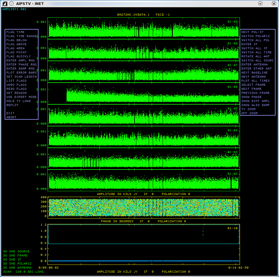
[[Image:EDITRbefore.png|250px|thumb|right|'''Figure 5''' <br /> EDITR plot showing a high data point for baselines 01-10 that we will need to flag.]] | |||
[[Image:EDITRbefore.png|250px|thumb|right|'''Figure 5''' <br /> | |||
# default vlbapang | # default vlbapang | ||
| Line 267: | Line 268: | ||
=== Manually Edit Data === | === Manually Edit Data === | ||
[[Image:EDITRflagtime.png|250px|thumb|right|'''Figure 6''' <br /> | [[Image:EDITRflagtime.png|250px|thumb|right|'''Figure 6''' <br /> EDITR plot showing the cutoff area for the FLAG ABOVE option. Every data point above the cutoff line will be flagged.]] | ||
[[Image:EDITRaftreplot.png|250px|thumb|right|'''Figure 7''' <br /> A " | [[Image:EDITRaftreplot.png|250px|thumb|right|'''Figure 7''' <br /> A "REPLOT" of baseline 01-10, after flagging of the high data point and re-scaling.]] | ||
Edit the data using [http://www.aips.nrao.edu/cgi-bin/ZXHLP2.PL?EDITR '''EDITR'''] on each source separately. | Edit the data using [http://www.aips.nrao.edu/cgi-bin/ZXHLP2.PL?EDITR '''EDITR'''] on each source separately. | ||
| Line 283: | Line 284: | ||
# outfgver 1 | # outfgver 1 | ||
# antuse 1 2 3 4 5 6 7 8 9 10 ➜ to plot all the baselines to one antenna at the same time. | # antuse 1 2 3 4 5 6 7 8 9 10 ➜ to plot all the baselines to one antenna at the same time. | ||
# source <nowiki>'AFGL2591''</nowiki> ➜ run on one source at a time | |||
# inp | |||
# go | |||
Again look in your terminal window for intructions: | |||
Again look in | |||
<pre> | <pre> | ||
EDITR1: Press buttons A, B, or C to choose an operation | |||
EDITR1: Press button D for on-line help | EDITR1: Press button D for on-line help | ||
</pre> | </pre> | ||
Note that the data looks great but there are a few high points we'll want to flag. The data we want to flag is found on baseline 01-10 as seen in Figure 5. Click "NEXT BASELINE" found on the menu to the right and press "B" until baseline 01-10 is plotted in the edit window at the bottom of the display . We will now flag the high points with flagging options found on the left menu. Click "FLAG ABOVE" and hit B. Your mouse cursor should shift to the edit window. In the terminal window you will now see instructions for FLAG ABOVE: | |||
<pre> | <pre> | ||
EDITR1: Hit buttons A or B to flag high fluxes and continue | EDITR1: Hit buttons A or B to flag high fluxes and continue | ||
| Line 301: | Line 300: | ||
EDITR1: Hit button D to return to menu with no more flagging | EDITR1: Hit button D to return to menu with no more flagging | ||
</pre> | </pre> | ||
Choose where to place your cutoff line as seen in Figure 6. Every data point above this line will be flagged. Press "C" to flag the high fluxes and return to the menu. The data points should now be highlighted white. To view the results of the flagging, we can generate a new plot by clicking "REPLOT" and pressing B. The plot will update without the high data points as seen in Figure 7. There are two more baselines with similar problems. Click NEXT ANTENNA and button B repeatedly to examine all of the data. When bad points are found, click NEXT BASELINE and button B until the offending baseline appears in the edit window, and then click FLAG ABOVE with button B to remove the bad samples. Finally, on the left menu, click on "EXIT" then press B. This will write the flags to a new flagging table (FG) which we can later apply to the data. | |||
Now plot the other sources and inspect. | |||
*20330+40003: | *20330+40003: | ||
| Line 310: | Line 313: | ||
*#go | *#go | ||
EDITR plots both amplitudes and phases, so this is a good way to just look at your data. If you plot the phases on all the baselines, note that you can see coherent phases on J2007+4029, but not the other two sources. AFGL2591 has strong masers that fringe, but '''EDITR''' is plotting all the channels averaged. | |||
=== Backing up Your Calibration === | |||
We will want to save the calibration up to this point with [http://www.aips.nrao.edu/cgi-bin/ZXHLP2.PL?TASAV '''TASAV''']. TASAV makes a new file with all your calibration tables, this is very useful because it contains everything you need to recalibrate your data in a very compact and portable form. It is also a good idea to do this before you do anything you are unsure about or will change important tables (AN, SU) in ways that are hard to change them back. In the next step we are changing the SU table. | |||
We will want to save the calibration up to this point with [http://www.aips.nrao.edu/cgi-bin/ZXHLP2.PL?TASAV '''TASAV''']. TASAV makes a new file with all your calibration tables, this is very useful because it contains everything you need to recalibrate your data in a very compact form. It is also a good idea to do this before you do anything you are unsure about or will change important tables (AN, SU) in ways that are hard to change them back. In the next step we are changing the SU table. | |||
# default tasav | # default tasav | ||
| Line 334: | Line 335: | ||
AIPS 1: 3 1099 BM272HC .TASAV . 1 UV 07-APR-17 16:19:59 | AIPS 1: 3 1099 BM272HC .TASAV . 1 UV 07-APR-17 16:19:59 | ||
</pre> | </pre> | ||
Note that you now have a third catalog entry which TASAV automtically named BM272HC.TASAV.1. This uv data file has 1 visibility and all the tables attached to BM272HC.UVDATA.1. | Note that you now have a third catalog entry which TASAV automtically named BM272HC.TASAV.1. This uv data file has 1 visibility and all the tables attached to BM272HC.UVDATA.1. Lets look at the TASAVed file.: | ||
#getn 3 | |||
#imh | |||
You should get something that looks like: | |||
<pre> | |||
AIPS 1: Image=MULTI (UV) Filename=BM272HC .TASAV . 1 | |||
AIPS 1: Telescope=VLBA Receiver= | |||
AIPS 1: Observer=BM272 User #= 1099 | |||
AIPS 1: Observ. date=13-MAY-2009 Map date=14-APR-2017 | |||
AIPS 1: # visibilities 1 Sort order TB | |||
AIPS 1: Rand axes: UU-L-SIN VV-L-SIN WW-L-SIN TIME1 SUBARRAY | |||
AIPS 1: SOURCE FREQSEL INTTIM GATEID CORR-ID ANTENNA1 | |||
AIPS 1: ANTENNA2 | |||
AIPS 1: ---------------------------------------------------------------- | |||
AIPS 1: Type Pixels Coord value at Pixel Coord incr Rotat | |||
AIPS 1: COMPLEX 3 1.0000000E+00 1.00 1.0000000E+00 0.00 | |||
AIPS 1: STOKES 2 -1.0000000E+00 1.00 -1.0000000E+00 0.00 | |||
AIPS 1: FREQ 256 2.2217920E+10 1.00 3.1250000E+04 0.00 | |||
AIPS 1: IF 4 1.0000000E+00 1.00 1.0000000E+00 0.00 | |||
AIPS 1: RA 1 00 00 00.000 1.00 0.000000 0.00 | |||
AIPS 1: DEC 1 00 00 00.000 1.00 0.000000 0.00 | |||
AIPS 1: ---------------------------------------------------------------- | |||
AIPS 1: Coordinate equinox 2000.00 | |||
AIPS 1: Maximum version number of extension files of type HI is 1 | |||
AIPS 1: Maximum version number of extension files of type FQ is 1 | |||
AIPS 1: Maximum version number of extension files of type CT is 1 | |||
AIPS 1: Maximum version number of extension files of type OB is 1 | |||
AIPS 1: Maximum version number of extension files of type AN is 1 | |||
AIPS 1: Maximum version number of extension files of type CL is 8 | |||
AIPS 1: Maximum version number of extension files of type CQ is 1 | |||
AIPS 1: Maximum version number of extension files of type GC is 1 | |||
AIPS 1: Maximum version number of extension files of type IM is 1 | |||
AIPS 1: Maximum version number of extension files of type MC is 1 | |||
AIPS 1: Maximum version number of extension files of type PC is 1 | |||
AIPS 1: Maximum version number of extension files of type SU is 1 | |||
AIPS 1: Maximum version number of extension files of type TY is 1 | |||
AIPS 1: Maximum version number of extension files of type WX is 1 | |||
AIPS 1: Maximum version number of extension files of type SN is 4 | |||
AIPS 1: Maximum version number of extension files of type BP is 1 | |||
AIPS 1: Maximum version number of extension files of type FG is 1 | |||
</pre> | |||
Note that there are 8 calibration (CL) tables and 4 solution (SN) tables. As well as numerous other tables with information about your data (history (HI), frequency (FQ), antenna (AN), system temperature (TY), bandpass (BP), flag (FG)...). | |||
=== Apply Correction to CL Table === | === Apply Correction to CL Table === | ||
We will now shift the position of AFGL2591 with [http://www.aips.nrao.edu/cgi-bin/ZXHLP2.PL?CLCOR '''CLCOR''']. The observed/correlated position of AFGL2591 was quite wrong and shifting a large distance in the image plane is imprecise, therefore it is important to shift the uv-data with either '''CLCOR''' or [http://www.aips.nrao.edu/cgi-bin/ZXHLP2.PL?UVFIX '''UVFIX''']. Normally you would reduce and image the data to find the shift. | |||
# default clcor | # default clcor | ||
# getn 1 | # getn 1 | ||
# sour 'AFGL2591'' | # sour 'AFGL2591' ' | ||
# gainver 8 | # gainver 8 | ||
# gainuse 9 | # gainuse 9 | ||
# opcode 'antp' | # opcode 'antp' | ||
# clcorprm(5)= 0.009 | # clcorprm(5)= 0.009 ➜ Correction in RA direction in seconds of arc. | ||
# clcorprm(6)=-0.129 | # clcorprm(6)=-0.129 ➜ Correction in Dec direction in seconds of arc. | ||
# inp | # inp | ||
# go | # go | ||
| Line 354: | Line 396: | ||
=== Apply Calibrations === | === Apply Calibrations === | ||
Apply all calibration up to this point and copy out IF#3 with [http://www.aips.nrao.edu/cgi-bin/ZXHLP2.PL?SPLAT '''SPLAT''']. The masers are in the 3rd IF and we will be fringe fitting on that maser so we should get rid of the other IFs. We could have gotten rid of the other 3 IFs earlier, but I kept them around for two reasons, 1) I wanted you to see what more than one IF looked like in displays and editing since most of the data you will receive will be more than | Apply all calibration up to this point and copy out IF#3 with [http://www.aips.nrao.edu/cgi-bin/ZXHLP2.PL?SPLAT '''SPLAT''']. | ||
The masers are in the 3rd IF and we will be fringe fitting on that maser so we should get rid of the other IFs. We could have gotten rid of the other 3 IFs earlier, but I kept them around for two reasons, 1) I wanted you to see what more than one IF looked like in displays and editing, since most of the data you will receive will be more than one IF; and 2) it is a good idea to apply the calibration after the position shift, but before global fringe fitting and the zenith delay correction. | |||
# default splat | # default splat | ||
| Line 386: | Line 430: | ||
# tget possm | # tget possm | ||
# getn 4 | # getn 4 | ||
# sour 'AFGL2591'' | # sour 'AFGL2591' ' | ||
# base 2 0 | # base 2 0 | ||
# gainu 0 | # gainu 0 | ||
# solint -1 | # solint -1 | ||
# doband -1 | # doband -1 | ||
# docal -1 | |||
# aparm 0, 1, 0, 0, -180, 180, 0, 0, 1 | # aparm 0, 1, 0, 0, -180, 180, 0, 0, 1 | ||
# dotv 1 | # dotv 1 | ||
| Line 400: | Line 445: | ||
We really only need to look at one spectrum for this, so you can hit "D" right away or go through a few plots to see how the spectrum changes a bit from baseline to baseline. | We really only need to look at one spectrum for this, so you can hit "D" right away or go through a few plots to see how the spectrum changes a bit from baseline to baseline. | ||
Figure 8 shows that the maser is strongest in channel 145. | Figure 8 shows that the maser is strongest in channel 145 on a baseline FD-HN. | ||
=== Fringe Fit the Data === | === Fringe Fit the Data === | ||
Perform a global fringe fit with [http://www.aips.nrao.edu/cgi-bin/ZXHLP2.PL?FRING '''FRING''']. The following steps through imaging are not strictly necessary since we will have to redo them once the geodetic calibration is done, but is an excellent way to check the calibration up to this point is correct. | Perform a global fringe fit with [http://www.aips.nrao.edu/cgi-bin/ZXHLP2.PL?FRING '''FRING''']. The following steps through imaging are not strictly necessary since we will have to redo them once the geodetic calibration is done, but is an excellent way to check that the calibration up to this point is correct. | ||
# default fring | # default fring | ||
# getn 4 | # getn 4 | ||
# calsour 'AFGL2591'' ➜ do a global fringe fit on maser. | # calsour 'AFGL2591' ' ➜ do a global fringe fit on maser. | ||
# bchan 145;echan 145 | # bchan 145;echan 145 | ||
# refant 2 | # refant 2 | ||
| Line 417: | Line 462: | ||
# go | # go | ||
You should look at the number of good and failed solutions: | |||
<pre> | |||
FRING1: Found 4506 good solutions | |||
FRING1: Failed on 34 solutions | |||
FRING1: Adjusting solutions to a common reference antenna | |||
</pre> | |||
You should get something similar but not necessarily exactly the same numbers of good and failed solutions. A small percentage of failed solutions are fine at this point. | |||
Hint: We will have to do this exact same step after doing the zenith delay calibration so it is helpful to save the inputs to '''FRING'''. This can be done with [http://www.aips.nrao.edu/cgi-bin/ZXHLP2.PL?VNUM '''vnum'''] and [http://www.aips.nrao.edu/cgi-bin/ZXHLP2.PL?VPUT '''vput''']. | Hint: We will have to do this exact same step after doing the zenith delay calibration so it is helpful to save the inputs to '''FRING'''. This can be done with [http://www.aips.nrao.edu/cgi-bin/ZXHLP2.PL?VNUM '''vnum'''] and [http://www.aips.nrao.edu/cgi-bin/ZXHLP2.PL?VPUT '''vput''']. | ||
| Line 423: | Line 474: | ||
# vnum 1; vput fring | # vnum 1; vput fring | ||
=== | === Apply FRING solutions from AFGL2591 to Calibrators === | ||
Interpolate the fringe solutions with [http://www.aips.nrao.edu/cgi-bin/ZXHLP2.PL?CLCAL '''CLCAL''']. | Note that this is "phase referencing", you are getting phases on one source and applying them to another, nearby source. However the way we are doing it here is a little backwards, in most situations your target it too faint to use in FRING and you run FRING on one of the calibrators and apply those phases to your target. Here we are using the target maser in FRING because it is stronger and applying it to the calibrators because we care about positions. In this case any shift in the position of the calibrators will indicate that AFGL2591 has moved. Interpolate the fringe solutions with [http://www.aips.nrao.edu/cgi-bin/ZXHLP2.PL?CLCAL '''CLCAL''']. | ||
# default clcal | # default clcal | ||
| Line 431: | Line 482: | ||
# gainv 1 ➜ CL table with all the calibration. | # gainv 1 ➜ CL table with all the calibration. | ||
# gainu 2 ➜ CL table to write next step of calibration in. | # gainu 2 ➜ CL table to write next step of calibration in. | ||
# snver 1 ➜ | # snver 1 ➜ contains final fringe fit. | ||
# interpol '2PT' ➜ use 2PT interpolation. | # interpol '2PT' ➜ use 2PT interpolation. | ||
# refant 2 | # refant 2 | ||
# sour 'AFGL2591' '20330+40003' 'J2007+4029' ➜ sources to which to apply calibration. | # sour 'AFGL2591' '20330+40003' 'J2007+4029' ➜ sources to which to apply calibration. | ||
# calsour 'AFGL2591'' ➜ phase calibrator, phases will be applied from AFGL2591 to itself, 20330+40003 and J2007+4029. | # calsour 'AFGL2591' ' ➜ phase calibrator, phases will be applied from AFGL2591 to itself, 20330+40003 and J2007+4029. | ||
# inp | # inp | ||
# go | # go | ||
| Line 476: | Line 527: | ||
# default imagr | # default imagr | ||
# getn 5 | # getn 5 | ||
# bchan 125; echan 150; nchav 1; ➜ image channels | # bchan 125; echan 150; nchav 1; ➜ image channels 125-150. | ||
# cell 3e-5; imsi 1024 ➜ cell size of 0.03 mas; image size of 1024x1024. | # cell 3e-5; imsi 1024 ➜ cell size of 0.03 mas; image size of 1024x1024. | ||
# dotv 1; niter 1000 ➜ do interactive clean; with 1000 iterations. | # dotv 1; niter 1000 ➜ do interactive clean; with 1000 iterations. | ||
# im2parm 10 6 9 0.5 ➜ autoboxing, only do 10 boxes per major cycle; find islands with > 6*rms; box is accepted if peak > 9*rms; box is accepted if its peak brightness is >0.5*max residual. | |||
# inp | # inp | ||
# go | # go | ||
You can | '''HINT:''' The first few channels will not have any masers, just hit "STOP CLEANING" (and "A" to select, again look at the terminal for instructions) until you see some emission. Hit TVPSEUDO (and "A"), then "D" immediately to get color rather than grey scale. If you want to clean interactively, then click CONTINUE CLEAN (and "A"); if you want to add boxes use REBOX ("A"); when you are happy with the cleaning you can go to the next channel by clicking STOP CLEANING ("A"). You can turn off interactive clean by clicking TURN OFF DOTV ("A"). However, the appropriate stopping point in each channel varies both in terms of number of iterations and lowest believable flux, | ||
so you should interact with each channel patiently. Once IMAGR is done, you can do a mcat (mc for short) to look at the maps in your catalog: | |||
#mc | |||
<pre> | |||
AIPS 1: Catalog on disk 1 | |||
AIPS 1: Cat Usid Mapname Class Seq Pt Last access Stat | |||
AIPS 1: 8 1099 AFGL2591 .IBM001. 1 MA 14-APR-17 10:58:28 | |||
AIPS 1: 9 1099 AFGL2591 .ICL001. 1 MA 14-APR-17 10:58:28 | |||
</pre> | |||
Note that you have made two files, a "dirty beam" (the IBM001 file) and a cleaned map (ICL001). | |||
Look at cube with AFGL2591 [http://www.aips.nrao.edu/cgi-bin/ZXHLP2.PL?TVMOVIE '''TVMOVIE'''] (getn 9; tvmovie). Then collapse the cube with [http://www.aips.nrao.edu/cgi-bin/ZXHLP2.PL?SQASH '''SQASH'''] | |||
# default sqash | |||
# getn 9 | |||
# bdrop 3 | |||
# dparm 1 0 | |||
# go | |||
SQASH will produce another map in your catalog: | |||
#mc | |||
<pre> | |||
AIPS 1: Catalog on disk 1 | |||
AIPS 1: Cat Usid Mapname Class Seq Pt Last access Stat | |||
AIPS 1: 8 1099 AFGL2591 .IBM001. 1 MA 14-APR-17 10:58:28 | |||
AIPS 1: 9 1099 AFGL2591 .ICL001. 1 MA 14-APR-17 11:02:50 | |||
AIPS 1: 10 1099 AFGL2591 .SQASH . 1 MA 14-APR-17 11:02:50 | |||
</pre> | |||
''' | To look at it use [http://www.aips.nrao.edu/cgi-bin/ZXHLP2.PL?TVLOD '''TVLOD'''] (getn 10; tvin; tvlo). Use [http://www.aips.nrao.edu/cgi-bin/ZXHLP2.PL?TVPSEUDO '''TVPSEUDO'''] to put it into color (tvps). You can use your mouse to manipulate the colors, looking again at your terminal for instructions. Hit "D" once it looks the way you want. Figure 9 shows the SQASH result. | ||
=== Create More Images === | === Create More Images === | ||
| Line 500: | Line 572: | ||
# getn 6 or 7 | # getn 6 or 7 | ||
# bchan 0; echan 0; nchav 256; ➜ average all channels. | # bchan 0; echan 0; nchav 256; ➜ average all channels. | ||
# imsi 2048 ➜ larger image size because sources might not be at center of field. | # cell 3e-5;imsi 2048 ➜ larger image size because sources might not be at center of field. | ||
# im2parm 10 6 9 0.5 ➜ autoboxing again | |||
# dotv 1; niter 1000 ➜ do interactive clean; with 1000 iterations. | # dotv 1; niter 1000 ➜ do interactive clean; with 1000 iterations. | ||
# inp | # inp | ||
# go | # go | ||
Figure 10 shows the end result of running '''IMAGR'''. | Here I would check that the autobox looks OK (It should just be around the the obvious emission) and then hit TURN OFF DOTV ("A"). Figure 10 shows the end result of running '''IMAGR''' on J2007+4029 (getn 6). To image 20330+40003 you will need to set IMSIZE to 8192. The assumed coordinate for this source was not entirely correct. | ||
''' | [[Image:IMAGEJ2007before.png|250px|thumb|right|'''Figure 10''' <br /> A radio image of J2007+4029.]] | ||
Now do an mcat to see the maps we have created: | |||
#mc | |||
<pre> | |||
AIPS 1: Catalog on disk 1 | |||
AIPS 1: Cat Usid Mapname Class Seq Pt Last access Stat | |||
AIPS 1: 8 1099 AFGL2591 .IBM001. 1 MA 14-APR-17 10:58:28 | |||
AIPS 1: 9 1099 AFGL2591 .ICL001. 1 MA 14-APR-17 11:02:50 | |||
AIPS 1: 10 1099 AFGL2591 .SQASH . 1 MA 14-APR-17 11:04:16 | |||
AIPS 1: 11 1099 J2007+4029 .IBM001. 1 MA 14-APR-17 11:14:05 | |||
AIPS 1: 12 1099 J2007+4029 .ICL001. 1 MA 14-APR-17 11:14:05 | |||
</pre> | |||
Then getn 12; tvin; tvlo; tvps. | |||
== Reducing geodetic-style data (BM272HC GEO.UVDATA.1) == | == Reducing geodetic-style data (BM272HC GEO.UVDATA.1) == | ||
The following contains instructions for the geodetic-like calibration to improve astrometry (and phase referencing). | |||
We start with the same steps 4-8 as above on the geodetic data. Its name should be something like "BM272HC GEO.UVDATA.1" if you followed the naming I suggested in the '''FITLD''' step above. | We start with the same steps 4-8 as above on the geodetic data. Its name should be something like "BM272HC GEO.UVDATA.1" if you followed the naming I suggested in the '''FITLD''' step above. | ||
| Line 518: | Line 605: | ||
=== Calibrate Ionospheric Delay === | === Calibrate Ionospheric Delay === | ||
Fix ionosphere contribution to the dispersive delay by running '''VLBATECR'''. | Fix ionosphere contribution to the dispersive delay by running [http://www.aips.nrao.edu/cgi-bin/ZXHLP2.PL?VLBATECR '''VLBATECR''']. | ||
# default vlbatecr | # default vlbatecr | ||
# getn 2 | # getn 2 | ||
# inp | # inp | ||
# vlbatecr ➜ to run VLBATECR | # vlbatecr ➜ to run VLBATECR | ||
=== Fix Earth Orientation Parameters === | === Fix Earth Orientation Parameters === | ||
Fix earth orientation parameters by running '''VLBAEOPS'''. | Fix earth orientation parameters by running [http://www.aips.nrao.edu/cgi-bin/ZXHLP2.PL?VLBAEOPS '''VLBAEOPS''']. | ||
# default vlbaeops | # default vlbaeops | ||
| Line 536: | Line 623: | ||
=== Apply Digital Sampling Correction to VLBA data === | === Apply Digital Sampling Correction to VLBA data === | ||
Correct sampler threshold errors from correlator by running '''VLBACCOR'''. | Correct sampler threshold errors from correlator by running [http://www.aips.nrao.edu/cgi-bin/ZXHLP2.PL?VLBACCOR '''VLBACCOR''']. | ||
# default vlbaccor | # default vlbaccor | ||
| Line 545: | Line 632: | ||
=== Plot Cross Power Spectrum === | === Plot Cross Power Spectrum === | ||
[[Image:POSSMgeobeforepc.png|250px|thumb|right|'''Figure | [[Image:POSSMgeobeforepc.png|250px|thumb|right|'''Figure 11''' <br /> Cross power spectrum plot of 1743-035 showing strong fringes.]] | ||
Now find a scan that has good fringes on all the baselines by running '''VLBACRPL'''. VLBACRPL runs '''POSSM''' and displays the spectrum of each baseline (to Fort Davis (antenna 2)), with the amplitude on the bottom and the phases on the top. | Now find a scan that has good fringes on all the baselines by running [http://www.aips.nrao.edu/cgi-bin/ZXHLP2.PL?VLBACRPL '''VLBACRPL''']. VLBACRPL runs [http://www.aips.nrao.edu/cgi-bin/ZXHLP2.PL?POSSM '''POSSM'''] and displays the spectrum of each baseline (to Fort Davis (antenna 2)), with the amplitude on the bottom and the phases on the top. | ||
# default vlbacrpl | # default vlbacrpl | ||
| Line 556: | Line 643: | ||
# solint -1 | # solint -1 | ||
# dotv 1 | # dotv 1 | ||
# inp | # inp | ||
# vlbacrpl | # vlbacrpl | ||
Although there are several sources/scans to choose from, I choose 1743-035, which has strong fringes on all baselines as seen in Figure 11. | Hit "B" a few times to go through the scans. Although there are several sources/scans to choose from, I choose 1743-035, which has strong fringes on all baselines as seen in Figure 11. | ||
=== Determine Delay Corrections === | === Determine Delay Corrections === | ||
[[Image:POSSMgeoaftermpcl.png|250px|thumb|right|'''Figure | [[Image:POSSMgeoaftermpcl.png|250px|thumb|right|'''Figure 12''' <br /> Cross power spectrum plot of 1743-035 showing phase corrections.]] | ||
Find and remove instrumental delay by running '''VLBAMPCL'''. | Find and remove instrumental delay by running [http://www.aips.nrao.edu/cgi-bin/ZXHLP2.PL?VLBAMPCL '''VLBAMPCL'''], that runs [http://www.aips.nrao.edu/cgi-bin/ZXHLP2.PL?FRING '''FRING'''] and [http://www.aips.nrao.edu/cgi-bin/ZXHLP2.PL?CLCAL '''CLCAL''']. | ||
# default vlbampcl | # default vlbampcl | ||
# getn 2 | # getn 2 | ||
# calsour '1743-035'' | # calsour '1743-035' ' | ||
# timer 0 7 15 8 0 7 16 01 ➜ scan with good fringes we found in POSSM plots. | # timer 0 7 15 8 0 7 16 01 ➜ scan with good fringes we found in POSSM plots. | ||
# refant 2 ➜ choose reference antenna from in the middle of array, FD (antenna 2) is a good choice. | # refant 2 ➜ choose reference antenna from in the middle of array, FD (antenna 2) is a good choice. | ||
# gainu | # gainu 0 ➜ apply highest CL table. | ||
# inp | # inp | ||
# vlbampcl | # vlbampcl | ||
| Line 581: | Line 667: | ||
*First check you have no failed solutions. At the end of the '''FRING''' run it should tell you how many "good" and "failed" solutions it has found. For this step there must be no failed solutions, failed solutions in this step mean that whatever antenna the failed solution was on is deleted from your data. For this data there should be "80 good solutions". | *First check you have no failed solutions. At the end of the '''FRING''' run it should tell you how many "good" and "failed" solutions it has found. For this step there must be no failed solutions, failed solutions in this step mean that whatever antenna the failed solution was on is deleted from your data. For this data there should be "80 good solutions". | ||
*check solutions in '''POSSM''', the jumps in phase between the IFs should be gone. The phases may also be flattened. | <pre> | ||
*# tget | FRING1: Time= 0/ 07 15 35, Polarization = 1 | ||
FRING1: Found 80 good solutions | |||
FRING1: Adjusting solutions to a common reference antenna | |||
FRING1: Appears to have ended successfully | |||
</pre> | |||
*check solutions in [http://www.aips.nrao.edu/cgi-bin/ZXHLP2.PL?POSSM '''POSSM'''], the jumps in phase between the IFs should be gone. The phases may also be flattened. | |||
*# tget possm ➜ to "get" all the inputs from the last run (it was run when we ran the procedure [http://www.aips.nrao.edu/cgi-bin/ZXHLP2.PL?VLBACRPL '''VLBACRPL''']). | |||
*# gainu 5 | *# gainu 5 | ||
*# baseline 0 | |||
*# sources '1743-035' ' | |||
*# inp | *# inp | ||
*# go | *# go | ||
As you can see from Figure 12, the phase jumps between the IF's are gone | Again hit "B" a few times. As you can see from Figure 12, the phase jumps between the IF's are gone. Some sources will show a general phase slope across all the IF's. This is the multi-band delay that we will measure and fit for the zenith delay. | ||
=== Determine Multi-Band Delay === | === Determine Multi-Band Delay === | ||
Determine multi-band delay (MBD) by running '''FRING'''. This will take a few minutes. | Determine multi-band delay (MBD) by running [http://www.aips.nrao.edu/cgi-bin/ZXHLP2.PL?FRING '''FRING''']. This will take a few minutes. | ||
# default fring | # default fring | ||
# getn 2 | # getn 2 | ||
# refant 2 | # refant 2 | ||
# | # docal 1; gainu 5 | ||
# aparm(5)=2 ➜ solve | # aparm(5)=2 ➜ solve for the MBD. | ||
# inp | # inp | ||
# go | # go | ||
FRING will take some time to run and there will be a lot of failed solutions (~20%) here, but that is O.K.. : | |||
<pre> | |||
FRING1: Found 3448 good solutions | |||
FRING1: Failed on 736 solutions | |||
FRING1: Adjusting solutions to a common reference antenna | |||
FRING1: Appears to have ended successfully | |||
</pre> | |||
=== Plot the Multi-Band Delay === | === Plot the Multi-Band Delay === | ||
[[Image:SNPLTmdel.png|250px|thumb|right|'''Figure | [[Image:SNPLTmdel.png|250px|thumb|right|'''Figure 13''' <br /> Multi-Band delay plot showing offset points that will need to be flagged.]] | ||
Check MBD with [http://www.aips.nrao.edu/cgi-bin/ZXHLP2.PL?SNPLT '''SNPLT''']. | Check MBD with [http://www.aips.nrao.edu/cgi-bin/ZXHLP2.PL?SNPLT '''SNPLT''']. | ||
| Line 616: | Line 718: | ||
# opty 'mdel'➜ plot MBD. | # opty 'mdel'➜ plot MBD. | ||
# xaxis 2➜ plot verses elevation. | # xaxis 2➜ plot verses elevation. | ||
# tvin ➜ clear TV | # inp | ||
# tvin; go ➜ clear TV and run task | |||
It is important that the MBD be correct because the fitting in [http://www.aips.nrao.edu/cgi-bin/ZXHLP2.PL?DELZN '''DELZN'''] can easily go wonky. | It is important that the MBD be correct because the fitting in [http://www.aips.nrao.edu/cgi-bin/ZXHLP2.PL?DELZN '''DELZN'''] can easily go wonky. | ||
Note that most MBD are between a fraction and a few ns. Large ones are probably wrong and should be clipped. There also should be a general trend from low to high elevations, although this is not always clear in the plot. The most obvious classic case is for SC as seen in Figure | Figure 13 shows the resulting plot generated by SNPLT. Note that most MBD are between a fraction and a few ns. Large ones are probably wrong and should be clipped. There also should be a general trend from low to high elevations, although this is not always clear in the plot. The most obvious classic case is for SC as seen in Figure 13. Make note of the obviously bad points. Here, in Figure 13, there is one at BR (antenna 1, -3 ns), one at NL (antenna 7, -6 ns), two at PT (antenna 9, -3 ns), and one at SC (antenna 10, about 19 ns). Your solutions may vary, but you should get something qualitatively similar. | ||
=== Flag Offset Data Points === | === Flag Offset Data Points === | ||
| Line 632: | Line 734: | ||
# antuse 1 2 3 4 5 6 7 8 9 10 | # antuse 1 2 3 4 5 6 7 8 9 10 | ||
# dodelay 2 | # dodelay 2 | ||
# inp | |||
# go | # go | ||
Flag the points noted above. | Flag the points noted above. After having removed the bad points and exiting, a new solutions table (SN #4) should have been created (check with imh). | ||
=== Inspect the Corrected Multi-Band Delays === | === Inspect the Corrected Multi-Band Delays, run DELZN === | ||
Check MBD again with '''SNPLT'''. | Check MBD again with [http://www.aips.nrao.edu/cgi-bin/ZXHLP2.PL?SNPLT '''SNPLT''']. | ||
# tget snplt | # tget snplt | ||
# invers 4 | # invers 4 | ||
# tvin | # tvin | ||
# inp | |||
# go | # go | ||
Looks OK, maybe some more flagging needed, but lets see how [http://www.aips.nrao.edu/cgi-bin/ZXHLP2.PL?DELZN '''DELZN'''] does. | Looks OK, maybe some more flagging needed (SC with a data point at -4 ns), but lets see how [http://www.aips.nrao.edu/cgi-bin/ZXHLP2.PL?DELZN '''DELZN'''] does. | ||
[[Image:PL1_DELZN.png|250px|thumb|right|'''Figure 14''' <br /> Polynomial fit plot (PL 1) for the Brewster VLBA antenna, which is generated by running DELZN.]] | |||
*Solve for zenith and clock delays with DELZN. | *Solve for zenith and clock delays with DELZN. | ||
| Line 654: | Line 760: | ||
# aparm 0 3 2 1 1 10➜ plot zenith atmos. delay; use 3 polynomial terms to fit atmosphere; use 2 polynomial terms to fit clock; create CL table; correct both atmosphere and clock; use 10 iterations of robust fitting. | # aparm 0 3 2 1 1 10➜ plot zenith atmos. delay; use 3 polynomial terms to fit atmosphere; use 2 polynomial terms to fit clock; create CL table; correct both atmosphere and clock; use 10 iterations of robust fitting. | ||
# opty 'mdel'➜ fit MBD. | # opty 'mdel'➜ fit MBD. | ||
# outfi 'FITS:delzn.clor ➜ file to read in with '''CLCOR'''; note if you leave | # outfi 'FITS:delzn.clor ➜ file to read in with '''CLCOR'''; note if you leave off the closing ' the outfi retains the case. | ||
# dotv -1➜ don't plot to TV make PL files. | # dotv -1➜ don't plot to TV, only make PL files. | ||
# inp | # inp | ||
# go | # go | ||
'''DELZN''' makes plots that I don't find particularly useful to evaluate the quality of the fit. The best way to evaluate this (other than applying it to the astrometric data and see if it improves things) is to apply the CL table that '''DELZN''' produces to the GEO data and see if it flattens the MBD across all the IF's. As you can see in Figure | The generated plot files can be viewed with [http://www.aips.nrao.edu/cgi-bin/ZXHLP2.PL?tvpl '''TVPL''']. | ||
*Plot generated PL files with TVPL | |||
# default tvpl | |||
# getn 2 | |||
# for plver= 1 to 9; go tvpl; tvps; end | |||
The plots should get displayed on the AIPSTV display (Figure 14). Hit "D" to scroll through the plots. | |||
[http://www.aips.nrao.edu/cgi-bin/ZXHLP2.PL?DELZN '''DELZN'''] makes plots that I don't find particularly useful to evaluate the quality of the fit. The best way to evaluate this (other than applying it to the astrometric data and see if it improves things) is to apply the CL table that '''DELZN''' produces to the GEO data and see if it flattens the MBD across all the IF's. | |||
* Plot GEO data with CL table 5, and compare it to CL table 6 which was generated by DELZN | |||
# tget possm | |||
# getn 2 | |||
# gainuse 5 | |||
# source '1751+093' ' | |||
# timer 0 11 10 42 0 11 12 15 | |||
# inp | |||
# go | |||
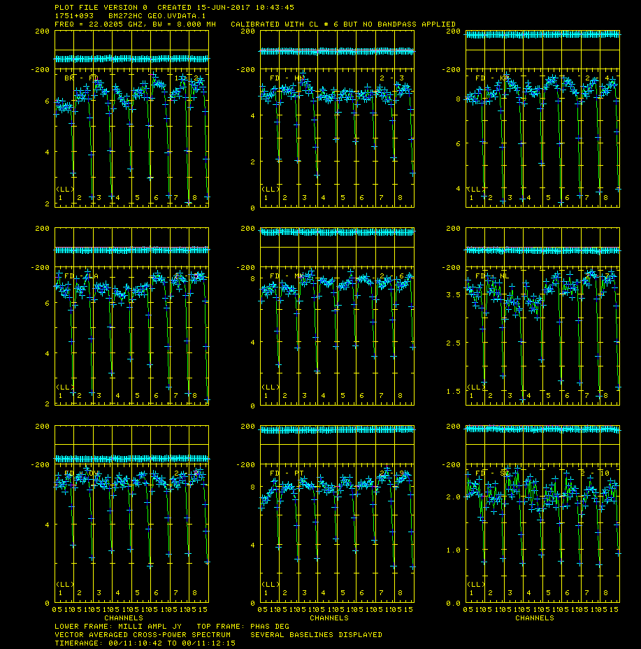
where the source and time range have been chosen to illustrate the differences clearly. | |||
After scrolling through the plots by pressing "B", or exiting with "D", generate plots with CL 6. | |||
# gainuse 6 | |||
# go | |||
Compare the phases to the same source when applying CL 6. As you can see in Figure 15b, the results look quite good after applying CL 6. | |||
{|style="margin: 0 auto;" | |||
| [[Image:POSSM_1751_093.CL5.png|380px|thumb|right|'''Figure 15a''' <br />POSSM plot showing source 1751+093 after applying CL table 5, which shows a slight phase slope across IF's.]] | |||
| [[Image:POSSM_1751_093.CL6.png|380px|thumb|right|'''Figure 15b''' <br />POSSM plot showing source 1751+093 after applying CL table 6, which shows improved flattened phases across all IF's.]] | |||
|} | |||
=== Solution transfer: Apply Delay Corrections === | |||
Now we transfer these solutions to the target dataset. | Now we transfer these solutions to the target dataset. | ||
This is where it gets a little complicated (although not much). Now we must apply the solutions to the data with the target in it | This is where it gets a little complicated (although not much). Now we must apply the solutions we derived above on the GEO data, to the original data with the target in it. The target data should have all the calibration done except the final fringe fit (CL table version 1). Then we can compare two versions/methods of this data reduction: images of the target data with previously final fringe fit done (CL table ver 2; non-DELZNed data), with the images of the target data to which we transferred the GEO solution (DELZNed data), and see which one is better. | ||
Use "imh" on the multi-source TARGET (SPLATed) data to see how many CL tables there are (two - if you followed this guide to the letter). We want to apply the [http://www.aips.nrao.edu/cgi-bin/ZXHLP2.PL?DELZN '''DELZN'''] solution to the CL table immediately before the final fringe fit we performed to that data. | |||
[ | |||
Apply the zenith delay correction with [http://www.aips.nrao.edu/cgi-bin/ZXHLP2.PL?CLCOR '''CLCOR''']. | Apply the zenith delay correction with [http://www.aips.nrao.edu/cgi-bin/ZXHLP2.PL?CLCOR '''CLCOR''']. | ||
| Line 675: | Line 812: | ||
# default clcor | # default clcor | ||
# getn 4 | # getn 4 | ||
# opco 'atmo'➜ read in a file of atmospheric and clock delay corrections and apply them to the given CL table. | # opco 'atmo' ➜ read in a file of atmospheric and clock delay corrections and apply them to the given CL table. | ||
# gainv 1; gainu | # gainv 1; gainu 0 ➜ input CL#1; generate a new CL table (CL 3). | ||
# infile 'FITS:delzn. | # infile 'FITS:delzn.clor ➜ file with corrections we created earlier with the GEO data. | ||
# inp | # inp | ||
# go | # go | ||
'''CLCOR''' will say it | '''CLCOR''' will say it has created CL table #3. Use this for further calibration, i.e. skip CL#2. | ||
=== Fringe Fit Data === | === Fringe Fit Data === | ||
Now, do the global fringe fit with [http://www.aips.nrao.edu/cgi-bin/ZXHLP2.PL?FRING '''FRING'''] on the DELZNed target data. This is where vput/vget come in handy, if you didn't do the vput, then repeat step previous FRING done on BM272HC.SPLAT.1 (Section 6.17), but change the gainuse parameter as shown below. | |||
# vnum 1; vget fring | # vnum 1; vget fring | ||
# gainu 3 | # gainu 3 | ||
# inp | # inp | ||
# go | # go | ||
Again, check the number of good and failed solutions: | |||
<pre> | |||
FRING1: Found 4498 good solutions | |||
FRING1: Failed on 42 solutions | |||
FRING1: Adjusting solutions to a common reference antenna | |||
</pre> | |||
You should get something similar but not necessarily exactly the same numbers of good and failed solutions. A small percentage of failed solutions are fine at this point. | |||
=== Apply Calibrations === | === Apply Calibrations === | ||
Apply calibration to tables with '''CLCAL'''. Again either use vnum/vget or repeat CLCAL step from above changing parameters as shown below. | Apply calibration to tables with [http://www.aips.nrao.edu/cgi-bin/ZXHLP2.PL?CLCAL '''CLCAL''']. Again, either use vnum/vget, or repeat CLCAL step from above (from Section 6.18), changing parameters as shown below. | ||
# vnum 1; vget clcal | # vnum 1; vget clcal | ||
# snver 2 | # snver 2 | ||
| Line 701: | Line 850: | ||
# gainu 4 | # gainu 4 | ||
# inp | # inp | ||
# go | # go | ||
=== Split the Data === | === Split the Data === | ||
Apply calibration to data with '''SPLIT'''. Here we can use tget because SPLIT has not been used since the last time we ran it on this data. Again repeat step | Apply calibration to data with [http://www.aips.nrao.edu/cgi-bin/ZXHLP2.PL?SPLIT '''SPLIT''']. Here we can use tget because SPLIT has not been used since the last time we ran it on this data. Again repeat step 6.19 if you can't do this. | ||
# tget split | # tget split | ||
# gainu 4 | # gainu 4 ➜ apply CL#4 to the data | ||
# outcl 'delzn' | # outcl 'delzn' | ||
# inp | # inp | ||
# go | # go | ||
=== Image J2007+4029 === | === Image J2007+4029 === | ||
Image J2007+4029 with '''IMAGR'''. | Image J2007+4029 with [http://www.aips.nrao.edu/cgi-bin/ZXHLP2.PL?IMAGR '''IMAGR''']. | ||
# tget imagr | # tget imagr | ||
# getn 17 | |||
# cell 3e-5 | # cell 3e-5 | ||
# imsi 512 | # imsi 512 | ||
| Line 729: | Line 882: | ||
# go | # go | ||
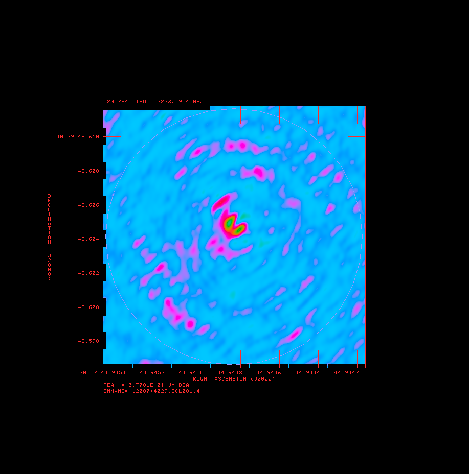
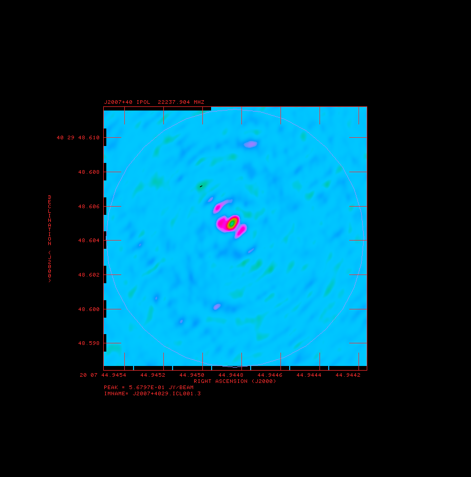
Use the correct catalog number for J2007+4029 DELZN version. It was 17 on my disk. Then run IMAGR and compare the new image to the one made without the correction (Figure 16a). | |||
{|style="margin: 0 auto;" | |||
| [[Image:J2007_4029_IMAGR_UnCorr.png|380px|thumb|right|'''Figure 16a''' <br />IMAGR screenshot showing source J2007+4029 before applying DELZN delay corrections and before applying fringe fitted calibrations.]] | |||
| [[Image:J2007_4029_IMAGR_Corr.png|380px|thumb|right|'''Figure 16b''' <br />IMAGR screenshot showing source J2007+4029 after applying DELZN delay corrections and applying fringe fitted calibrations. Peak flux has increased and position has been corrected.]] | |||
|} | |||
As you can see, the image after the correction (Figure 16b) has a lower noise level and a source with a higher peak. Bad phases spread the flux around the image and make the noise level higher and source flux lower as well as shifting the position of the source. | |||
</div> | |||
<!-- | <!-- | ||
--Original: Mioduszewski, Amy <br /> | --Original: Mioduszewski, Amy <br /> | ||
--Wiki: Salcido, Jose <br /> | --Wiki: Salcido, Jose & Kapinska, Anna <br /> | ||
--> | --> | ||
Latest revision as of 20:38, 13 May 2022
Overview
A good resource for reducing basic VLBI data in AIPS can be found in Appendix C of the AIPS Cookbook. Chapter 9:Reducing VLBI Data in AIPS of the AIPS Cookbook contains much more detail, but is best used as a reference. Details on the geodetic like calibration to improve phase referencing and astrometry can be found in AIPS Memo 110: Strategy for Removing Tropospheric and Clock Errors using DELZN. In short, to obtain precise positions and good image quality with phase referencing in VLBI, two things are needed; a close calibrator to the target source to minimize atmospheric differences between the target and calibrator and a good correlator model. The VLBA correlator uses a model for the troposphere computed from seasonal models as well as the best estimates of the clocks, positions of each antenna, and earth orientation parameters. These major sources of error produce a systematic phase difference between the calibrator and target which limits the target positional accuracy and image quality. The troposphere model error, however, can be estimated by observing about ten calibrators over the sky over a 30-minute period, and then calculating the erroneous delay. So with this tutorial you will:
- Calibrate the regular data all the way through imaging.
- Calibrate the geodetic style data through instrumental delay removal.
- Compute the Multi-band Delay (MBD). The MBD is a function of a variable clock delay, and a troposphere term (zenith path delay) which has a well-defined function of elevation (called a mapping function), times an unknown constant.
- Use the AIPS task DELZN to fit the MBD and calculate the clock and zenith path delay error.
- Apply these corrections to the dataset that includes the target.
- Image the target and see an improvement over not doing the geodetic calibration.
This guide only gives the important inputs to each task. The other inputs should be left at their defaults. An easy way to set all the inputs to the default in a task is to type "default taskname".
AIPS
For a comprehensive overview of AIPS see the AIPS COOKBOOK, especially Chapter 3:Basic AIPS Utilities and Chapter 12:AIPS for the More Sophisticated Userfor the basics. Chapter 9:Reducing VLBI Data in AIPS is the chapter explaining VLBI data reduction, but it is rather overwhelming so Appendix C:A Step-by-Step Recipe for VLBA Data Calibration in AIPS is recommended as a first step. However, below I summarize some useful commands (in parenthesis are the short form of the command):
- getname (getn) catalog #: get the name of catalog # and fill in INNAME, INCLASS and INSEQ. Other similar: geton (get outname); get2n (get in2name); get3n (getin3name) etc..
- input (inp) taskname: show the inputs of taskname.
- tget taskname: get a task and fill in the inputs of the last time the task was run, one of the most useful commands in AIPS.
- ucat (uc): list uvdata catalog.
- mcat (mc): list map catalog.
- pca: list all catalogs.
- tvlod (tvlo): load a map onto the TV.
- tvinit (tvin): initialize and clear TV.
- imhead (imh): Print the file header (this can be used on both uv data and images despite the name). This will list informative things like the date of observation and the number and types of tables attached to the data.
Getting the Data
To obtain the data, right click on these file names below and select "Save Link As..." . Put the data into your $FITS area, which should be an AIPS area that is automatically set up when you install AIPS.
- BM272HC.fits (12 GB): Data containing target and calibrators.
- BM272HC_geodetic.fits (0.3 GB): Data containing geodetic block. These are observations of many calibrators around the sky.
If that doesn't work you can also ftp the data using anonymous ftp:
- ftp ftp.aoc.nrao.edu
- login as anonymous
- cd pub/SIW
- mget *.fits
The geodetic blocks are in a different file from the target because they have very different frequency setups. The geodetic block is required to have widely spaced frequencies with a single polarization in order to measure the multi-band delay (MBD). The target dataset is dual polarization (important since the source is circularly polarized) and frequencies that are continuous. MAKE SURE YOU ARE RUNNING THE CORRECT TASK ON THE CORRECT DATASET!
About the Data
This is an observation of water masers in star-forming region IRAS 00420+5530 and involves phase referencing. The sources in the the BM272HC.fits dataset are as follows:
- AFGL2591 - phase calibrator/target (maser source for which the position is desired)
- J2007+4029, 20330+40003, 20327+40396, 20324+40574 - calibrators that are phase referenced to AFGL2591 (note that only J2007+4029 and 20330+40003 are detected).
- 3C345A, 3C454.3A - Bright, well known quasars, used as fringe finders and bandpass calibrators
The BM272HC_geodetic.fits dataset contains numerous sources (all known quasars) observed all over the sky but the specifics are unimportant.
This data was published by Rygl et. al
Starting AIPS and Loading the Data
Starting AIPS
Start AIPS by typing aips or possibly aips tv=local:0.0 in a terminal window. Depending on your AIPS installation, you might be prompted to pick a printer, then you will be asked for an AIPS number, if you are not sharing disks with anyone pick any number other than 1. Remember that number because the data you load and work on will be under that number. It would be best for this tutorial for you to use a clean AIPS number, in other words, an AIPS number that you have not used for anything else and has no data loaded into it.
Loading Data Into AIPS
Load the data with FITLD. Note that I am forcing an outname, outclass and outseq, we are doing it here so it will be easy to take about specific files.
- First load the target and calibrators
- default fitld
- clint 0.25 ➜ set CL table interval to 15 seconds.
- datain 'FITS:BM272HC.fits ➜ Two things to note: 1) this assumes that the data is in the $FITS directory, you can use a full directory path (e.g., datain '/home/mydata/BM272HC.fits) or another environmental variable if the data is elsewhere; 2) The lack of a close ' is not a typo, you must leave off the closing ' or AIPS will capitalize the everything within the ' ' and you will get an error because FITLD will not be able to find the data.
- outname 'bm272hc'
- outclass 'uvdata'
- outseq 1
- outdisk 1
- inp ➜ check the inputs
- go
- Now load the geodetic block, this is a good place to talk about global inputs. Once you set an input it will stay set for all tasks until you change it. So notice below we do not set clint, outclass, outseq or outdisk, this is because we want the same values as above and they are already set.
- datain 'FITS:BM272HC_geodetic.fits ➜ again remember to leave off the close '.
- outname 'BM272HC GEO'
- go
- Lets look at our uv data catalog
- uc
You should get something that looks similar to (with a different Usid and Last access):
AIPS 1: Catalog on disk  1
AIPS 1:   Cat  Usid Mapname      Class   Seq  Pt    Last access     Stat
AIPS 1:     1  1709 BM272HC     .UVDATA.    1 UV 07-APR-17 15:35:37
AIPS 1:     2  1709 BM272HC GEO .UVDATA.    1 UV 07-APR-17 15:36:29
Note each file has a catalog number (Cat), BM272HC.UVDATA.1 is catalog number 1 and BM272HC GEO.UVDATA.1 is catalog number 2. These catalog numbers can be, and usually are, used to fill in IN and OUTNAMES etc., using getn, geton etc..
Reducing the phase referencing data (BM272HC.UVDATA.1)
Preliminary Data Evaluation
Look at the structure of the data with LISTR. This will give you a listing of the scans as well as the source and frequency structure in the observation.
- default listr
- getn BM272HC.UVDATA.1 file; in other words getn 1
- optype 'scan'
- docrt 1
- inp
- go
Data Reduction Procedure for BM272HC
Load in the VLBA data reduction procedures: see EXPLAIN VLBAUTIL for full description of procedures.
Procedures are run by just typing their name, rather than using "go".
- run vlbautil
If you get a BLEW CORE or other similar error message, you have filled your procedure memory (VLBAUTIL is very large and loading it three times will do this). To fix it type "restore 0" then reload VLBAUTIL
Calibrate Ionospheric Delay
Fix ionosphere contribution to the dispersive delay by running VLBATECR.
- default vlbatecr
- getn 1
- inp
- vlbatecr ➜ to run VLBATECR
Fix Earth Orientation Parameters
Fix earth orientation parameters by running VLBAEOPS.
- default vlbaeops
- getn 1
- inp
- vlbaeops
Apply Digital Sampling Correction to VLBA data
Correct sampler threshold errors from correlator by running VLBACCOR.
- default vlbaccor
- getn 1
- inp
- vlbaccor
Plot Cross Power Spectrum
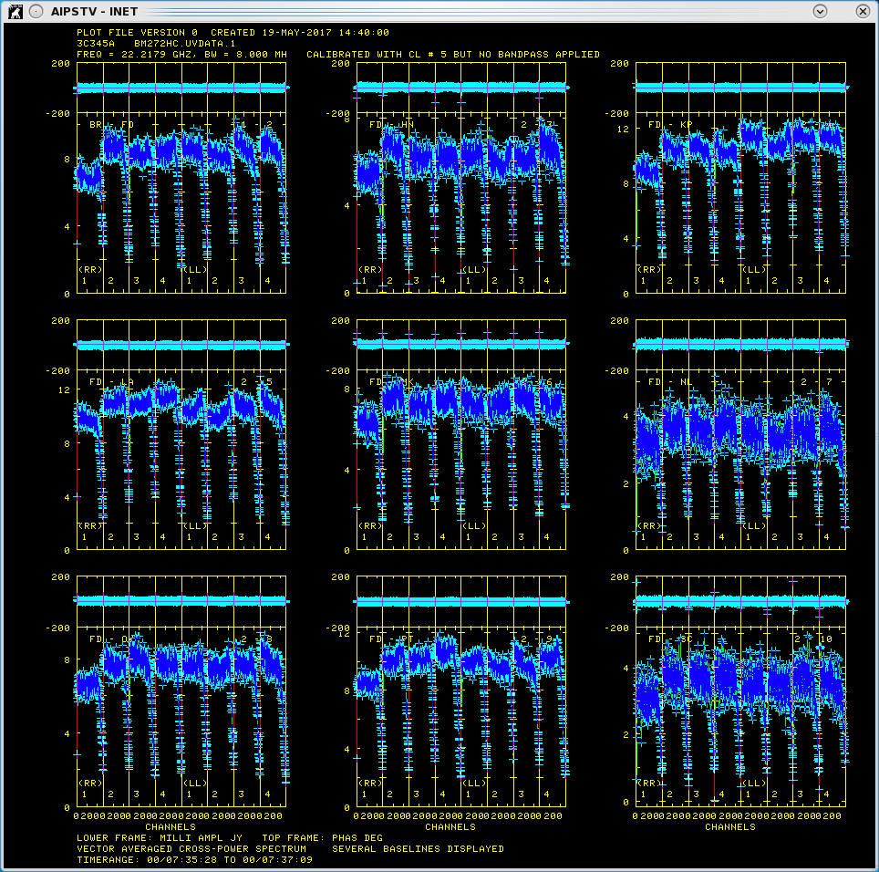
Plot of amplitudes (bottom) and phases (top) for source 3C345A .
Now lets take a look at the fringe finders by running VLBACRPL. VLBACRPL runs POSSM and displays the spectrum of each baseline (to Fort Davis (antenna 2)), with the amplitude on the bottom and the phases on the top.
- default vlbacrpl
- getn 1
- stokes 'half'
- refant 2
- gainuse 0
- solint -1
- dotv 1
- source '3C345A' '3C454.3A'
- inp
- vlbacrpl
As you can see from Figure 1, 3C345A has very strong fringes. So we will use it as the calibrator to set the instrumental delays. Also look at your terminal for instructions on how to control POSSM:
POSSM1: Waiting 30 seconds:
POSSM1:    Hit TV button A to pause indefinitely.  Hit button
POSSM1:    B or C to continue sooner, button D to stop plotting
So hit A if you want to look at a plot longer than the 30 seconds, B or C to go to the next plot, D to exit.
Determine Delay Corrections
Find and remove instrumental delay by running VLBAMPCL.
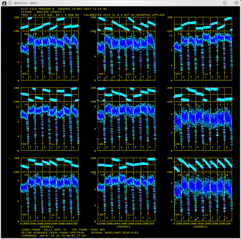
Plots for source 3C345A which show the amplitude (bottom panel) and corrected phases (top panel), for each IF in both polarizations.
- default vlbampcl
- getn 1
- calsour '3C345A' ' ➜ strongest source.
- timer 0 07 35 28 0 07 37 09 ➜ scan with good fringes we found in POSSM plots.
- refant 2 ➜ choose reference antenna from in the middle of array, FD (antenna 2) is a good choice.
- gainu 0 ➜ apply highest CL table.
- inp
- vlbampcl
At this point you should check on the calibration:
- First check you have no failed solutions. At the end of the FRING run it should tell you how many "good" and "failed" solutions it has found. The output from FRING will look something like this:
FRING1: Writing SN table    2
FRING1: Time=   0/ 07 36 19, Polarization = 1
FRING1: Time=   0/ 07 36 19, Polarization = 2
FRING1: Found       80 good solutions
FRING1: Adjusting solutions to a common reference antenna
For this step there must be no failed solutions. Failed solutions in this step means that whichever antenna the failed solution was on is deleted from your data. For this data, because there are 10 antennas, 2 polarizations and 4 spectral windows (IFs), there should be "80 good solutions".
- check solutions in POSSM, the jumps in phase between the IFs should be gone. The phases may also be flattened.
- tget possm ➜ to "get" all the inputs from the last run (it was run when we ran the procedure VLBACRPL).
- gainu 5
- inp
- go
As you can see from Figure 2, the phases for 3C345A have been flattened and the phase jumps between the IFs are gone. For other sources farther away in time the phases may be different from 0 but there will still be no phase jumps.
Create BP Table and Calibrate Bandpass Shape
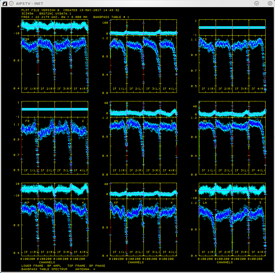
Plot of bandpass for source 3C345A .
Calibrate bandpass shape with VLBABPSS.
- default vlbabpss
- getn 1
- calsour '3C345A' '3C454.3A' ➜ use both very strong sources as bandpass calibrators.
- refant 2
- inp
- vlbabpss
Now check the bandpass solutions with POSSM.
- tget possm
- baseline=0
- aparm=0
- aparm(8)=2
- aparm(9)=1
- bpver=1; doband=1
- go
Figure 3 shows the plots generated by POSSM. The solutions should look like a reasonable fit of the bandpass shape.
Apply Amplitude Corrections
Perform amplitude calibration by running VLBAAMP.
- default vlbaamp
- getn 1
- inp
- vlbaamp
Examine Amplitude Calibration
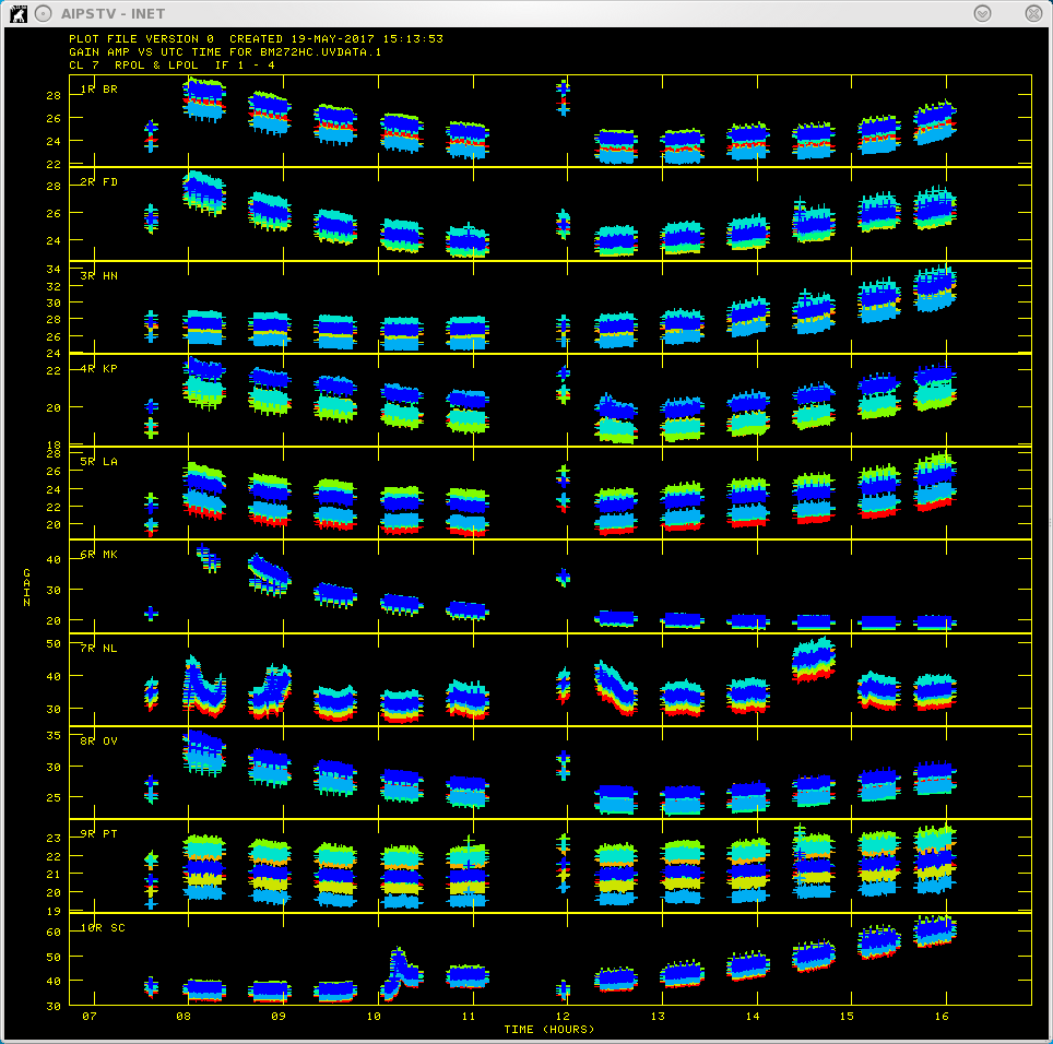
Plot of amplitude gains vs. time with the different colors representing the different IF polarizations.
Examine amplitude calibration by running SNPLT.
- default snplt
- getn 1
- dotv 1
- inext 'cl'
- invers 0
- opty 'amp' ➜ Plot amplitudes.
- nplots 10
- opco 'alsi' ➜ Plot all IFs and Stokes.
- do3col 1 ➜ Use 3-color symbols.
- inp
- tvin ➜ tvinitialize clears the tv before plotting. Otherwise you will get a mess as the table is plotted over the bandpass plot from before.
- go
Figure 4 shows the amplitude gains change over time as the sources rise and set, with higher gains at lower elevations. Because 3C345 and 3C454.3 are so strong, they will increase the gains. The different IFs and polarizations (RR and LL in this case) are shown as different colors.
Correct Phases for Parallactic Angles
Correct phases for parallactic angle effects with VLBAPANG.
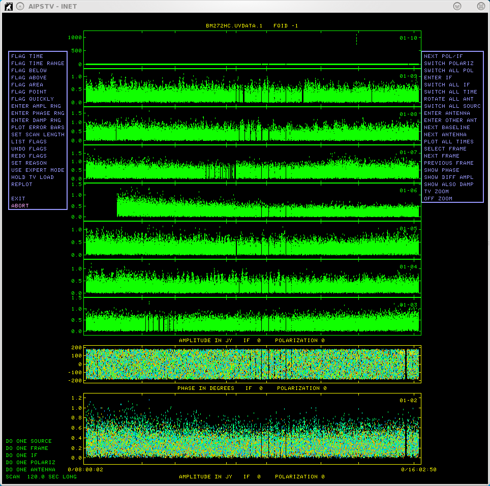
EDITR plot showing a high data point for baselines 01-10 that we will need to flag.
- default vlbapang
- getn 1
- inp
- vlbapang
Manually Edit Data
EDITR plot showing the cutoff area for the FLAG ABOVE option. Every data point above the cutoff line will be flagged.
A "REPLOT" of baseline 01-10, after flagging of the high data point and re-scaling.
Edit the data using EDITR on each source separately.
- default editr
- getn 1
- docal 1; gainuse 0 ➜ calibrate data with highest CL table.
- crowded 1 ➜ to plot all polarization and IFs on top of each other.
- do3col 1
- doband 1
- bpver 1
- flagver 1
- outfgver 1
- antuse 1 2 3 4 5 6 7 8 9 10 ➜ to plot all the baselines to one antenna at the same time.
- source 'AFGL2591'' ➜ run on one source at a time
- inp
- go
Again look in your terminal window for intructions:
EDITR1: Press buttons A, B, or C to choose an operation
EDITR1: Press button D for on-line help
Note that the data looks great but there are a few high points we'll want to flag. The data we want to flag is found on baseline 01-10 as seen in Figure 5. Click "NEXT BASELINE" found on the menu to the right and press "B" until baseline 01-10 is plotted in the edit window at the bottom of the display . We will now flag the high points with flagging options found on the left menu. Click "FLAG ABOVE" and hit B. Your mouse cursor should shift to the edit window. In the terminal window you will now see instructions for FLAG ABOVE:
EDITR1: Hit buttons A or B to flag high fluxes and continue
EDITR1: Hit button C to flag high fluxes and return to menu
EDITR1: Hit button D to return to menu with no more flagging
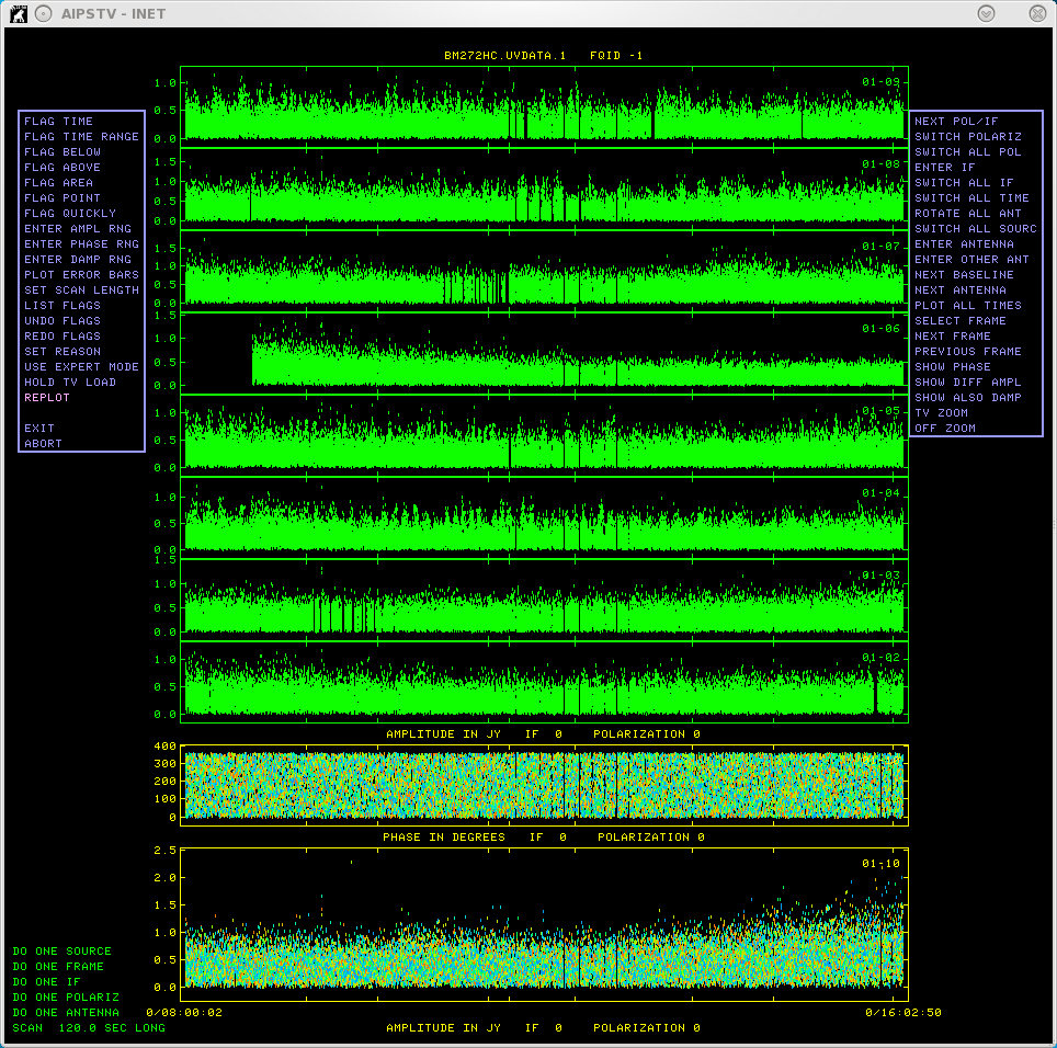
Choose where to place your cutoff line as seen in Figure 6. Every data point above this line will be flagged. Press "C" to flag the high fluxes and return to the menu. The data points should now be highlighted white. To view the results of the flagging, we can generate a new plot by clicking "REPLOT" and pressing B. The plot will update without the high data points as seen in Figure 7. There are two more baselines with similar problems. Click NEXT ANTENNA and button B repeatedly to examine all of the data. When bad points are found, click NEXT BASELINE and button B until the offending baseline appears in the edit window, and then click FLAG ABOVE with button B to remove the bad samples. Finally, on the left menu, click on "EXIT" then press B. This will write the flags to a new flagging table (FG) which we can later apply to the data.
Now plot the other sources and inspect.
- 20330+40003:
- source '20330+40003''
- go
- J2007+4029:
- source 'J2007+4029''
- go
EDITR plots both amplitudes and phases, so this is a good way to just look at your data. If you plot the phases on all the baselines, note that you can see coherent phases on J2007+4029, but not the other two sources. AFGL2591 has strong masers that fringe, but EDITR is plotting all the channels averaged.
Backing up Your Calibration
We will want to save the calibration up to this point with TASAV. TASAV makes a new file with all your calibration tables, this is very useful because it contains everything you need to recalibrate your data in a very compact and portable form. It is also a good idea to do this before you do anything you are unsure about or will change important tables (AN, SU) in ways that are hard to change them back. In the next step we are changing the SU table.
- default tasav
- getn 1
- outdisk 1
- inp
- go
Lets look at our catalog again:
- uc
You should get something that look similar to:
AIPS 1: Catalog on disk  1
AIPS 1:   Cat  Usid Mapname      Class   Seq  Pt    Last access     Stat
AIPS 1:     1  1099 BM272HC     .UVDATA.    1 UV 07-APR-17 16:19:59
AIPS 1:     2  1099 BM272HC GEO .UVDATA.    1 UV 07-APR-17 15:36:29
AIPS 1:     3  1099 BM272HC     .TASAV .    1 UV 07-APR-17 16:19:59
Note that you now have a third catalog entry which TASAV automtically named BM272HC.TASAV.1. This uv data file has 1 visibility and all the tables attached to BM272HC.UVDATA.1. Lets look at the TASAVed file.:
- getn 3
- imh
You should get something that looks like:
AIPS 1: Image=MULTI     (UV)         Filename=BM272HC     .TASAV .   1
AIPS 1: Telescope=VLBA               Receiver=
AIPS 1: Observer=BM272               User #= 1099
AIPS 1: Observ. date=13-MAY-2009     Map date=14-APR-2017
AIPS 1: # visibilities         1     Sort order  TB
AIPS 1: Rand axes: UU-L-SIN  VV-L-SIN  WW-L-SIN  TIME1  SUBARRAY
AIPS 1:            SOURCE  FREQSEL  INTTIM  GATEID  CORR-ID  ANTENNA1
AIPS 1:            ANTENNA2
AIPS 1: ----------------------------------------------------------------
AIPS 1: Type    Pixels   Coord value     at Pixel     Coord incr   Rotat
AIPS 1: COMPLEX      3   1.0000000E+00       1.00  1.0000000E+00    0.00
AIPS 1: STOKES       2  -1.0000000E+00       1.00 -1.0000000E+00    0.00
AIPS 1: FREQ       256   2.2217920E+10       1.00  3.1250000E+04    0.00
AIPS 1: IF           4   1.0000000E+00       1.00  1.0000000E+00    0.00
AIPS 1: RA           1    00 00 00.000       1.00       0.000000    0.00
AIPS 1: DEC          1    00 00 00.000       1.00       0.000000    0.00
AIPS 1: ----------------------------------------------------------------
AIPS 1: Coordinate equinox 2000.00
AIPS 1: Maximum version number of extension files of type HI is   1
AIPS 1: Maximum version number of extension files of type FQ is   1
AIPS 1: Maximum version number of extension files of type CT is   1
AIPS 1: Maximum version number of extension files of type OB is   1
AIPS 1: Maximum version number of extension files of type AN is   1
AIPS 1: Maximum version number of extension files of type CL is   8
AIPS 1: Maximum version number of extension files of type CQ is   1
AIPS 1: Maximum version number of extension files of type GC is   1
AIPS 1: Maximum version number of extension files of type IM is   1
AIPS 1: Maximum version number of extension files of type MC is   1
AIPS 1: Maximum version number of extension files of type PC is   1
AIPS 1: Maximum version number of extension files of type SU is   1
AIPS 1: Maximum version number of extension files of type TY is   1
AIPS 1: Maximum version number of extension files of type WX is   1
AIPS 1: Maximum version number of extension files of type SN is   4
AIPS 1: Maximum version number of extension files of type BP is   1
AIPS 1: Maximum version number of extension files of type FG is   1
Note that there are 8 calibration (CL) tables and 4 solution (SN) tables. As well as numerous other tables with information about your data (history (HI), frequency (FQ), antenna (AN), system temperature (TY), bandpass (BP), flag (FG)...).
Apply Correction to CL Table
We will now shift the position of AFGL2591 with CLCOR. The observed/correlated position of AFGL2591 was quite wrong and shifting a large distance in the image plane is imprecise, therefore it is important to shift the uv-data with either CLCOR or UVFIX. Normally you would reduce and image the data to find the shift.
- default clcor
- getn 1
- sour 'AFGL2591' '
- gainver 8
- gainuse 9
- opcode 'antp'
- clcorprm(5)= 0.009 ➜ Correction in RA direction in seconds of arc.
- clcorprm(6)=-0.129 ➜ Correction in Dec direction in seconds of arc.
- inp
- go
Note: If you do something wrong in this step, just doing the same shift in reverse will not undo the shift to astrometric accuracy due to the complications of precession. This is why we did the TASAV step. To undo the shift, delete the CL table that was created by CLCOR and the SU table using EXTDEST. Then copy the SU table from the TASAVed file with TACOP.
Apply Calibrations
Apply all calibration up to this point and copy out IF#3 with SPLAT.
The masers are in the 3rd IF and we will be fringe fitting on that maser so we should get rid of the other IFs. We could have gotten rid of the other 3 IFs earlier, but I kept them around for two reasons, 1) I wanted you to see what more than one IF looked like in displays and editing, since most of the data you will receive will be more than one IF; and 2) it is a good idea to apply the calibration after the position shift, but before global fringe fitting and the zenith delay correction.
- default splat
- getn 1
- bif 3; eif 3
- docal 1
- gainu 9
- doband 1
- bpver 1
- inp
- go
For the next 4 steps you will be running the AIPS tasks on the dataset out of SPLAT. Lets look at the catalog again.
- uc
AIPS 1: Catalog on disk  1
AIPS 1:   Cat  Usid Mapname      Class   Seq  Pt    Last access     Stat
AIPS 1:     1  1099 BM272HC     .UVDATA.    1 UV 07-APR-17 16:19:59
AIPS 1:     2  1099 BM272HC GEO .UVDATA.    1 UV 07-APR-17 15:36:29
AIPS 1:     3  1099 BM272HC     .TASAV .    1 UV 07-APR-17 16:19:59
AIPS 1:     4  1099 BM272HC     .SPLAT .    1 UV 07-APR-17 17:46:29
BM272HC.SPLAT.1 is catalog number 4. Also if you see a gap in the catalog numbers, say BM272HC.SPLAT.1 was catalog number 5, then type recat, and it will remove any gaps.
Plot Power Spectra
A plot showing the maser in channel 145.
Select channel for global fringe fit with POSSM.
- tget possm
- getn 4
- sour 'AFGL2591' '
- base 2 0
- gainu 0
- solint -1
- doband -1
- docal -1
- aparm 0, 1, 0, 0, -180, 180, 0, 0, 1
- dotv 1
- nplots 1
- bchan 100; echan 180
- inp
- go
We really only need to look at one spectrum for this, so you can hit "D" right away or go through a few plots to see how the spectrum changes a bit from baseline to baseline.
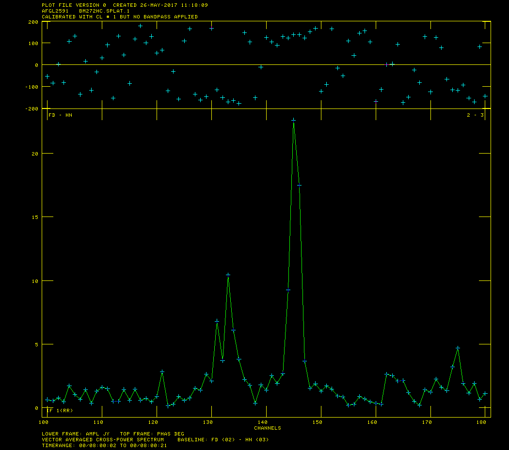
Figure 8 shows that the maser is strongest in channel 145 on a baseline FD-HN.
Fringe Fit the Data
Perform a global fringe fit with FRING. The following steps through imaging are not strictly necessary since we will have to redo them once the geodetic calibration is done, but is an excellent way to check that the calibration up to this point is correct.
- default fring
- getn 4
- calsour 'AFGL2591' ' ➜ do a global fringe fit on maser.
- bchan 145;echan 145
- refant 2
- search 2 9 5 4 1 3 7 8 ➜ list of antennas to search if a solution is hard to find.
- aparm(9) 1 ➜ do exhaustive baseline search.
- docal 1; gainu 0
- inp
- go
You should look at the number of good and failed solutions:
FRING1: Found     4506 good solutions
FRING1: Failed on       34 solutions
FRING1: Adjusting solutions to a common reference antenna
You should get something similar but not necessarily exactly the same numbers of good and failed solutions. A small percentage of failed solutions are fine at this point.
Hint: We will have to do this exact same step after doing the zenith delay calibration so it is helpful to save the inputs to FRING. This can be done with vnum and vput.
- vnum 1; vput fring
Apply FRING solutions from AFGL2591 to Calibrators
Note that this is "phase referencing", you are getting phases on one source and applying them to another, nearby source. However the way we are doing it here is a little backwards, in most situations your target it too faint to use in FRING and you run FRING on one of the calibrators and apply those phases to your target. Here we are using the target maser in FRING because it is stronger and applying it to the calibrators because we care about positions. In this case any shift in the position of the calibrators will indicate that AFGL2591 has moved. Interpolate the fringe solutions with CLCAL.
- default clcal
- getn 4
- gainv 1 ➜ CL table with all the calibration.
- gainu 2 ➜ CL table to write next step of calibration in.
- snver 1 ➜ contains final fringe fit.
- interpol '2PT' ➜ use 2PT interpolation.
- refant 2
- sour 'AFGL2591' '20330+40003' 'J2007+4029' ➜ sources to which to apply calibration.
- calsour 'AFGL2591' ' ➜ phase calibrator, phases will be applied from AFGL2591 to itself, 20330+40003 and J2007+4029.
- inp
- go
This is another spot where vnum and vput will be useful:
- vnum 1; vput clcal
Apply Calibration and SPLIT the Data
Apply calibration and make single source data sets with SPLIT. I like to work with single source files, it's less confusing, especially when self-caling and imaging.
- default split
- getn 4
- freqid 0
- docal 1; gainu 2 ➜ apply calibration; from CL#2.
- sour 'AFGL2591' '20330+40003' 'J2007+4029' ➜ split out target and phase calibrators.
- inp
- go
This will produce three files named sourcename.SPLIT.1, again type uc to look at the catalog.
AIPS 1: Catalog on disk  1
AIPS 1:   Cat  Usid Mapname      Class   Seq  Pt    Last access     Stat
AIPS 1:     1  1099 BM272HC     .UVDATA.    1 UV 07-APR-17 20:18:29
AIPS 1:     2  1099 BM272HC GEO .UVDATA.    1 UV 07-APR-17 15:36:29
AIPS 1:     3  1099 BM272HC     .TASAV .    1 UV 07-APR-17 16:22:12
AIPS 1:     4  1099 BM272HC     .SPLAT .    1 UV 07-APR-17 20:18:29
AIPS 1:     5  1099 AFGL2591    .SPLIT .    1 UV 07-APR-17 20:18:11
AIPS 1:     6  1099 J2007+4029  .SPLIT .    1 UV 07-APR-17 20:18:17
AIPS 1:     7  1099 20330+40003 .SPLIT .    1 UV 07-APR-17 20:18:29
Create Image of AFGL 2591
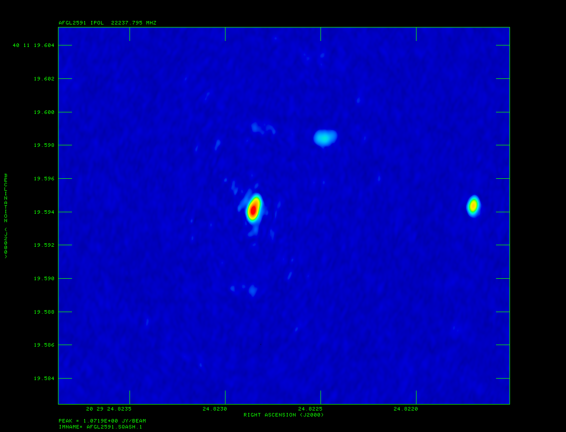
A radio image of the maser AFGL 2591.
Image AFGL 2591 with IMAGR.
- default imagr
- getn 5
- bchan 125; echan 150; nchav 1; ➜ image channels 125-150.
- cell 3e-5; imsi 1024 ➜ cell size of 0.03 mas; image size of 1024x1024.
- dotv 1; niter 1000 ➜ do interactive clean; with 1000 iterations.
- im2parm 10 6 9 0.5 ➜ autoboxing, only do 10 boxes per major cycle; find islands with > 6*rms; box is accepted if peak > 9*rms; box is accepted if its peak brightness is >0.5*max residual.
- inp
- go
HINT: The first few channels will not have any masers, just hit "STOP CLEANING" (and "A" to select, again look at the terminal for instructions) until you see some emission. Hit TVPSEUDO (and "A"), then "D" immediately to get color rather than grey scale. If you want to clean interactively, then click CONTINUE CLEAN (and "A"); if you want to add boxes use REBOX ("A"); when you are happy with the cleaning you can go to the next channel by clicking STOP CLEANING ("A"). You can turn off interactive clean by clicking TURN OFF DOTV ("A"). However, the appropriate stopping point in each channel varies both in terms of number of iterations and lowest believable flux, so you should interact with each channel patiently. Once IMAGR is done, you can do a mcat (mc for short) to look at the maps in your catalog:
- mc
AIPS 1: Catalog on disk  1
AIPS 1:   Cat  Usid Mapname      Class   Seq  Pt    Last access     Stat
AIPS 1:     8  1099 AFGL2591    .IBM001.    1 MA 14-APR-17 10:58:28
AIPS 1:     9  1099 AFGL2591    .ICL001.    1 MA 14-APR-17 10:58:28
Note that you have made two files, a "dirty beam" (the IBM001 file) and a cleaned map (ICL001).
Look at cube with AFGL2591 TVMOVIE (getn 9; tvmovie). Then collapse the cube with SQASH
- default sqash
- getn 9
- bdrop 3
- dparm 1 0
- go
SQASH will produce another map in your catalog:
- mc
AIPS 1: Catalog on disk  1
AIPS 1:   Cat  Usid Mapname      Class   Seq  Pt    Last access     Stat
AIPS 1:     8  1099 AFGL2591    .IBM001.    1 MA 14-APR-17 10:58:28
AIPS 1:     9  1099 AFGL2591    .ICL001.    1 MA 14-APR-17 11:02:50
AIPS 1:    10  1099 AFGL2591    .SQASH .    1 MA 14-APR-17 11:02:50
To look at it use TVLOD (getn 10; tvin; tvlo). Use TVPSEUDO to put it into color (tvps). You can use your mouse to manipulate the colors, looking again at your terminal for instructions. Hit "D" once it looks the way you want. Figure 9 shows the SQASH result.
Create More Images
Image J2007+4029 and/or 20330+40003 with IMAGR to make sure phase referencing worked.
- default imagr
- getn 6 or 7
- bchan 0; echan 0; nchav 256; ➜ average all channels.
- cell 3e-5;imsi 2048 ➜ larger image size because sources might not be at center of field.
- im2parm 10 6 9 0.5 ➜ autoboxing again
- dotv 1; niter 1000 ➜ do interactive clean; with 1000 iterations.
- inp
- go
Here I would check that the autobox looks OK (It should just be around the the obvious emission) and then hit TURN OFF DOTV ("A"). Figure 10 shows the end result of running IMAGR on J2007+4029 (getn 6). To image 20330+40003 you will need to set IMSIZE to 8192. The assumed coordinate for this source was not entirely correct.
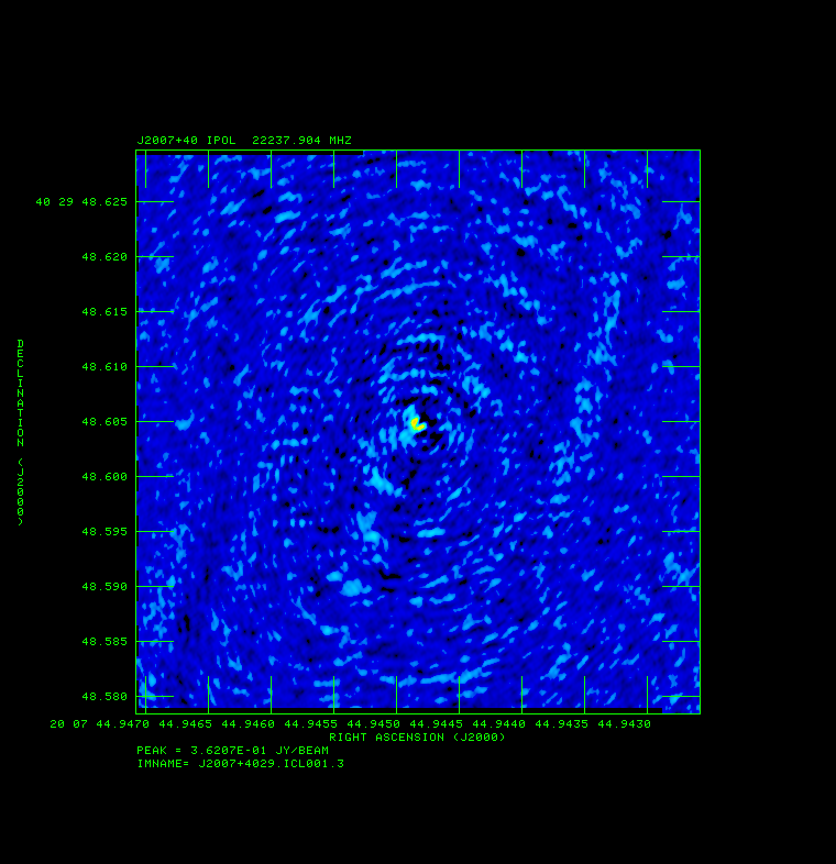
A radio image of J2007+4029.
Now do an mcat to see the maps we have created:
- mc
AIPS 1: Catalog on disk  1
AIPS 1:   Cat  Usid Mapname      Class   Seq  Pt    Last access     Stat
AIPS 1:     8  1099 AFGL2591    .IBM001.    1 MA 14-APR-17 10:58:28
AIPS 1:     9  1099 AFGL2591    .ICL001.    1 MA 14-APR-17 11:02:50
AIPS 1:    10  1099 AFGL2591    .SQASH .    1 MA 14-APR-17 11:04:16
AIPS 1:    11  1099 J2007+4029  .IBM001.    1 MA 14-APR-17 11:14:05
AIPS 1:    12  1099 J2007+4029  .ICL001.    1 MA 14-APR-17 11:14:05
Then getn 12; tvin; tvlo; tvps.
Reducing geodetic-style data (BM272HC GEO.UVDATA.1)
The following contains instructions for the geodetic-like calibration to improve astrometry (and phase referencing).
We start with the same steps 4-8 as above on the geodetic data. Its name should be something like "BM272HC GEO.UVDATA.1" if you followed the naming I suggested in the FITLD step above.
Calibrate Ionospheric Delay
Fix ionosphere contribution to the dispersive delay by running VLBATECR.
- default vlbatecr
- getn 2
- inp
- vlbatecr ➜ to run VLBATECR
Fix Earth Orientation Parameters
Fix earth orientation parameters by running VLBAEOPS.
- default vlbaeops
- getn 2
- inp
- vlbaeops
Apply Digital Sampling Correction to VLBA data
Correct sampler threshold errors from correlator by running VLBACCOR.
- default vlbaccor
- getn 2
- inp
- vlbaccor
Plot Cross Power Spectrum
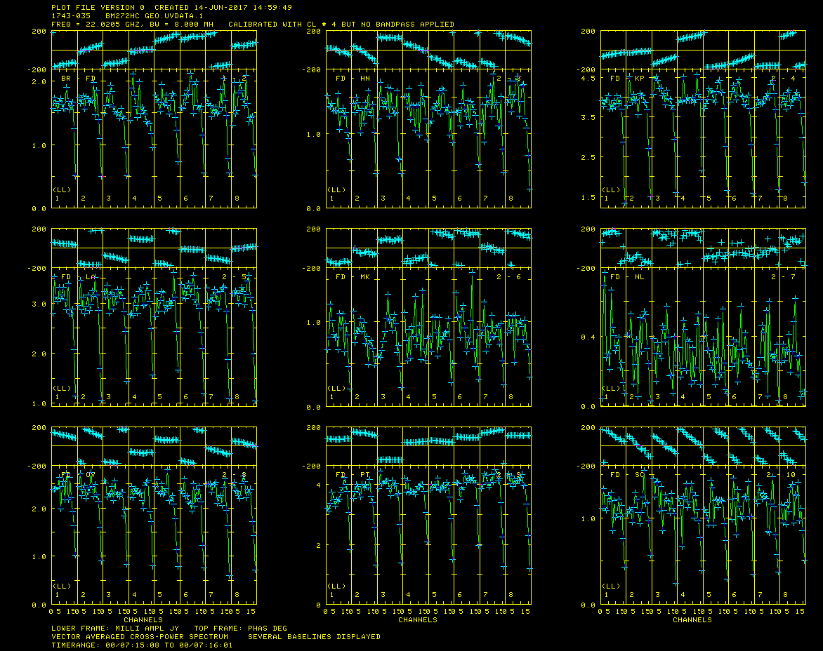
Cross power spectrum plot of 1743-035 showing strong fringes.
Now find a scan that has good fringes on all the baselines by running VLBACRPL. VLBACRPL runs POSSM and displays the spectrum of each baseline (to Fort Davis (antenna 2)), with the amplitude on the bottom and the phases on the top.
- default vlbacrpl
- getn 2
- stokes 'half'
- refant 2
- gainuse 4
- solint -1
- dotv 1
- inp
- vlbacrpl
Hit "B" a few times to go through the scans. Although there are several sources/scans to choose from, I choose 1743-035, which has strong fringes on all baselines as seen in Figure 11.
Determine Delay Corrections
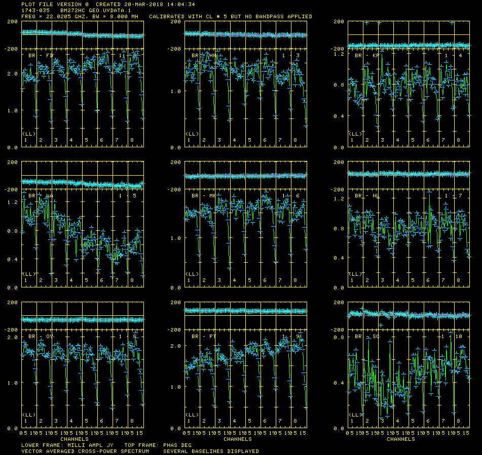
Cross power spectrum plot of 1743-035 showing phase corrections.
Find and remove instrumental delay by running VLBAMPCL, that runs FRING and CLCAL.
- default vlbampcl
- getn 2
- calsour '1743-035' '
- timer 0 7 15 8 0 7 16 01 ➜ scan with good fringes we found in POSSM plots.
- refant 2 ➜ choose reference antenna from in the middle of array, FD (antenna 2) is a good choice.
- gainu 0 ➜ apply highest CL table.
- inp
- vlbampcl
At this point you should check on the calibration:
- First check you have no failed solutions. At the end of the FRING run it should tell you how many "good" and "failed" solutions it has found. For this step there must be no failed solutions, failed solutions in this step mean that whatever antenna the failed solution was on is deleted from your data. For this data there should be "80 good solutions".
FRING1: Time=   0/ 07 15 35, Polarization = 1
FRING1: Found       80 good solutions
FRING1: Adjusting solutions to a common reference antenna
FRING1: Appears to have ended successfully
- check solutions in POSSM, the jumps in phase between the IFs should be gone. The phases may also be flattened.
- tget possm ➜ to "get" all the inputs from the last run (it was run when we ran the procedure VLBACRPL).
- gainu 5
- baseline 0
- sources '1743-035' '
- inp
- go
Again hit "B" a few times. As you can see from Figure 12, the phase jumps between the IF's are gone. Some sources will show a general phase slope across all the IF's. This is the multi-band delay that we will measure and fit for the zenith delay.
Determine Multi-Band Delay
Determine multi-band delay (MBD) by running FRING. This will take a few minutes.
- default fring
- getn 2
- refant 2
- docal 1; gainu 5
- aparm(5)=2 ➜ solve for the MBD.
- inp
- go
FRING will take some time to run and there will be a lot of failed solutions (~20%) here, but that is O.K.. :
FRING1: Found     3448 good solutions
FRING1: Failed on      736 solutions
FRING1: Adjusting solutions to a common reference antenna
FRING1: Appears to have ended successfully
Plot the Multi-Band Delay
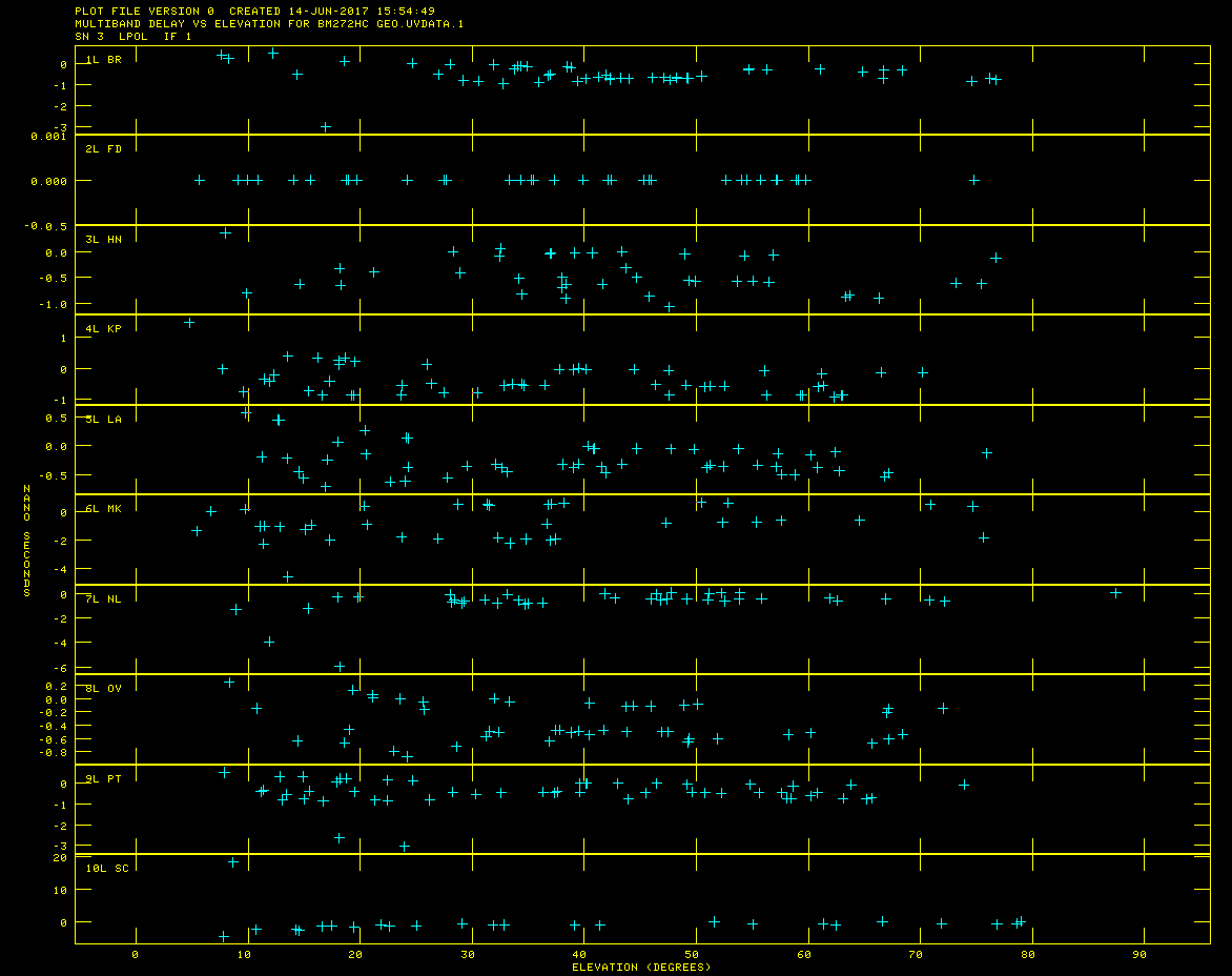
Multi-Band delay plot showing offset points that will need to be flagged.
Check MBD with SNPLT.
- default snplt
- getn 2
- inext 'sn'; invers 3
- nplots 10
- dotv 1
- opty 'mdel'➜ plot MBD.
- xaxis 2➜ plot verses elevation.
- inp
- tvin; go ➜ clear TV and run task
It is important that the MBD be correct because the fitting in DELZN can easily go wonky.
Figure 13 shows the resulting plot generated by SNPLT. Note that most MBD are between a fraction and a few ns. Large ones are probably wrong and should be clipped. There also should be a general trend from low to high elevations, although this is not always clear in the plot. The most obvious classic case is for SC as seen in Figure 13. Make note of the obviously bad points. Here, in Figure 13, there is one at BR (antenna 1, -3 ns), one at NL (antenna 7, -6 ns), two at PT (antenna 9, -3 ns), and one at SC (antenna 10, about 19 ns). Your solutions may vary, but you should get something qualitatively similar.
Flag Offset Data Points
Edit the MBD with SNEDT. SNEDT will only plot versus time, which is why we noted the bad points above.
- default snedt
- getn 2
- inext 'sn'; invers 3
- antuse 1 2 3 4 5 6 7 8 9 10
- dodelay 2
- inp
- go
Flag the points noted above. After having removed the bad points and exiting, a new solutions table (SN #4) should have been created (check with imh).
Inspect the Corrected Multi-Band Delays, run DELZN
Check MBD again with SNPLT.
- tget snplt
- invers 4
- tvin
- inp
- go
Looks OK, maybe some more flagging needed (SC with a data point at -4 ns), but lets see how DELZN does.
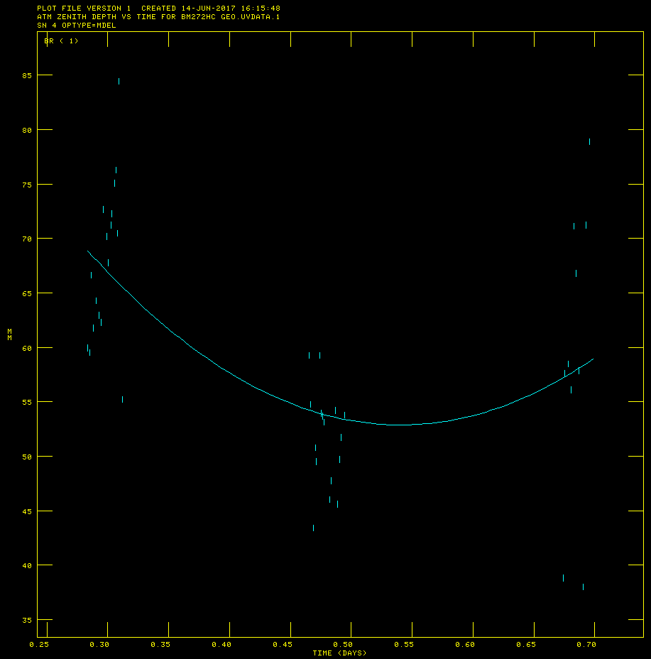
Polynomial fit plot (PL 1) for the Brewster VLBA antenna, which is generated by running DELZN.
- Solve for zenith and clock delays with DELZN.
- default delzn
- getn 2
- snver 4➜ SN table with edited MBD
- gainv 5➜ CL table to copy and correct.
- aparm 0 3 2 1 1 10➜ plot zenith atmos. delay; use 3 polynomial terms to fit atmosphere; use 2 polynomial terms to fit clock; create CL table; correct both atmosphere and clock; use 10 iterations of robust fitting.
- opty 'mdel'➜ fit MBD.
- outfi 'FITS:delzn.clor ➜ file to read in with CLCOR; note if you leave off the closing ' the outfi retains the case.
- dotv -1➜ don't plot to TV, only make PL files.
- inp
- go
The generated plot files can be viewed with TVPL.
- Plot generated PL files with TVPL
- default tvpl
- getn 2
- for plver= 1 to 9; go tvpl; tvps; end
The plots should get displayed on the AIPSTV display (Figure 14). Hit "D" to scroll through the plots.
DELZN makes plots that I don't find particularly useful to evaluate the quality of the fit. The best way to evaluate this (other than applying it to the astrometric data and see if it improves things) is to apply the CL table that DELZN produces to the GEO data and see if it flattens the MBD across all the IF's.
- Plot GEO data with CL table 5, and compare it to CL table 6 which was generated by DELZN
- tget possm
- getn 2
- gainuse 5
- source '1751+093' '
- timer 0 11 10 42 0 11 12 15
- inp
- go
where the source and time range have been chosen to illustrate the differences clearly. After scrolling through the plots by pressing "B", or exiting with "D", generate plots with CL 6.
- gainuse 6
- go
Compare the phases to the same source when applying CL 6. As you can see in Figure 15b, the results look quite good after applying CL 6.
Solution transfer: Apply Delay Corrections
Now we transfer these solutions to the target dataset.
This is where it gets a little complicated (although not much). Now we must apply the solutions we derived above on the GEO data, to the original data with the target in it. The target data should have all the calibration done except the final fringe fit (CL table version 1). Then we can compare two versions/methods of this data reduction: images of the target data with previously final fringe fit done (CL table ver 2; non-DELZNed data), with the images of the target data to which we transferred the GEO solution (DELZNed data), and see which one is better.
Use "imh" on the multi-source TARGET (SPLATed) data to see how many CL tables there are (two - if you followed this guide to the letter). We want to apply the DELZN solution to the CL table immediately before the final fringe fit we performed to that data.
Apply the zenith delay correction with CLCOR.
- default clcor
- getn 4
- opco 'atmo' ➜ read in a file of atmospheric and clock delay corrections and apply them to the given CL table.
- gainv 1; gainu 0 ➜ input CL#1; generate a new CL table (CL 3).
- infile 'FITS:delzn.clor ➜ file with corrections we created earlier with the GEO data.
- inp
- go
CLCOR will say it has created CL table #3. Use this for further calibration, i.e. skip CL#2.
Fringe Fit Data
Now, do the global fringe fit with FRING on the DELZNed target data. This is where vput/vget come in handy, if you didn't do the vput, then repeat step previous FRING done on BM272HC.SPLAT.1 (Section 6.17), but change the gainuse parameter as shown below.
- vnum 1; vget fring
- gainu 3
- inp
- go
Again, check the number of good and failed solutions:
 FRING1: Found     4498 good solutions
 FRING1: Failed on       42 solutions
 FRING1: Adjusting solutions to a common reference antenna
You should get something similar but not necessarily exactly the same numbers of good and failed solutions. A small percentage of failed solutions are fine at this point.
Apply Calibrations
Apply calibration to tables with CLCAL. Again, either use vnum/vget, or repeat CLCAL step from above (from Section 6.18), changing parameters as shown below.
- vnum 1; vget clcal
- snver 2
- gainv 3
- gainu 4
- inp
- go
Split the Data
Apply calibration to data with SPLIT. Here we can use tget because SPLIT has not been used since the last time we ran it on this data. Again repeat step 6.19 if you can't do this.
- tget split
- gainu 4 ➜ apply CL#4 to the data
- outcl 'delzn'
- inp
- go
Image J2007+4029
Image J2007+4029 with IMAGR.
- tget imagr
- getn 17
- cell 3e-5
- imsi 512
- dotv 1
- niter 1000
- im2parm 10 6 9 0.5
- bchan 0; echan 0
- nchav 256
- inp
- go
Use the correct catalog number for J2007+4029 DELZN version. It was 17 on my disk. Then run IMAGR and compare the new image to the one made without the correction (Figure 16a).
As you can see, the image after the correction (Figure 16b) has a lower noise level and a source with a higher peak. Bad phases spread the flux around the image and make the noise level higher and source flux lower as well as shifting the position of the source.

