VLA Data Combination-W49A-CASA6.2.0: Difference between revisions
| (16 intermediate revisions by 2 users not shown) | |||
| Line 5: | Line 5: | ||
A perfect image requires measurement of all spatial scales, which is equivalent to filling in the complete uv plane. Unfortunately, this can never be achieved with an aperture synthesis interferometer, although a large number of baselines, long integration times, and multi-frequency-synthesis are all good approaches to increase the uv-coverage. One method to obtain more baselines is to observe in different array configurations and to combine the data afterwards. Deconvolution algorithms are then given good starting conditions to interpolate across the gaps in the uv-plane to achieve an image that combines the surface brightness sensitivity of the compact baselines with the spatial resolution of the extended baselines. | A perfect image requires measurement of all spatial scales, which is equivalent to filling in the complete uv plane. Unfortunately, this can never be achieved with an aperture synthesis interferometer, although a large number of baselines, long integration times, and multi-frequency-synthesis are all good approaches to increase the uv-coverage. One method to obtain more baselines is to observe in different array configurations and to combine the data afterwards. Deconvolution algorithms are then given good starting conditions to interpolate across the gaps in the uv-plane to achieve an image that combines the surface brightness sensitivity of the compact baselines with the spatial resolution of the extended baselines. | ||
The VLA can be configured into [https://go.nrao.edu/vla-res four principal array configurations] | The VLA can be configured into [https://go.nrao.edu/vla-res four principal array configurations]: A, B, C, and D. The A configuration is the most extended, and D is the most compact configuration. Consequently, A-configuration data exhibit the highest spatial resolution whereas D-configuration delivers the best surface brightness sensitivity and also images the largest scales of the sky brightness distribution. | ||
In this tutorial, we will combine data from all four VLA configurations (A, B, C, and D) that were observed in X-band continuum toward W49A, a massive star forming region in the Milky Way. | In this tutorial, we will combine data from all four VLA configurations (A, B, C, and D) that were observed in X-band continuum toward W49A, a massive star forming region in the Milky Way. | ||
| Line 133: | Line 133: | ||
Task listobs complete. Start time: 2021-09-10 10:01:51.648534 End time: 2021-09-10 10:01:51.932094 | Task listobs complete. Start time: 2021-09-10 10:01:51.648534 End time: 2021-09-10 10:01:51.932094 | ||
##### End Task: listobs ##### | ##### End Task: listobs ##### | ||
########################################## | |||
</pre> | </pre> | ||
| Line 138: | Line 140: | ||
The data were prepared for this tutorial to contain only one source, W49A, calibrated through the VLA pipeline (although, for the sake of this tutorial, no [https://casadocs.readthedocs.io/en/v6.2.0/api/tt/casatasks.manipulation.statwt.html statwt] task has been run, see below). To reduce the size of the files, the MS only contains one spectral window, binned into 64 2MHz channels around 8.4GHz (X-band). We also extracted the calibrated data, discarding the raw data and any model, such that the MS now only contains visibilities in the DATA column. The on-source integration time amounts to about 2.5h. Inspection of the other array configuration files show almost identical setups. Although the integration times between the different array configurations do not follow the 1:3:9:27 ratios that we discussed in the previous section, we can still combine the data without any problem. In the end, having a higher signal to noise ratio on the shorter baselines can only improve the overall combined image. | The data were prepared for this tutorial to contain only one source, W49A, calibrated through the VLA pipeline (although, for the sake of this tutorial, no [https://casadocs.readthedocs.io/en/v6.2.0/api/tt/casatasks.manipulation.statwt.html statwt] task has been run, see below). To reduce the size of the files, the MS only contains one spectral window, binned into 64 2MHz channels around 8.4GHz (X-band). We also extracted the calibrated data, discarding the raw data and any model, such that the MS now only contains visibilities in the DATA column. The on-source integration time amounts to about 2.5h. Inspection of the other array configuration files show almost identical setups. Although the integration times between the different array configurations do not follow the 1:3:9:27 ratios that we discussed in the previous section, we can still combine the data without any problem. In the end, having a higher signal to noise ratio on the shorter baselines can only improve the overall combined image. | ||
To better understand the data, let's check the uv-coverage of each of the | To better understand the data, let's check the uv-coverage of each of the four datasets. For faster plotting, we only plot channel 32 near the center of each spectral window. All plots are on the same scale: | ||
<source lang="python"> | <source lang="python"> | ||
| Line 144: | Line 146: | ||
# A-config: | # A-config: | ||
plotms(vis='A-W49A.ms',xaxis='Uwave',yaxis='Vwave',spw='0:32',plotrange=[-1000000,1000000,-1000000,1000000]) | plotms(vis='A-W49A.ms',xaxis='Uwave',yaxis='Vwave',spw='0:32',plotrange=[-1000000,1000000,-1000000,1000000]) | ||
# B-config | # B-config | ||
plotms(vis='B-W49A.ms',xaxis='Uwave',yaxis='Vwave',spw='0:32',plotrange=[-1000000,1000000,-1000000,1000000]) | plotms(vis='B-W49A.ms',xaxis='Uwave',yaxis='Vwave',spw='0:32',plotrange=[-1000000,1000000,-1000000,1000000]) | ||
# C-config: | # C-config: | ||
plotms(vis='C-W49A.ms',xaxis='Uwave',yaxis='Vwave',spw='0:32',plotrange=[-1000000,1000000,-1000000,1000000]) | plotms(vis='C-W49A.ms',xaxis='Uwave',yaxis='Vwave',spw='0:32',plotrange=[-1000000,1000000,-1000000,1000000]) | ||
# D-config: | # D-config: | ||
plotms(vis='D-W49A.ms',xaxis='Uwave',yaxis='Vwave',spw='0:32',plotrange=[-1000000,1000000,-1000000,1000000]) | plotms(vis='D-W49A.ms',xaxis='Uwave',yaxis='Vwave',spw='0:32',plotrange=[-1000000,1000000,-1000000,1000000]) | ||
</source> | </source> | ||
The uv-coverage plots are shown in Fig. 1a-d using a common scale. The longest baseline in each array differs by about a factor of 3, as expected, between the VLA A, B, | The uv-coverage plots are shown in Fig. 1a-d using a common scale. The longest baseline in each array differs by about a factor of 3, as expected, between the VLA A, B, C, and D configurations. | ||
| Line 182: | Line 174: | ||
# In CASA | # In CASA | ||
# A-config: | # A-config: | ||
tclean(vis='A-W49A.ms',imagename='Aonly',cell='0.05arcsec',imsize=[1280,1280],weighting='briggs', | |||
robust=0,specmode='mfs',phasecenter='J2000 19:10:14 +09.06.13.7') | |||
# B-config: | |||
tclean(vis='B-W49A.ms',imagename='Bonly',cell='0.05arcsec',imsize=[1280,1280],weighting='briggs',robust=0,specmode='mfs',phasecenter='J2000 19:10:14 +09.06.13.7') | tclean(vis='B-W49A.ms',imagename='Bonly',cell='0.05arcsec',imsize=[1280,1280],weighting='briggs', | ||
tclean(vis='C-W49A.ms',imagename='Conly',cell='0.05arcsec',imsize=[1280,1280],weighting='briggs',robust=0,specmode='mfs',phasecenter='J2000 19:10:14 +09.06.13.7') | robust=0,specmode='mfs',phasecenter='J2000 19:10:14 +09.06.13.7') | ||
tclean(vis='D-W49A.ms',imagename='Donly',cell='0.05arcsec',imsize=[1280,1280],weighting='briggs',robust=0,specmode='mfs',phasecenter='J2000 19:10:14 +09.06.13.7') | |||
# C-config: | |||
tclean(vis='C-W49A.ms',imagename='Conly',cell='0.05arcsec',imsize=[1280,1280],weighting='briggs', | |||
robust=0,specmode='mfs',phasecenter='J2000 19:10:14 +09.06.13.7') | |||
# D-config: | |||
tclean(vis='D-W49A.ms',imagename='Donly',cell='0.05arcsec',imsize=[1280,1280],weighting='briggs', | |||
robust=0,specmode='mfs',phasecenter='J2000 19:10:14 +09.06.13.7') | |||
</source> | </source> | ||
| Line 205: | Line 206: | ||
== Check and Adjust the Visibility Weights == | == Check and Adjust the Visibility Weights == | ||
VLA weights are currently based only on channel width and correlator integration time. In the future, the VLA may use the switched power measurements to derive absolute calibrated weights. At the moment, however, the VLA weights need to be taken as being relative to each other. The relative sensitivity within an observation is measured by the gain, so weights of single, continuous observations are self-consistent. It is important to adjust the weights between ''separate'' observations as they will be on different scales. | VLA visibility weights are currently based only on channel width and correlator integration time. In the future, the VLA may use the switched power measurements to derive absolute calibrated weights. At the moment, however, the VLA weights need to be taken as being relative to each other. The relative sensitivity within an observation is measured by the gain, so weights of single, continuous observations are self-consistent. It is important to adjust the weights between ''separate'' observations as they will potentially be on different scales. | ||
Let's have a look at the weights of the different datasets. We will plot the weights as a function of uv-distance in a single central channel for improved plotting time: | Let's have a look at the weights of the different datasets. We will plot the weights as a function of uv-distance in a single central channel for improved plotting time: | ||
| Line 233: | Line 234: | ||
</source> | </source> | ||
Fig. 3a-d shows | Fig. 3a-d shows the weights and they are as described above. | ||
{| | {| | ||
| Line 253: | Line 254: | ||
3) Calculate the weights based on the rms of the cross-polarization products (currently not supported in [https://casadocs.readthedocs.io/en/v6.2.0/api/tt/casatasks.manipulation.statwt.html statwt]). | 3) Calculate the weights based on the rms of the cross-polarization products (currently not supported in [https://casadocs.readthedocs.io/en/v6.2.0/api/tt/casatasks.manipulation.statwt.html statwt]). | ||
We recommend to reset the weights when there are strong sources present in the data as they will change the rms of the visibilities and the rms will not be representative of the noise anymore. Without strong sources, [https://casadocs.readthedocs.io/en/v6.2.0/api/tt/casatasks.manipulation.statwt.html statwt] should deliver better results. The third option may work both cases, but requires full polarization observations and calibrations. For this guide we will | We recommend to reset the weights when there are strong sources present in the data as they will change the rms of the visibilities and the rms will not be representative of the noise anymore. Without strong sources, [https://casadocs.readthedocs.io/en/v6.2.0/api/tt/casatasks.manipulation.statwt.html statwt] should deliver better results. The third option may work for both cases, but requires full polarization observations and calibrations. For this guide we will follow the [https://casadocs.readthedocs.io/en/v6.2.0/api/tt/casatasks.manipulation.statwt.html statwt] path as an example. But the user should be aware of the different options for optimized imaging. | ||
| Line 259: | Line 260: | ||
[https://casadocs.readthedocs.io/en/v6.2.0/api/tt/casatasks.manipulation.statwt.html statwt] will bring all the weights of all observations on the same scale. The task recalculates the visibility weights based on the inverse of their rms. Task [https://casadocs.readthedocs.io/en/v6.2.0/api/tt/casatasks.manipulation.statwt.html statwt] is part of the [https://go.nrao.edu/vla-pipe VLA pipeline], so the pipelined data may already have recalculated weights and this | [https://casadocs.readthedocs.io/en/v6.2.0/api/tt/casatasks.manipulation.statwt.html statwt] will bring all the weights of all observations on the same scale. The task recalculates the visibility weights based on the inverse of their rms. Task [https://casadocs.readthedocs.io/en/v6.2.0/api/tt/casatasks.manipulation.statwt.html statwt] is part of the [https://go.nrao.edu/vla-pipe VLA pipeline], so the pipelined data may already have recalculated weights and this step can be skipped. It does not hurt though, to re-run [https://casadocs.readthedocs.io/en/v6.2.0/api/tt/casatasks.manipulation.statwt.html statwt]. | ||
For more information on weights, see [https://casadocs.readthedocs.io/en/stable/notebooks/data_weights.html definition of data weights] | For more information on weights, see [https://casadocs.readthedocs.io/en/stable/notebooks/data_weights.html definition of data weights]. | ||
Task [https://casadocs.readthedocs.io/en/v6.2.0/api/tt/casatasks.manipulation.statwt.html statwt] will be executed on each MS. The default setting calculates the weight based on the rms of each scan and spectral window. This setting works quite well for continuum observations. We would like to note though that for spectral line data the ''fitspw'' parameter should be set to exclude the line from the calculations. Otherwise, strong lines will be down-weighted. | Task [https://casadocs.readthedocs.io/en/v6.2.0/api/tt/casatasks.manipulation.statwt.html statwt] will be executed on each MS. The default setting calculates the weight based on the rms of each scan and spectral window. This setting works quite well for continuum observations. We would like to note though that for spectral line data the ''fitspw'' parameter should be set to exclude the line from the calculations. Otherwise, strong lines will be down-weighted. | ||
| Line 270: | Line 271: | ||
# A-config: | # A-config: | ||
statwt(vis='A-W49A.ms',datacolumn='data') | statwt(vis='A-W49A.ms',datacolumn='data') | ||
# B-config | # B-config | ||
statwt(vis='B-W49A.ms',datacolumn='data') | statwt(vis='B-W49A.ms',datacolumn='data') | ||
# C-config: | # C-config: | ||
statwt(vis='C-W49A.ms',datacolumn='data') | statwt(vis='C-W49A.ms',datacolumn='data') | ||
# D-config: | # D-config: | ||
statwt(vis='D-W49A.ms',datacolumn='data') | statwt(vis='D-W49A.ms',datacolumn='data') | ||
| Line 296: | Line 288: | ||
# A-config: | # A-config: | ||
plotms(vis='A-W49A.ms',spw='0:32',xaxis='uvwave',yaxis='wt',coloraxis='antenna1') | plotms(vis='A-W49A.ms',spw='0:32',xaxis='uvwave',yaxis='wt',coloraxis='antenna1') | ||
# B-config | # B-config | ||
plotms(vis='B-W49A.ms',spw='0:32',xaxis='uvwave',yaxis='wt',coloraxis='antenna1') | plotms(vis='B-W49A.ms',spw='0:32',xaxis='uvwave',yaxis='wt',coloraxis='antenna1') | ||
# C-config: | # C-config: | ||
plotms(vis='C-W49A.ms',spw='0:32',xaxis='uvwave',yaxis='wt',coloraxis='antenna1') | plotms(vis='C-W49A.ms',spw='0:32',xaxis='uvwave',yaxis='wt',coloraxis='antenna1') | ||
# D-config: | |||
# | |||
plotms(vis='D-W49A.ms',spw='0:32',xaxis='uvwave',yaxis='wt',coloraxis='antenna1') | plotms(vis='D-W49A.ms',spw='0:32',xaxis='uvwave',yaxis='wt',coloraxis='antenna1') | ||
</source> | </source> | ||
| Line 328: | Line 311: | ||
== Combining and Imaging All Data == | == Combining and Imaging All Data == | ||
We will now create a combined image of all | We will now create a combined image of all four re-weighted datasets. | ||
First, let's check the new uv-coverage. We concatenate the data with [https://casadocs.readthedocs.io/en/v6.2.0/api/tt/casatasks.manipulation.concat.html concat] | First, let's check the new uv-coverage. We concatenate the data with [https://casadocs.readthedocs.io/en/v6.2.0/api/tt/casatasks.manipulation.concat.html concat]: | ||
<source lang="python"> | <source lang="python"> | ||
# In CASA | # In CASA | ||
concat(vis=['A-W49A.ms','B-W49A.ms','C-W49A.ms','D-W49A'],concatvis='ABCD-W49A.ms') | concat(vis=['A-W49A.ms','B-W49A.ms','C-W49A.ms','D-W49A.ms'],concatvis='ABCD-W49A.ms') | ||
</source> | </source> | ||
| Line 344: | Line 327: | ||
</source> | </source> | ||
Fig. 5 shows the combined uv-coverage, which extends to A-configuration baselines but with a much higher density at the intermediate and | Fig. 5 shows the combined uv-coverage, which extends to A-configuration baselines but with a much higher density at the intermediate and short baselines contributed from B, C, and D configurations. | ||
{| | {| | ||
| Line 351: | Line 334: | ||
Although [https://casadocs.readthedocs.io/en/v6.2.0/api/tt/casatasks.manipulation.concat.html concat] merges all | Although [https://casadocs.readthedocs.io/en/v6.2.0/api/tt/casatasks.manipulation.concat.html concat] merges all four MSs into a single one, it is actually not a required step before imaging. Task [https://casadocs.readthedocs.io/en/v6.2.0/api/tt/casatasks.imaging.tclean.html tclean] will take care of the combination when all datasets are specified as a list. Tclean will also perform the spectral regridding of all datasets on the fly, in particular in ''mode="velocity"'' or ''mode="frequency"''. There's no need to run [https://casadocs.readthedocs.io/en/v6.2.0/api/tt/casatasks.manipulation.cvel.html cvel]/[https://casadocs.readthedocs.io/en/v6.2.0/api/tt/casatasks.manipulation.cvel2.html cvel2] (or [https://casadocs.readthedocs.io/en/v6.2.0/api/tt/casatasks.manipulation.mstransform.html mstransform]) to Doppler correct the MSs beforehand. | ||
We will now create a combined image in [https://casadocs.readthedocs.io/en/v6.2.0/api/tt/casatasks.imaging.tclean.html tclean]. The ''threshold'' parameter was derived by a previous run of [https://casadocs.readthedocs.io/en/v6.2.0/api/tt/casatasks.imaging.tclean.html tclean] on the combined MS for which we determined the rough rms noise. For our threshold, we will use the rms noise multiplied by a factor of ~2.5. | We will now create a combined image in [https://casadocs.readthedocs.io/en/v6.2.0/api/tt/casatasks.imaging.tclean.html tclean]. The ''threshold'' parameter was derived by a previous run of [https://casadocs.readthedocs.io/en/v6.2.0/api/tt/casatasks.imaging.tclean.html tclean] on the combined MS for which we determined the rough rms noise. For our threshold, we will use the rms noise multiplied by a factor of ~2.5. | ||
| Line 374: | Line 357: | ||
== Tips for Selfcal == | == Tips for Selfcal == | ||
If the source has a bright nucleus or, more generally, a bright unresolved emission, start with the A array data, selfcal, then add B array, selfcal again, and so on. This procedure starts with a high model flux that is increased further. If the source is mostly diffuse, then there is not much signal in the A array data, so start with the D array, selfcal, then add C array, selfcal, and so on. Each selfcal step should be phase only first with maybe two or more iterations. At the end of each selfcal step, a phase+amplitude selfcal can be attempted, before merging in the next array configuration data. After each merge the selfcal steps can be repeated. | If the source has a bright nucleus or, more generally, a bright unresolved emission, start with the A array data, selfcal, then add B array, selfcal again, and so on. This procedure starts with a high model flux that is increased further. If the source is mostly diffuse, then there is not much signal in the A array data, so start with the D array, selfcal, then add C array, selfcal, and so on. Each selfcal step should be phase-only first with maybe two or more iterations. At the end of each selfcal step, a phase+amplitude selfcal can be attempted, before merging in the next array configuration data. After each merge the selfcal steps can be repeated. General selfcal procedures are outlined in the [https://casaguides.nrao.edu/index.php?title=Karl_G._Jansky_VLA_Tutorials#Self-calibration_of_VLA_Data Self-Calibration topical guide]. | ||
Latest revision as of 23:56, 5 October 2021
This tutorial was created and tested using CASA 6.2.0
Introduction
A perfect image requires measurement of all spatial scales, which is equivalent to filling in the complete uv plane. Unfortunately, this can never be achieved with an aperture synthesis interferometer, although a large number of baselines, long integration times, and multi-frequency-synthesis are all good approaches to increase the uv-coverage. One method to obtain more baselines is to observe in different array configurations and to combine the data afterwards. Deconvolution algorithms are then given good starting conditions to interpolate across the gaps in the uv-plane to achieve an image that combines the surface brightness sensitivity of the compact baselines with the spatial resolution of the extended baselines.
The VLA can be configured into four principal array configurations: A, B, C, and D. The A configuration is the most extended, and D is the most compact configuration. Consequently, A-configuration data exhibit the highest spatial resolution whereas D-configuration delivers the best surface brightness sensitivity and also images the largest scales of the sky brightness distribution.
In this tutorial, we will combine data from all four VLA configurations (A, B, C, and D) that were observed in X-band continuum toward W49A, a massive star forming region in the Milky Way.
Typical Observing Times
When an object is being observed by the VLA in different array configurations, on-source integration times are ideally matched to reach a common surface brightness sensitivity for all scales. Adjacent VLA configurations result in synthesized beams that differ in linear size by approximately a factor of 3. The beam areas therefore change by factors of ~10 and the more extended configuration would ideally need to have 10 times more integration time than the next compact one. This, however, is frequently not very practical and it turns out that integration times that differ by factors of ~3 deliver data that can be satisfactorily combined. This combination matches the sensitivity of overlapping VLA visibilities when the data are convolved to the same scales.
Although overlapping uv-coverages are essential for the best imaging, it is possible to combine non-overlapping data if one understands that some spacings are not present and that the adjustment of the individual datasets is somewhat subjective. Weighting will be primarily achieved during imaging by the Briggs scheme that allows one to adjust imaging weights between the natural (weighting by the number of visibilities that are gridded in each cell) and uniform (weighting by the cells themselves) extremes.
Additionally, each visibility exhibits weights that should only depend on correlator integration time, bandwidth, and system temperature (Tsys). Note that the VLA does not apply Tsys in the online system. Visibility weights between different observations will therefore need to be adjusted, as described below, before they can be combined.
The Data
We will be combining four different datasets, X-band A, B, C, and D configuration data. The data were all calibrated and the science target split out.
The calibrated measurement sets can be downloaded here:
https://casa.nrao.edu/Data/EVLA/combination/VLA-combination-W49A.tar.gz (3.0G)
As a first step download the file above, then untar:
# In a Terminal
tar -xzvf VLA-combination-W49A.tar.gz
This will unpack four MeasurementSets (MSs), one for each array configuration:
A-W49A.ms
B-W49A.ms
C-W49A.ms
D-W49A.ms
Initial Imaging
We will inspect the data and create separate images to better understand the image parameters such as on-source integration time, resolution, and rms.
Start CASA:
# In a Terminal
casa
As a first step, let's have a look at the 'listobs' output for the different MSs. For example, the A-configuration MS has the following structure:
# In CASA
listobs(vis='A-W49A.ms')
  ##########################################
  ##### Begin Task: listobs            #####
  listobs( vis='A-W49A.ms', selectdata=True, spw='', field='', antenna='', uvrange='', timerange='', correlation='', scan='', intent='', feed='', array='', observation='', verbose=True, listfile='', listunfl=False, cachesize=50.0, overwrite=False )
  ================================================================================
             MeasurementSet Name:  /lustre/aoc/sciops/jott/casa/combination-2021/data/vis-small3/A-W49A.ms      MS Version 2
  ================================================================================
     Observer: Dr. Chris De Pree     Project: uid://evla/pdb/30105074
  Observation: EVLA
  Computing scan and subscan properties...
  Data records: 764478       Total elapsed time = 8973 seconds
     Observed from   24-Jun-2015/07:32:30.0   to   24-Jun-2015/10:02:03.0 (UTC)

     ObservationID = 0         ArrayID = 0
    Date        Timerange (UTC)          Scan  FldId FieldName             nRows     SpwIds   Average Interval(s)    ScanIntent
    24-Jun-2015/07:32:30.0 - 07:42:24.0     4      0 W49A                     69498  [0]  [3] [OBSERVE_TARGET#UNSPECIFIED]
                07:42:27.0 - 07:47:24.0     5      0 W49A                     34749  [0]  [3] [OBSERVE_TARGET#UNSPECIFIED]
                07:49:27.0 - 07:59:21.0     7      0 W49A                     69498  [0]  [3] [OBSERVE_TARGET#UNSPECIFIED]
                07:59:24.0 - 08:04:21.0     8      0 W49A                     34749  [0]  [3] [OBSERVE_TARGET#UNSPECIFIED]
                08:06:24.0 - 08:16:18.0    10      0 W49A                     69498  [0]  [3] [OBSERVE_TARGET#UNSPECIFIED]
                08:16:21.0 - 08:21:18.0    11      0 W49A                     34749  [0]  [3] [OBSERVE_TARGET#UNSPECIFIED]
                08:23:21.0 - 08:33:18.0    13      0 W49A                     69849  [0]  [3] [OBSERVE_TARGET#UNSPECIFIED]
                08:33:21.0 - 08:38:15.0    14      0 W49A                     34398  [0]  [3] [OBSERVE_TARGET#UNSPECIFIED]
                08:40:18.0 - 08:50:15.0    16      0 W49A                     69849  [0]  [3] [OBSERVE_TARGET#UNSPECIFIED]
                08:50:18.0 - 08:55:12.0    17      0 W49A                     34398  [0]  [3] [OBSERVE_TARGET#UNSPECIFIED]
                08:57:15.0 - 09:07:12.0    19      0 W49A                     69849  [0]  [3] [OBSERVE_TARGET#UNSPECIFIED]
                09:07:15.0 - 09:12:09.0    20      0 W49A                     34398  [0]  [3] [OBSERVE_TARGET#UNSPECIFIED]
                09:40:09.0 - 09:50:03.0    25      0 W49A                     69498  [0]  [3] [OBSERVE_TARGET#UNSPECIFIED]
                09:50:06.0 - 09:55:03.0    26      0 W49A                     34749  [0]  [3] [OBSERVE_TARGET#UNSPECIFIED]
                09:57:06.0 - 10:02:03.0    28      0 W49A                     34749  [0]  [3] [OBSERVE_TARGET#UNSPECIFIED]
             (nRows = Total number of rows per scan)
  Fields: 1
    ID   Code Name                RA               Decl           Epoch   SrcId      nRows
    0    NONE W49A                19:10:12.930999 +09.06.11.88200 J2000   0         764478
  Spectral Windows:  (1 unique spectral windows and 1 unique polarization setups)
    SpwID  Name           #Chans   Frame   Ch0(MHz)  ChanWid(kHz)  TotBW(kHz) CtrFreq(MHz) BBC Num  Corrs
    0      EVLA_X#B0D0#11     64   TOPO    8372.479      2000.000    128000.0   8435.4793       15  RR  LL
  Sources: 1
    ID   Name                SpwId RestFreq(MHz)  SysVel(km/s)
    0    W49A                0     9816.865       8
  Antennas: 27:
    ID   Name  Station   Diam.    Long.         Lat.                Offset from array center (m)                ITRF Geocentric coordinates (m)
                                                                       East         North     Elevation               x               y               z
    0    ea01  N64       25.0 m   -107.37.58.7  +34.02.20.5      -1382.3871    15410.1384      -40.6410 -1599855.687000 -5033332.368600  3567636.613800
    1    ea02  N16       25.0 m   -107.37.10.9  +33.54.48.0       -155.8524     1426.6393       -9.3842 -1601061.957600 -5041175.881400  3556058.033100
    2    ea03  W48       25.0 m   -107.42.44.3  +33.50.52.1      -8707.9476    -5861.7878       15.5283 -1610451.932800 -5042471.123800  3550021.055800
    3    ea04  E40       25.0 m   -107.32.35.4  +33.52.16.9       6908.8199    -3240.7429       39.0197 -1595124.937100 -5045829.476200  3552210.683600
    4    ea05  E72       25.0 m   -107.24.42.3  +33.49.18.0      19041.8648    -8769.1806        4.7639 -1584460.883200 -5052385.614800  3547600.041100
    5    ea06  N40       25.0 m   -107.37.29.5  +33.57.44.4       -633.6056     6878.6057      -20.7877 -1600592.749000 -5038121.341300  3560574.846200
    6    ea07  N72       25.0 m   -107.38.10.5  +34.04.12.2      -1685.6797    18861.8360      -43.4978 -1599557.928700 -5031396.353400  3570494.743400
    7    ea08  E64       25.0 m   -107.27.00.1  +33.50.06.7      15507.6019    -7263.7123       67.2037 -1587600.192200 -5050575.870700  3548885.413900
    8    ea09  W08       25.0 m   -107.37.21.6  +33.53.53.0       -432.1156     -272.1458       -1.4994 -1601614.091200 -5042001.656900  3554652.514300
    9    ea10  E32       25.0 m   -107.34.01.5  +33.52.50.3       4701.6612    -2209.7048       25.2200 -1597053.118400 -5044604.692200  3553059.011100
    10   ea11  W24       25.0 m   -107.38.49.0  +33.53.04.0      -2673.3543    -1784.5861       10.4723 -1604008.747100 -5042135.805100  3553403.716300
    11   ea12  N32       25.0 m   -107.37.22.0  +33.56.33.6       -441.7251     4689.9820      -16.9255 -1600781.044100 -5039347.437000  3558761.543300
    12   ea13  W16       25.0 m   -107.37.57.4  +33.53.33.0      -1348.7131     -890.6107        1.2990 -1602592.853500 -5042054.989100  3554140.713000
    13   ea14  E08       25.0 m   -107.36.48.9  +33.53.55.1        407.8280     -206.0296       -3.2233 -1600801.931400 -5042219.381700  3554706.431200
    14   ea15  E24       25.0 m   -107.35.13.4  +33.53.18.1       2858.1759    -1349.1337       13.7125 -1598663.094300 -5043581.381100  3553767.012000
    15   ea16  W64       25.0 m   -107.46.20.1  +33.48.50.9     -14240.7524    -9606.2900       17.0885 -1616361.575500 -5042770.516600  3546911.419900
    16   ea17  N24       25.0 m   -107.37.16.1  +33.55.37.7       -290.3645     2961.8847      -12.2406 -1600930.072900 -5040316.384900  3557330.407200
    17   ea18  W72       25.0 m   -107.48.24.0  +33.47.41.2     -17419.4641   -11760.2694       14.9442 -1619757.299900 -5042937.656400  3545120.392300
    18   ea19  W40       25.0 m   -107.41.13.5  +33.51.43.1      -6377.9723    -4286.7839        8.2107 -1607962.451800 -5042338.204100  3551324.945500
    19   ea20  N48       25.0 m   -107.37.38.1  +33.59.06.2       -855.2671     9405.9613      -25.9164 -1600374.881000 -5036704.217500  3562667.893900
    20   ea21  E56       25.0 m   -107.29.04.1  +33.50.54.9      12327.6481    -5774.7445       42.6332 -1590380.599000 -5048810.261300  3550108.444300
    21   ea23  E16       25.0 m   -107.36.09.8  +33.53.40.0       1410.0345     -673.4704       -0.7961 -1599926.106100 -5042772.964400  3554319.787600
    22   ea24  W32       25.0 m   -107.39.54.8  +33.52.27.2      -4359.4410    -2923.1315       11.7693 -1605808.637100
    23   ea25  W56       25.0 m   -107.44.26.7  +33.49.54.6     -11333.1991    -7637.6832       15.3636 -1613255.391400 -5042613.097800  3548545.906000
    24   ea26  E48       25.0 m   -107.30.56.1  +33.51.38.4       9456.6036    -4431.6334       37.9266 -1592894.077600 -5047229.118200  3551221.221000
    25   ea27  N08       25.0 m   -107.37.07.5  +33.54.15.8        -68.9101      433.1984       -5.0732 -1601147.939700 -5041733.820400  3555235.956600
    26   ea28  N56       25.0 m   -107.37.47.9  +34.00.38.4      -1105.2275    12254.3062      -34.2445 -1600128.402500 -5035104.139200  3565024.670400
  Result listobs: True
  Task listobs complete. Start time: 2021-09-10 10:01:51.648534 End time: 2021-09-10 10:01:51.932094
  ##### End Task: listobs              #####
  ##########################################
The data were prepared for this tutorial to contain only one source, W49A, calibrated through the VLA pipeline (although, for the sake of this tutorial, no statwt task has been run, see below). To reduce the size of the files, the MS only contains one spectral window, binned into 64 2MHz channels around 8.4GHz (X-band). We also extracted the calibrated data, discarding the raw data and any model, such that the MS now only contains visibilities in the DATA column. The on-source integration time amounts to about 2.5h. Inspection of the other array configuration files show almost identical setups. Although the integration times between the different array configurations do not follow the 1:3:9:27 ratios that we discussed in the previous section, we can still combine the data without any problem. In the end, having a higher signal to noise ratio on the shorter baselines can only improve the overall combined image.
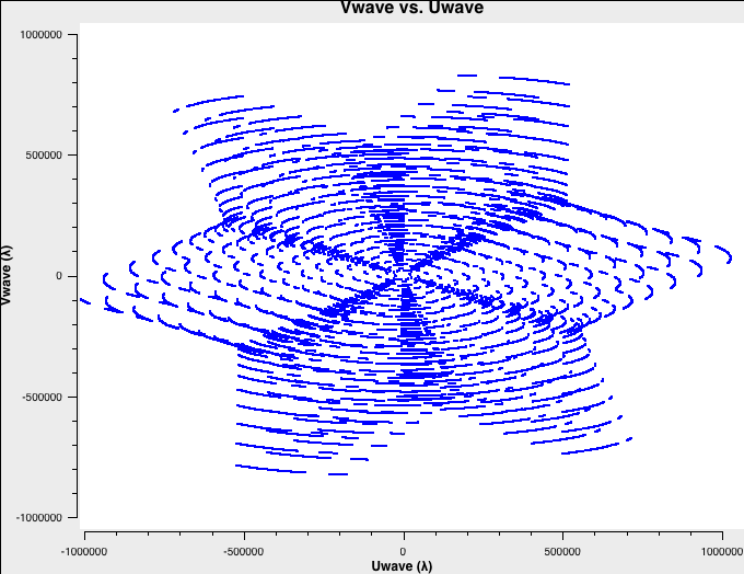
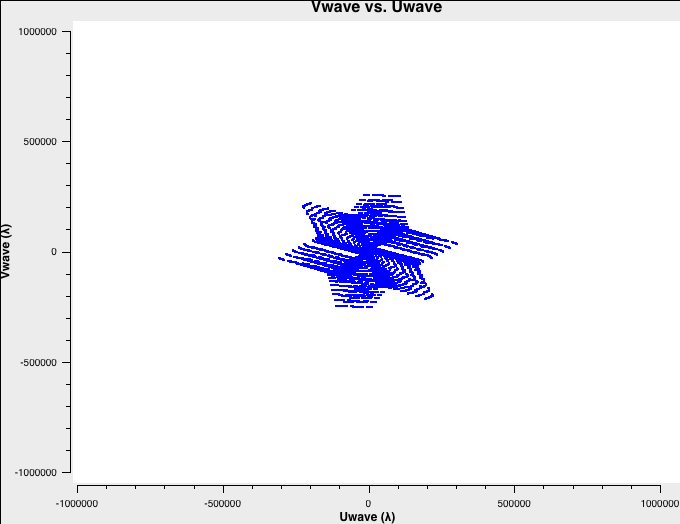
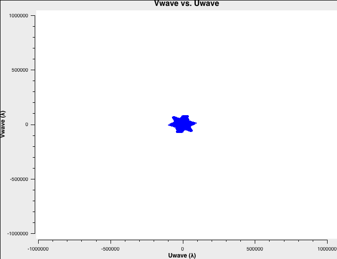
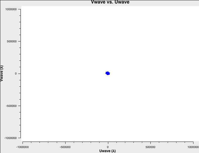
To better understand the data, let's check the uv-coverage of each of the four datasets. For faster plotting, we only plot channel 32 near the center of each spectral window. All plots are on the same scale:
# In CASA
# A-config:
plotms(vis='A-W49A.ms',xaxis='Uwave',yaxis='Vwave',spw='0:32',plotrange=[-1000000,1000000,-1000000,1000000])

# B-config
plotms(vis='B-W49A.ms',xaxis='Uwave',yaxis='Vwave',spw='0:32',plotrange=[-1000000,1000000,-1000000,1000000])

# C-config:
plotms(vis='C-W49A.ms',xaxis='Uwave',yaxis='Vwave',spw='0:32',plotrange=[-1000000,1000000,-1000000,1000000])

# D-config:
plotms(vis='D-W49A.ms',xaxis='Uwave',yaxis='Vwave',spw='0:32',plotrange=[-1000000,1000000,-1000000,1000000])
The uv-coverage plots are shown in Fig. 1a-d using a common scale. The longest baseline in each array differs by about a factor of 3, as expected, between the VLA A, B, C, and D configurations.
The next step is to determine the image quality, the synthesized beam, and the rms of each image. The images do not have to be perfectly deconvolved as we only would like to see how the combination will improve over the individual arrays.
To keep things simple, we will use common cell sizes of 0.05 arcsec, which samples well the A-configuration beam and oversamples the more compact configurations. We create images of 1280 pixels on each side, and we will tclean 1000 iterations (see the VLA CASA imaging guide for more sophisticated imaging parameter choices). We move the center of the image to the region with the main emission to avoid having to image a very large field of view:
# In CASA
# A-config:
tclean(vis='A-W49A.ms',imagename='Aonly',cell='0.05arcsec',imsize=[1280,1280],weighting='briggs',
       robust=0,specmode='mfs',phasecenter='J2000 19:10:14  +09.06.13.7')

# B-config:
tclean(vis='B-W49A.ms',imagename='Bonly',cell='0.05arcsec',imsize=[1280,1280],weighting='briggs',
       robust=0,specmode='mfs',phasecenter='J2000 19:10:14  +09.06.13.7')

# C-config:
tclean(vis='C-W49A.ms',imagename='Conly',cell='0.05arcsec',imsize=[1280,1280],weighting='briggs',
       robust=0,specmode='mfs',phasecenter='J2000 19:10:14  +09.06.13.7')

# D-config:
tclean(vis='D-W49A.ms',imagename='Donly',cell='0.05arcsec',imsize=[1280,1280],weighting='briggs',
       robust=0,specmode='mfs',phasecenter='J2000 19:10:14  +09.06.13.7')
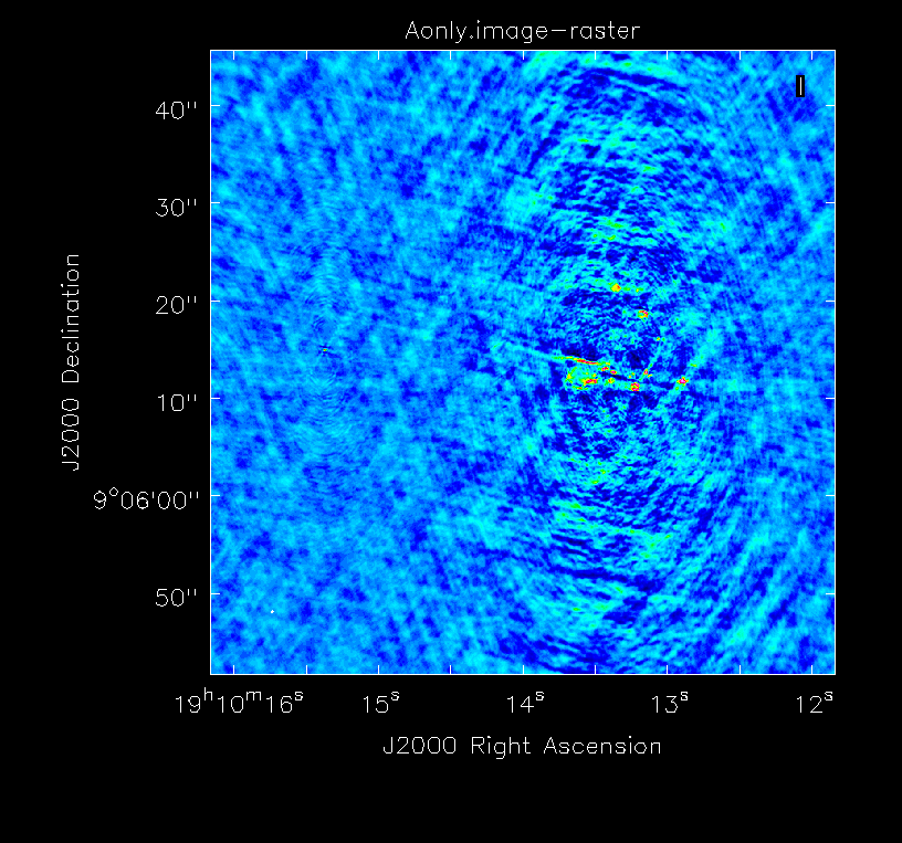
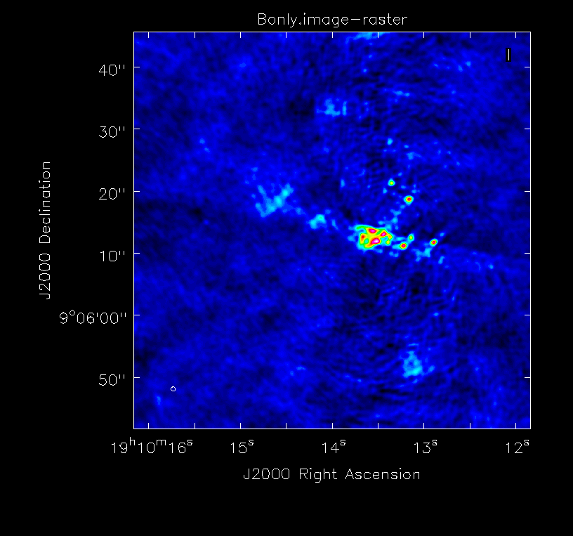
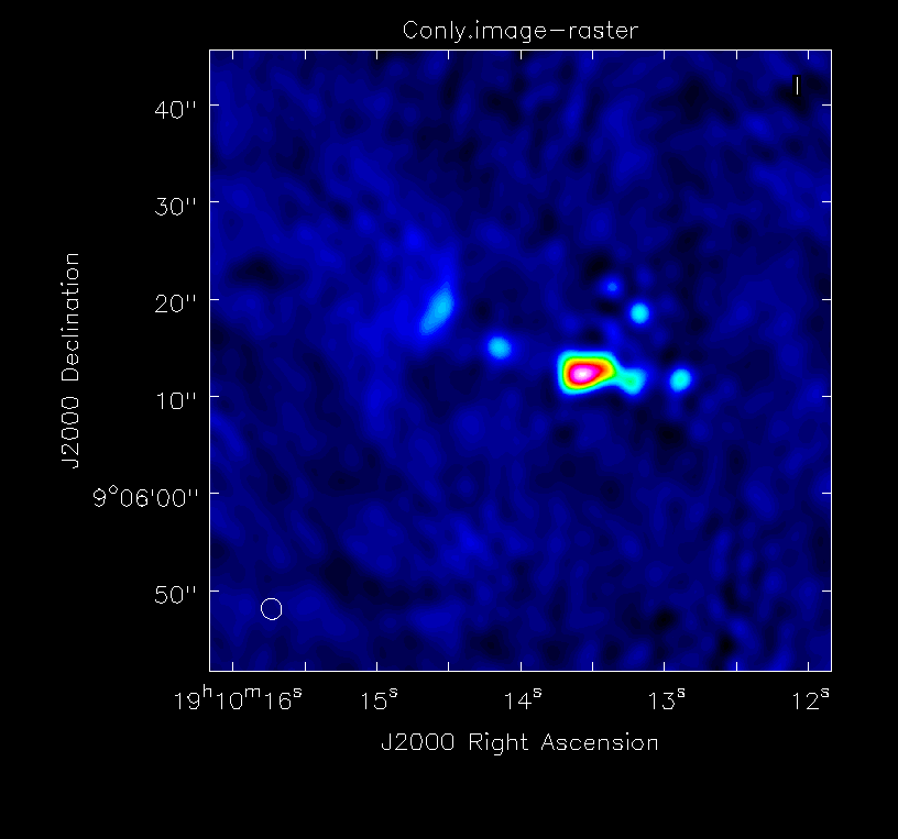
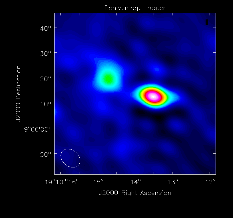
The clean images, shown in Fig. 2a-d, give a first impression of the data. Note that when combining the images, we will improve on the uv-coverage and will therefore not only combine high resolution with high surface brightness sensitivity on large scales, but also expect a higher image fidelity, i.e. fewer artifacts due to better deconvolution. In particular, the ripples in the extended configuration data are the typical 'missing short spacing' bowls, that the more compact configurations will fill in to improve the image quality.
The basic parameters of the individual images can be checked through imhead and the beam sizes are 0.19"x0.19" for A, 0.71"x0.66" for B, 2.20"x2.04" for C and 8.44"x6.36" for D-configuration. This reflects again the factor of three in resolution between the different arrays.
Check and Adjust the Visibility Weights
VLA visibility weights are currently based only on channel width and correlator integration time. In the future, the VLA may use the switched power measurements to derive absolute calibrated weights. At the moment, however, the VLA weights need to be taken as being relative to each other. The relative sensitivity within an observation is measured by the gain, so weights of single, continuous observations are self-consistent. It is important to adjust the weights between separate observations as they will potentially be on different scales.
Let's have a look at the weights of the different datasets. We will plot the weights as a function of uv-distance in a single central channel for improved plotting time:
# In CASA
# A-config:
plotms(vis='A-W49A.ms',spw='0:32',xaxis='uvwave',yaxis='wt',coloraxis='antenna1')
# In CASA
# B-config
plotms(vis='B-W49A.ms',spw='0:32',xaxis='uvwave',yaxis='wt',coloraxis='antenna1')
# In CASA
# C-config:
plotms(vis='C-W49A.ms',spw='0:32',xaxis='uvwave',yaxis='wt',coloraxis='antenna1')
# In CASA
# D-config:
plotms(vis='D-W49A.ms',spw='0:32',xaxis='uvwave',yaxis='wt',coloraxis='antenna1')
Fig. 3a-d shows the weights and they are as described above.
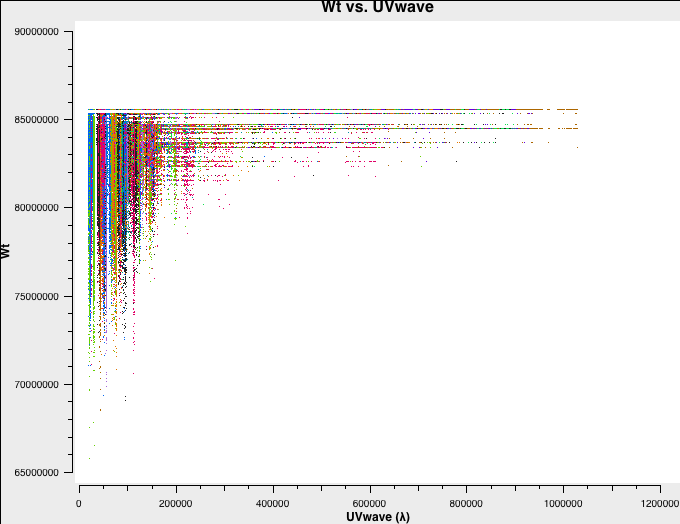 A-config original weights. |
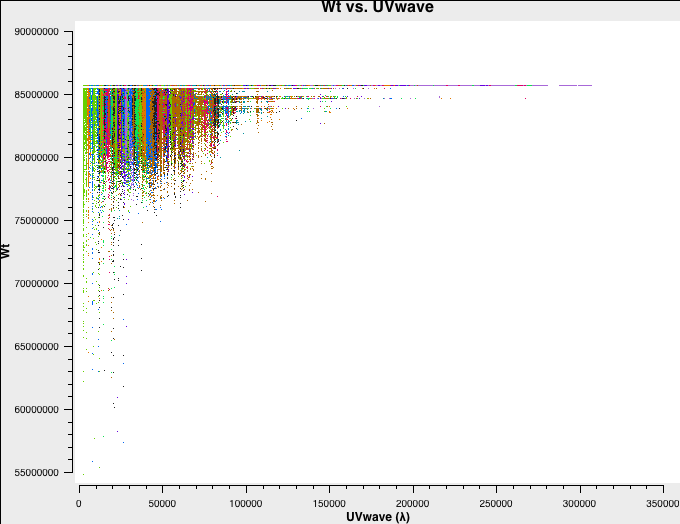 B-config original weights. |
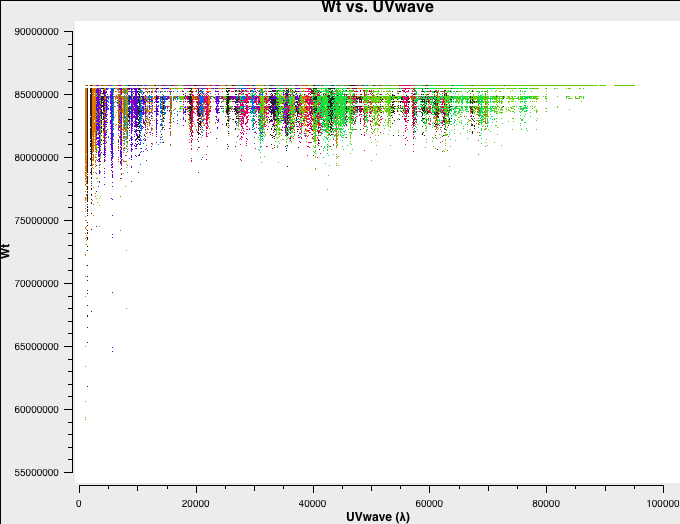 C-config original weights. |
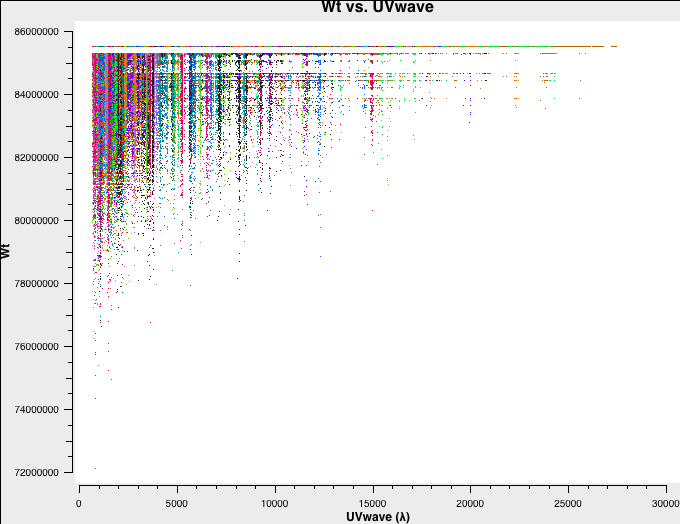 D-config original weights. |
The next step is to bring the weights on the same relative scale.
There are currently a number of options to do so.
1) Calculate the weights based on the rms of the visibilities themselves, using the statwt task.
2) Reset the weights with initweights to reflect the channel width and correlator integration time ([math]\displaystyle{ WEIGHT=2 \Delta \nu \Delta t }[/math], see the document on Data Weights in CASAdocs).
3) Calculate the weights based on the rms of the cross-polarization products (currently not supported in statwt).
We recommend to reset the weights when there are strong sources present in the data as they will change the rms of the visibilities and the rms will not be representative of the noise anymore. Without strong sources, statwt should deliver better results. The third option may work for both cases, but requires full polarization observations and calibrations. For this guide we will follow the statwt path as an example. But the user should be aware of the different options for optimized imaging.
Calculating the weights based on the rms
statwt will bring all the weights of all observations on the same scale. The task recalculates the visibility weights based on the inverse of their rms. Task statwt is part of the VLA pipeline, so the pipelined data may already have recalculated weights and this step can be skipped. It does not hurt though, to re-run statwt. For more information on weights, see definition of data weights.
Task statwt will be executed on each MS. The default setting calculates the weight based on the rms of each scan and spectral window. This setting works quite well for continuum observations. We would like to note though that for spectral line data the fitspw parameter should be set to exclude the line from the calculations. Otherwise, strong lines will be down-weighted.
Now, we execute statwt. Since the DATA column is our calibrated data (see above; in a general case it would be the CORRECTED_DATA column), we calculate the rms based on the values in that column:
# In CASA
# A-config:
statwt(vis='A-W49A.ms',datacolumn='data')

# B-config
statwt(vis='B-W49A.ms',datacolumn='data')

# C-config:
statwt(vis='C-W49A.ms',datacolumn='data')

# D-config:
statwt(vis='D-W49A.ms',datacolumn='data')
Let's have a look at the weight values again to see if statwt has adjusted the weights properly:
# In CASA
# A-config:
plotms(vis='A-W49A.ms',spw='0:32',xaxis='uvwave',yaxis='wt',coloraxis='antenna1')

# B-config
plotms(vis='B-W49A.ms',spw='0:32',xaxis='uvwave',yaxis='wt',coloraxis='antenna1')

# C-config:
plotms(vis='C-W49A.ms',spw='0:32',xaxis='uvwave',yaxis='wt',coloraxis='antenna1')

# D-config:
plotms(vis='D-W49A.ms',spw='0:32',xaxis='uvwave',yaxis='wt',coloraxis='antenna1')
In Fig. 4a-d we plot the new, recalculated weights for the three configurations. The absolute scaling has indeed changed. and is now in units of 1/Jy^2.
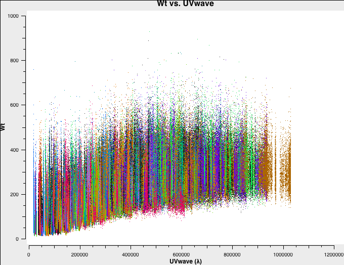 A-config recalculated weights. |
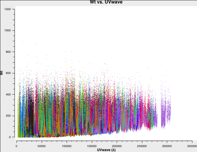 B-config recalculated weights. |
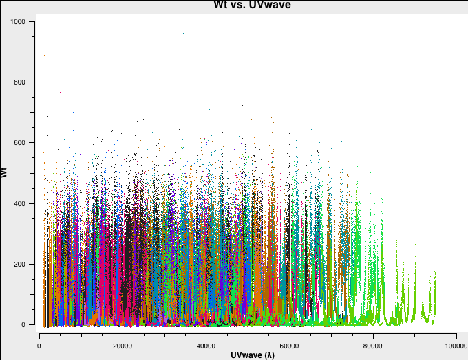 C-config recalculated weights. |
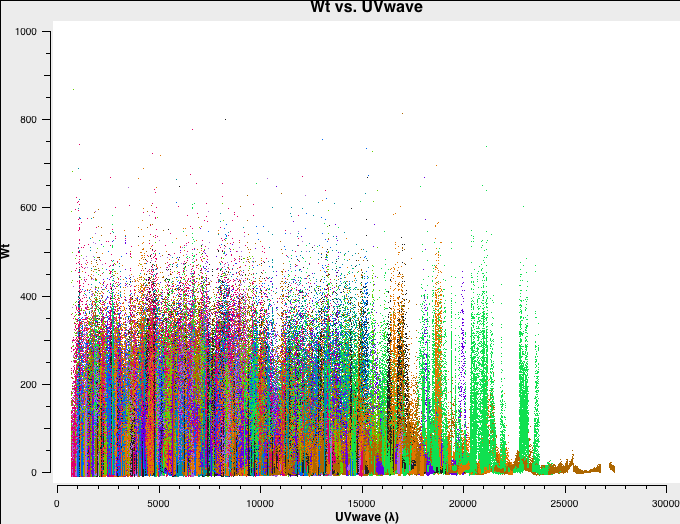 D-config recalculated weights. |
Combining and Imaging All Data
We will now create a combined image of all four re-weighted datasets.
First, let's check the new uv-coverage. We concatenate the data with concat:
# In CASA
concat(vis=['A-W49A.ms','B-W49A.ms','C-W49A.ms','D-W49A.ms'],concatvis='ABCD-W49A.ms')
Now let's plot the uv-coverage of the combined MSs. Since the spws have been renumbered, we plot the central channel of each sub-configuration with the spw='*:32' keyword:
# In CASA
plotms(vis='ABCD-W49A.ms',xaxis='Uwave',yaxis='Vwave',spw='*:32')
Fig. 5 shows the combined uv-coverage, which extends to A-configuration baselines but with a much higher density at the intermediate and short baselines contributed from B, C, and D configurations.
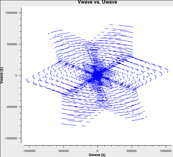 Combined uv-coverage. |
Although concat merges all four MSs into a single one, it is actually not a required step before imaging. Task tclean will take care of the combination when all datasets are specified as a list. Tclean will also perform the spectral regridding of all datasets on the fly, in particular in mode="velocity" or mode="frequency". There's no need to run cvel/cvel2 (or mstransform) to Doppler correct the MSs beforehand.
We will now create a combined image in tclean. The threshold parameter was derived by a previous run of tclean on the combined MS for which we determined the rough rms noise. For our threshold, we will use the rms noise multiplied by a factor of ~2.5.
Image the data with recalculated weights:
# In CASA
tclean(vis=['ABCD-W49A.ms'], imagename='W49A_combinedABCD',specmode='mfs',cell='0.05arcsec',imsize=[1280,1280],
niter=10000, weighting='briggs',robust=0, phasecenter='J2000 19:10:14  +09.06.13.7',threshold='2mJy')
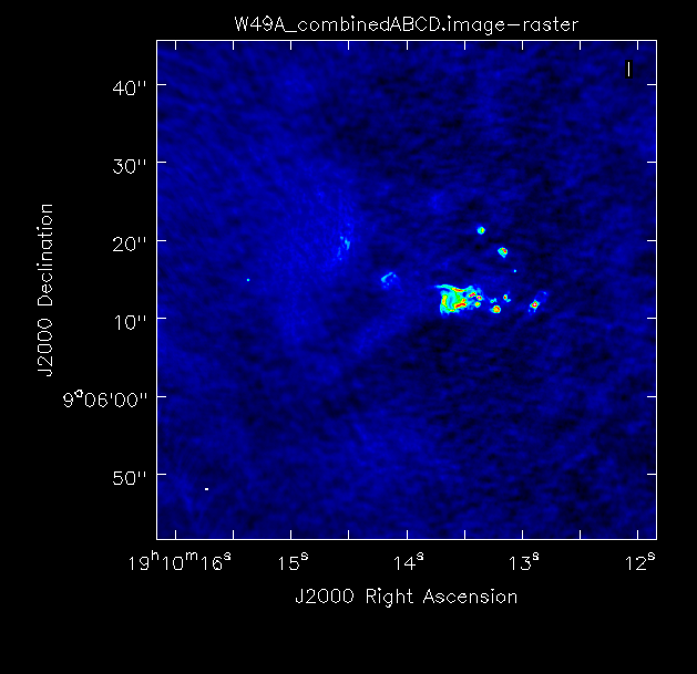 Combined image. |
The combined beam is now 0.26"x0.24". The image (Fig. 6) can still be improved upon. For simplicity, we did not use any interactive cleaning in the above, but we highly recommend it for producing the final images. Improvements can also be obtained by adjusting the image weights via the Briggs robust parameter, adding a taper, or weighting the different datasets against each other using visweightscale in concat. Wide-band imaging and multi-scale imaging will also lead to better results. We refer to the VLA CASA Imaging Guide for more details and examples.
Tips for Selfcal
If the source has a bright nucleus or, more generally, a bright unresolved emission, start with the A array data, selfcal, then add B array, selfcal again, and so on. This procedure starts with a high model flux that is increased further. If the source is mostly diffuse, then there is not much signal in the A array data, so start with the D array, selfcal, then add C array, selfcal, and so on. Each selfcal step should be phase-only first with maybe two or more iterations. At the end of each selfcal step, a phase+amplitude selfcal can be attempted, before merging in the next array configuration data. After each merge the selfcal steps can be repeated. General selfcal procedures are outlined in the Self-Calibration topical guide.
Last checked on CASA Version 6.2.0.
