EVLA Advanced Topics 3C391-CASA4.3: Difference between revisions
No edit summary |
No edit summary |
||
| (8 intermediate revisions by the same user not shown) | |||
| Line 1: | Line 1: | ||
[[Category:EVLA]] | [[Category:EVLA]] | ||
This is the second part of the EVLA 3C391 data reduction tutorial. [http://casaguides.nrao.edu/index.php?title= | This is the second part of the EVLA 3C391 data reduction tutorial. [http://casaguides.nrao.edu/index.php?title=EVLA_Continuum_Tutorial_3C391-CASA4.3 3C391 Tutorial Part 1: calibration, imaging] | ||
<b>This casaguide is for Version 4.3.1 of CASA.</b> If you are using a later version of CASA and this is the most recent | <b>This casaguide is for Version 4.3.1 of CASA.</b> If you are using a later version of CASA and this is the most recent | ||
| Line 8: | Line 8: | ||
= Continuum Observations Data Reduction Tutorial: 3C 391 - Advanced Topics = | = Continuum Observations Data Reduction Tutorial: 3C 391 - Advanced Topics = | ||
In this document, we discuss various "advanced topics" for further reduction of the 3C 391 continuum data. This tutorial assumes that the reader already has some familiarity with basic continuum data reduction, such as should have been obtained in the [[EVLA Continuum Tutorial 3C391 | In this document, we discuss various "advanced topics" for further reduction of the 3C 391 continuum data. This tutorial assumes that the reader already has some familiarity with basic continuum data reduction, such as should have been obtained in the [[EVLA Continuum Tutorial 3C391-CASA4.3 | Continuum Data Reduction Tutorial]]. | ||
<!-- on the first day of the NRAO Synthesis Imaging Workshop data reduction tutorials. --> | <!-- on the first day of the NRAO Synthesis Imaging Workshop data reduction tutorials. --> | ||
== Starting Point == | == Starting Point == | ||
If you finished the [[EVLA Continuum Tutorial 3C391 | If you finished the [[EVLA Continuum Tutorial 3C391-CASA4.3 | Continuum Data Reduction Tutorial]] you will have ended up with a dataset called | ||
<tt>3c391_ctm_mosaic_spw0.ms</tt>. This is what we will use to carry on with our polarization imaging. | <tt>3c391_ctm_mosaic_spw0.ms</tt>. This is what we will use to carry on with our polarization imaging. | ||
| Line 19: | Line 19: | ||
* You can obtain the calibrated split mosaic data from [http://casa.nrao.edu/Data/EVLA/3C391/EVLA_3C391_FinalCalibratedMosaicMS.tgz EVLA_3C391_FinalCalibratedMosaicMS.tgz] (dataset size: 1.3GB). You unpack it using <tt>tar xzf EVLA_3C391_FinalCalibratedMosaicMS.tgz</tt> which will create a subdirectory called <tt>VLA_3C391_FinalCalibratedMosaicMS</tt> with the MS <tt>3c391_ctm_mosaic_spw0.ms</tt> inside it. You can then <tt>cd</tt> into this directory and run <tt>casapy</tt> from there. | * You can obtain the calibrated split mosaic data from [http://casa.nrao.edu/Data/EVLA/3C391/EVLA_3C391_FinalCalibratedMosaicMS.tgz EVLA_3C391_FinalCalibratedMosaicMS.tgz] (dataset size: 1.3GB). You unpack it using <tt>tar xzf EVLA_3C391_FinalCalibratedMosaicMS.tgz</tt> which will create a subdirectory called <tt>VLA_3C391_FinalCalibratedMosaicMS</tt> with the MS <tt>3c391_ctm_mosaic_spw0.ms</tt> inside it. You can then <tt>cd</tt> into this directory and run <tt>casapy</tt> from there. | ||
* One could use the [[Extracting scripts from these tutorials | script extractor]] to generate a CASA reduction script from the [[EVLA Continuum Tutorial 3C391 | * One could use the [[Extracting scripts from these tutorials | script extractor]] to generate a CASA reduction script from the [[EVLA Continuum Tutorial 3C391-CASA4.3 | Continuum Data Reduction Tutorial]] and process the data to form an initial image. Current experience on a standard desktop computer suggests that such a data set could be processed in 30 min. or less. | ||
== Multi-scale Polarization Clean == | == Multi-scale Polarization Clean == | ||
| Line 90: | Line 90: | ||
* <tt>stokes=' '</tt> : This example determines the peak brightness in the <EM>entire</EM> image, which has all four Stokes planes. If one wanted to determine the peak brightness in just, say, the Stokes V image, one would set stokes='V'. | * <tt>stokes=' '</tt> : This example determines the peak brightness in the <EM>entire</EM> image, which has all four Stokes planes. If one wanted to determine the peak brightness in just, say, the Stokes V image, one would set stokes='V'. | ||
The dictionary contains the values which you can extract for further use, for | The dictionary contains the values which you can extract for further use. For example, for a particular instance of | ||
the previous clean, we found: | |||
<pre style="background-color: #E0FFFF;"> | <pre style="background-color: #E0FFFF;"> | ||
CASA <4>: mystat | CASA <4>: mystat | ||
| Line 96: | Line 97: | ||
{'blc': array([0, 0, 0, 0], dtype=int32), | {'blc': array([0, 0, 0, 0], dtype=int32), | ||
'blcf': '18:50:04.251, -01.05.40.567, I, 4.59901e+09Hz', | 'blcf': '18:50:04.251, -01.05.40.567, I, 4.59901e+09Hz', | ||
'flux': array([ | 'flux': array([ 9.50934186]), | ||
'max': array([ 0. | 'max': array([ 0.15526876]), | ||
'maxpos': array([288, 256, 0, 0], dtype=int32), | 'maxpos': array([288, 256, 0, 0], dtype=int32), | ||
'maxposf': '18:49:16.243, -00.55.00.579, I, 4.59901e+09Hz', | 'maxposf': '18:49:16.243, -00.55.00.579, I, 4.59901e+09Hz', | ||
'mean': array([ 0. | 'mean': array([ 0.00089436]), | ||
'medabsdevmed': array([ 0. | 'medabsdevmed': array([ 0.00015567]), | ||
'median': array([ | 'median': array([ 1.27408730e-05]), | ||
'min': array([-0. | 'min': array([-0.00516682]), | ||
'minpos': array([279, | 'minpos': array([279, 429, 0, 0], dtype=int32), | ||
'minposf': '18:49:17.743, -00.47. | 'minposf': '18:49:17.743, -00.47.48.079, I, 4.59901e+09Hz', | ||
'npts': array([ | 'npts': array([ 474784.]), | ||
'quartile': array([ 0. | 'quartile': array([ 0.00031206]), | ||
'rms': array([ 0. | 'rms': array([ 0.00607521]), | ||
'sigma': array([ 0. | 'sigma': array([ 0.00600903]), | ||
'sum': array([ | 'sum': array([ 424.62918042]), | ||
'sumsq': array([ | 'sumsq': array([ 17.52343054]), | ||
'trc': array([479, 479, 3, 0], dtype=int32), | 'trc': array([479, 479, 3, 0], dtype=int32), | ||
'trcf': '18:48:44.407, -00.45.43.065, V, 4.59901e+09Hz'} | 'trcf': '18:48:44.407, -00.45.43.065, V, 4.59901e+09Hz'} | ||
| Line 147: | Line 148: | ||
I -42.9832km/s LSRK RADIO 4.59901e+09 | I -42.9832km/s LSRK RADIO 4.59901e+09 | ||
BrightnessUnit BeamArea Npts Sum FluxDensity | BrightnessUnit BeamArea Npts Sum FluxDensity | ||
Jy/beam | Jy/beam 44.6539 22119 4.242001e+02 9.499733e+00 | ||
Mean Rms Std dev Minimum Maximum | Mean Rms Std dev Minimum Maximum | ||
1.917809e-02 2.799428e-02 2.039361e-02 -2.618031e-03 1.552688e-01 | |||
region count | region count | ||
1 | 1 | ||
</pre> | </pre> | ||
In our example we find a total Flux density of | In our example we find a total Flux density of 9.5 Jy while the max brightness is only 0.155 Jy/beam. Note that the numbers you get may be slightly different depending on how deeply you cleaned. | ||
By contrast, for the rms noise level, one wants load the original (un-pbcor) image and to <em>exclude</em> the source's emission to the extent possible, as the source's emission will bias the estimated noise level high. Likewise, one should avoid the "clean bowl" around the source emission. One can repeat the procedure above, defining a polygonal region, then double clicking inside it, to determine the statistics. You can use the tapedeck to change which Stokes plane you are viewing and double-click in each to get those statistics. For example, from the region selection shown to the right for off-source statistics: | By contrast, for the rms noise level, one wants load the original (un-pbcor) image | ||
<source lang="python"> | |||
# In CASA | |||
viewer('3c391_ctm_spw0_IQUV.image') | |||
</source> | |||
and to <em>exclude</em> the source's emission to the extent possible, as the source's emission will bias the estimated noise level high. Likewise, one should avoid the "clean bowl" around the source emission. One can repeat the procedure above, defining a polygonal region, then double clicking inside it, to determine the statistics. You can use the tapedeck to change which Stokes plane you are viewing and double-click in each to get those statistics. For example, from the region selection shown to the right for off-source statistics: | |||
<pre style="background-color: #E0FFFF;"> | <pre style="background-color: #E0FFFF;"> | ||
---- ---- ---- ---- ---- ---- ---- ---- ---- ---- ---- ---- ---- ---- ---- ---- ---- | ---- ---- ---- ---- ---- ---- ---- ---- ---- ---- ---- ---- ---- ---- ---- ---- ---- | ||
| Line 162: | Line 168: | ||
I -42.9832km/s LSRK RADIO 4.59901e+09 | I -42.9832km/s LSRK RADIO 4.59901e+09 | ||
BrightnessUnit BeamArea Npts Sum FluxDensity | BrightnessUnit BeamArea Npts Sum FluxDensity | ||
Jy/beam | Jy/beam 44.6539 52725 -3.092479e+00 -6.925440e-02 | ||
Mean Rms Std dev Minimum Maximum | Mean Rms Std dev Minimum Maximum | ||
- | -5.865299e-05 5.103085e-04 5.069314e-04 -1.945960e-03 2.282981e-03 | ||
region count | region count | ||
1 | 1 | ||
| Line 173: | Line 179: | ||
Q -42.9832km/s LSRK RADIO 4.59901e+09 | Q -42.9832km/s LSRK RADIO 4.59901e+09 | ||
BrightnessUnit BeamArea Npts Sum FluxDensity | BrightnessUnit BeamArea Npts Sum FluxDensity | ||
Jy/beam | Jy/beam 44.6539 52725 -1.474115e-01 -3.301201e-03 | ||
Mean Rms Std dev Minimum Maximum | Mean Rms Std dev Minimum Maximum | ||
- | -2.795856e-06 5.614272e-05 5.607359e-05 -3.039683e-04 2.997937e-04 | ||
region count | region count | ||
1 | 1 | ||
| Line 184: | Line 190: | ||
U -42.9832km/s LSRK RADIO 4.59901e+09 | U -42.9832km/s LSRK RADIO 4.59901e+09 | ||
BrightnessUnit BeamArea Npts Sum FluxDensity | BrightnessUnit BeamArea Npts Sum FluxDensity | ||
Jy/beam | Jy/beam 44.6539 52725 7.583902e-02 1.698374e-03 | ||
Mean Rms Std dev Minimum Maximum | Mean Rms Std dev Minimum Maximum | ||
1. | 1.438388e-06 5.492329e-05 5.490497e-05 -3.513077e-04 2.247283e-04 | ||
region count | region count | ||
1 | 1 | ||
| Line 195: | Line 201: | ||
V -42.9832km/s LSRK RADIO 4.59901e+09 | V -42.9832km/s LSRK RADIO 4.59901e+09 | ||
BrightnessUnit BeamArea Npts Sum FluxDensity | BrightnessUnit BeamArea Npts Sum FluxDensity | ||
Jy/beam | Jy/beam 44.6539 52725 -3.244009e-01 -7.264784e-03 | ||
Mean Rms Std dev Minimum Maximum | Mean Rms Std dev Minimum Maximum | ||
-6.152697e-06 1.186217e-04 1.184631e-04 -4.345808e-04 3.379770e-04 | |||
region count | region count | ||
1 | 1 | ||
---- ---- ---- ---- ---- ---- ---- ---- ---- ---- ---- ---- ---- ---- ---- ---- ---- | ---- ---- ---- ---- ---- ---- ---- ---- ---- ---- ---- ---- ---- ---- ---- ---- ---- | ||
</pre> | </pre> | ||
Thus the I rms is 0. | Thus the I rms is 0.51 mJy and Q and U rms are around 0.056 mJy. It will be useful later on to have the flat-noise and pb-corrected images available separately along with the statistics. | ||
== Constructing Polarization Intensity and Angle Images == | == Constructing Polarization Intensity and Angle Images == | ||
| Line 208: | Line 214: | ||
At the beginning of this Advanced Tutorial, a full polarization imaging cube of 3C 391 was constructed. This cube has 3 dimensions, the standard two angular dimensions (right ascension, declination) and a third dimension containing the polarization information. Considering the image cube as a matrix, <math>Image[l,m,p]</math>, the <math>l</math> and <math>m</math> axis describe the sky brightness or intensity for the given <math>p</math> axis. If one opens the {{viewer}} and loads the 3C 391 continuum image, the default view contains an "animator" or pane with movie controls. One can step through the polarization axis, displaying the images for the different polarizations. | At the beginning of this Advanced Tutorial, a full polarization imaging cube of 3C 391 was constructed. This cube has 3 dimensions, the standard two angular dimensions (right ascension, declination) and a third dimension containing the polarization information. Considering the image cube as a matrix, <math>Image[l,m,p]</math>, the <math>l</math> and <math>m</math> axis describe the sky brightness or intensity for the given <math>p</math> axis. If one opens the {{viewer}} and loads the 3C 391 continuum image, the default view contains an "animator" or pane with movie controls. One can step through the polarization axis, displaying the images for the different polarizations. | ||
As [[EVLA Continuum Tutorial 3C391 | As [[EVLA Continuum Tutorial 3C391-CASA4.3#Imaging | constructed]], the image contains four polarizations, for the four Stokes parameters, I, Q, U, and V. Recalling the lectures, Q and U describe the linear polarization and V describes the circular polarization. Specifically, Q describes the amount of linear polarization aligned with a given axis, and U describes the amount of linear polarization at a 45 deg angle to that axis. The V parameter describes the amount of circular polarization, with the sign (positive or negative) describing the sense of the circular polarization (right- or left-hand circularly polarized). | ||
In general, few celestial sources are expected to show circular polarization, with the notable exception of masers, while terrestrial and satellite sources are often highly circularly polarized. The V image is therefore often worth forming because any V emission could be indicative of unflagged RFI within the data (or problems with the calibration!). | In general, few celestial sources are expected to show circular polarization, with the notable exception of masers, while terrestrial and satellite sources are often highly circularly polarized. The V image is therefore often worth forming because any V emission could be indicative of unflagged RFI within the data (or problems with the calibration!). | ||
| Line 331: | Line 337: | ||
The two input images could be the two different spectral windows from the 3C391 continuum data set (see below). If the higher-frequency spectral window (spw1) has not yet been reduced, then two images made with different channel ranges from the lower spectral window, spw0, should suffice. In this latter case, the extreme upper and lower channels are suggested, to provide a sufficient lever arm in frequency to measure a believable spectral index. | The two input images could be the two different spectral windows from the 3C391 continuum data set (see below). If the higher-frequency spectral window (spw1) has not yet been reduced, then two images made with different channel ranges from the lower spectral window, spw0, should suffice. In this latter case, the extreme upper and lower channels are suggested, to provide a sufficient lever arm in frequency to measure a believable spectral index. | ||
<b> | <b>Note:</b> It would be desirable to produce the spectral index image through the first-order Taylor term expansion in the MFS imaging. This is unfortunately not available with mosaics in the current version of CASA. Stay tuned. | ||
== Self-Calibration == | == Self-Calibration == | ||
| Line 352: | Line 358: | ||
* Apply these corrections ({{applycal}}) to the DATA column, to form a new CORRECTED_DATA column, <em>overwriting</em> the previous contents of CORRECTED_DATA. | * Apply these corrections ({{applycal}}) to the DATA column, to form a new CORRECTED_DATA column, <em>overwriting</em> the previous contents of CORRECTED_DATA. | ||
The following example begins with the standard data set, 3c391_ctm_mosaic_spw0.ms, resulting from the [[EVLA Continuum Tutorial 3C391 | The following example begins with the standard data set, 3c391_ctm_mosaic_spw0.ms, resulting from the [[EVLA Continuum Tutorial 3C391-CASA4.3 | 3C391 Continuum Tutorial]]. From this we will make an I-only multiscale image (3c391_ctm_spw0_I.image) and in particular the model (3c391_ctm_spw0_I.model) to generate a series of gain corrections (stored in 3C391_ctm_mosaic_spw0.selfcal1), those gain corrections are applied to the data to form a set of self-calibrated data, and new image is then formed (3c391_ctm_spw0_IQUV_selfcal1.image). Note that in the clean before the self-cal, it is important that we only image I so that any cleaned polarization does not affect the gaincal. Note that in CASA 4.0 we first use <tt>delmod</tt> on the MS to get rid of the previous polarized model. | ||
<source lang="python"> | <source lang="python"> | ||
#In CASA | #In CASA | ||
| Line 384: | Line 390: | ||
field='',spw='',selectdata=False, | field='',spw='',selectdata=False, | ||
gaintable= ['3c391_ctm_mosaic_spw0.selfcal1'],gainfield=[''],interp=['nearest'], | gaintable= ['3c391_ctm_mosaic_spw0.selfcal1'],gainfield=[''],interp=['nearest'], | ||
calwt=[False]) | calwt=[False],applymode='calflag') | ||
</source> | </source> | ||
The <tt>CORRECTED_DATA</tt> column of the MS now contains the self-calibrated visibilities, when will now be used by clean. | The <tt>CORRECTED_DATA</tt> column of the MS now contains the self-calibrated visibilities, when will now be used by clean. Note that the | ||
<tt>gaincal</tt> step will report a number of solutions with insufficient SNR. By default with <tt>applymode='calflag'</tt> data with no good solutions will be flagged by <tt>applycal</tt>, in this case you will see it report the flagged fraction increasing from 28% to 43%. This may or may not be a good thing. You can control the action of <tt>applycal</tt> in this regard by changing the value of <tt>applymode</tt>: setting <tt>applymode='calflagstrict'</tt> will be even more stringent about flagging things without valid calibration, while <tt>applymode='calonly'</tt> will calibrate those with solutions while passing through data without unchanged. Note that you can see ahead of time what applycal will do by running with <tt>applymode='trial'</tt> which will do the reporting but nothing else. | |||
{| style="background:#98FB98" | |||
|- | |||
| <b>Questions for the Advanced Student:</b> | |||
* Does allowing applycal to flag the data give better images? | |||
* Or, does using <tt>applymode='calonly'</tt> give improved results? | |||
|- | |||
|} | |||
If you planned on doing multiple iterations of self-cal, you would do another I-only image (e.g. <tt>3c391_ctm_spw0_ms_I_selfcal1</tt>) as that is what is needed for the next step. If you want to just go ahead and see what this selfcal has done, make a full IQUV cube: | If you planned on doing multiple iterations of self-cal, you would do another I-only image (e.g. <tt>3c391_ctm_spw0_ms_I_selfcal1</tt>) as that is what is needed for the next step. If you want to just go ahead and see what this selfcal has done, make a full IQUV cube: | ||
Latest revision as of 20:32, 20 April 2015
This is the second part of the EVLA 3C391 data reduction tutorial. 3C391 Tutorial Part 1: calibration, imaging
This casaguide is for Version 4.3.1 of CASA. If you are using a later version of CASA and this is the most recent available guide, then you should be able to use most, if not all, of this casaguide, as we try to limit script breaking changes in CASA development.
Continuum Observations Data Reduction Tutorial: 3C 391 - Advanced Topics
In this document, we discuss various "advanced topics" for further reduction of the 3C 391 continuum data. This tutorial assumes that the reader already has some familiarity with basic continuum data reduction, such as should have been obtained in the Continuum Data Reduction Tutorial.
Starting Point
If you finished the Continuum Data Reduction Tutorial you will have ended up with a dataset called 3c391_ctm_mosaic_spw0.ms. This is what we will use to carry on with our polarization imaging.
If you have not completed the first part of the EVLA Continuum Data Reduction Tutorial, you have a couple of options (in order of increasing complexity):
- You can obtain the calibrated split mosaic data from EVLA_3C391_FinalCalibratedMosaicMS.tgz (dataset size: 1.3GB). You unpack it using tar xzf EVLA_3C391_FinalCalibratedMosaicMS.tgz which will create a subdirectory called VLA_3C391_FinalCalibratedMosaicMS with the MS 3c391_ctm_mosaic_spw0.ms inside it. You can then cd into this directory and run casapy from there.
- One could use the script extractor to generate a CASA reduction script from the Continuum Data Reduction Tutorial and process the data to form an initial image. Current experience on a standard desktop computer suggests that such a data set could be processed in 30 min. or less.
Multi-scale Polarization Clean
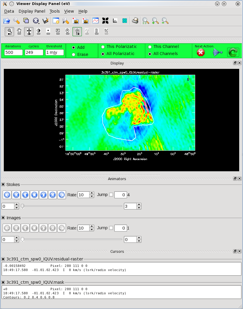
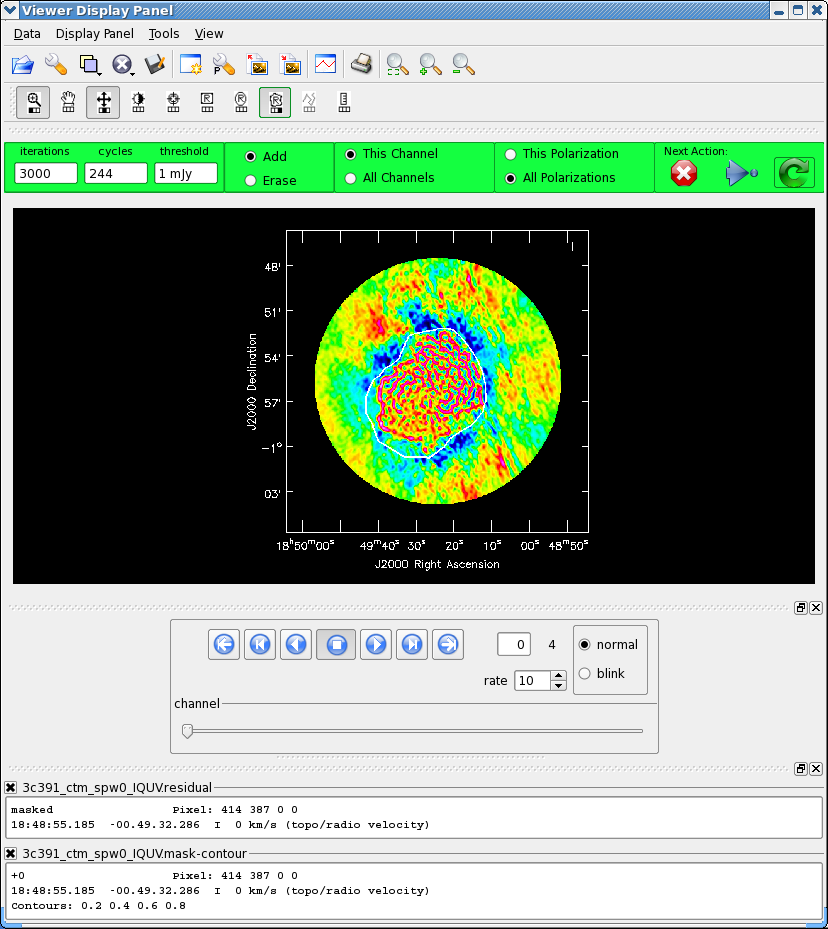
We now employ a multi-scale clean to image Stokes IQUV:
# In CASA
clean(vis='3c391_ctm_mosaic_spw0.ms',imagename='3c391_ctm_spw0_IQUV',
      field='',spw='',
      mode='mfs',
      niter=25000,
      gain=0.1, threshold='1.0mJy',
      psfmode='clarkstokes',
      imagermode='mosaic', ftmachine='mosaic',
      multiscale=[0, 6, 18, 54], smallscalebias=0.9,
      interactive=True,
      imsize=[480,480], cell=['2.5arcsec','2.5arcsec'],
      stokes='IQUV',
      weighting='briggs',robust=0.5,
      pbcor=False,
      usescratch=False)
Warning: This will be significantly slower than in 4.1 due to improvements in the calculation of the frequency-dependent primary beam. For this example it will take around 4-5 minutes to bring up the first image, and something like a few minutes per major cycle.
For these inputs, we have changed:
- stokes='IQUV', psfmode='clarkstokes' : Separate images will be made in all four polarizations (total intensity I, linear polarizations Q and U, and circular polarization V), and, with psfmode='clarkstokes', the Clark CLEAN algorithm will deconvolve each Stokes plane separately thereby making the polarization image more independent of the total intensity.
- multiscale=[0, 6, 18, 54], smallscalebias=0.9 : A multi-scale CLEANing algorithm is used because the supernova remnant contains both diffuse, extended structure on large spatial scales and finer filamentary structure on smaller scales. The settings for multiscale are in units of pixels, with 0 pixels equivalent to the traditional delta-function CLEAN. The scales here are chosen to provide delta functions and then three logarithmically scaled sizes to fit to the data. The first scale (6 pixels) is chosen to be comparable to the size of the beam. The smallscalebias attempts to balance the weight given to larger scales, which often have more flux density, and the smaller scales, which often are brighter. Considerable experimentation is likely to be necessary; one of the authors of this document found that it was useful to CLEAN several rounds with this setting, change to multiscale=[] and remove much of the smaller scale structure, then return to this setting.
- pbcor=False : by default pbcor=False and a flat-noise image is produced. We can do the primary beam correction later (see below).
As previously, we guide the clean using polygon regions in the interactive clean GUI. Because we now have the four Stokes planes in the image for IQUV, you should be sure to extend the mask you draw by selecting the "All Polarizations" radio button before drawing the mask. As you clean, you can use the tapedeck to examine the residuals in the QUV planes. In practice, those will reach the 1 mJy threshold fairly quickly and not be cleaned further while the I cleaning proceeds for a long time. In the screen-shots to the right, you can see that the multiscale clean is doing a better job of picking up the larger-scale emission. After about 15000 iterations the residuals were looking pretty good. As mentioned above restarting clean with different multiscale choices can help also.
After the imaging and deconvolution process has finished, you can use the viewer to look at your image.
# In CASA
viewer('3c391_ctm_spw0_IQUV.image')
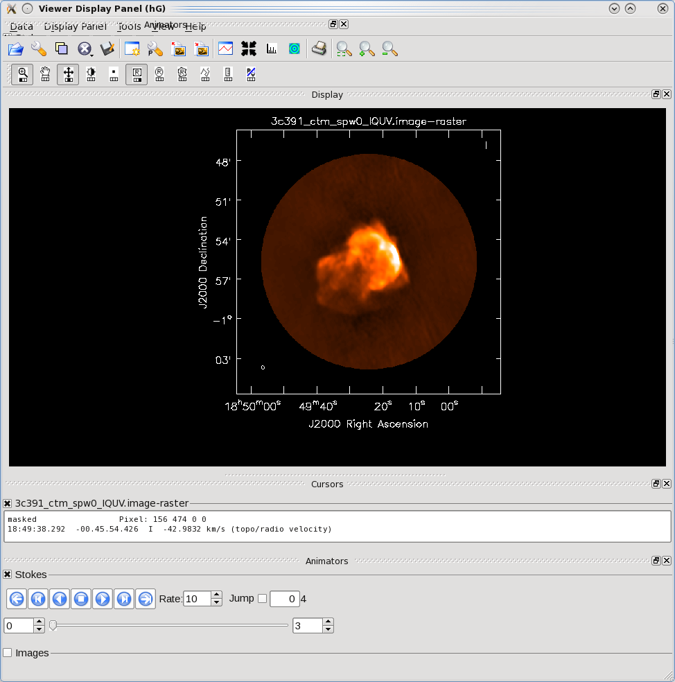
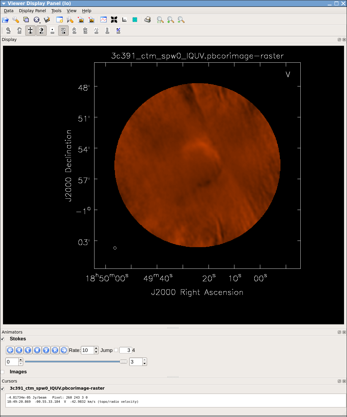
The tape deck buttons that you see under the image can be used to step through the different Stokes parameters (I,Q,U,V). You can adjust the color scale and zoom in to a selected region by assigning mouse buttons to the icons immediately above the image (hover over the icons to get a description of what they do). Also using the "wrench" panel to change Display Options will be helpful here. In the I Stokes plane (1) shown to the right we chose the "Hot Metal 1" colormap. In the lower panel showing the V Stokes plane (3) we also set the "scaling power cycles" to -1.5 to enhance low-contrast emission. Our Stokes I image is significantly better than with just a delta-function classic clean. You can also explore the Q and U images but we will produce more intuitive images from these later on. Finally, note that the residual emission in Stokes V is not real, but likely due to the EVLA "beam squint" between R and L (they are slightly separated on the sky, and this is not currently compensated for in our production version of clean).
The clean task naturally operates in a "flat noise" image, i.e. an image where the effective weighting across the mosaic field of view is set so that the noise is constant. This is so that the clean threshold has a uniform meaning for the stopping criterion and that the image fed into the minor cycles has uniform noise levels. However, this means that the image does not take into account the primary beam fall-off in the edges and interstices of the mosaic. We could have set pbcor=True in clean, but it is useful to see the flat-noise image and residuals to evaluate the quality of the clean image. Therefore, we use immath to divide the .image by the .flux image to produce a primary beam corrected restored image:
# In CASA
immath(outfile='3c391_ctm_spw0_IQUV.pbcorimage',
       mode='evalexpr',
       imagename=['3c391_ctm_spw0_IQUV.image','3c391_ctm_spw0_IQUV.flux'],
       expr="IM0[IM1>0.2]/IM1")
where
- mode='evalexpr' : Use the expr parameter to describe the mathematical operation to perform.
- imagename : A list of images to manipulate, in the order [IM0, IM1, ...] for purposes of expr
- expr : the [Lattice Expression Language] (LEL) expression for the operation. In our case IM0[IM1>0.2]/IM1 means to divide IM0 by IM1 gating on IM1 (and masking outside that).
- outfile : the name of the output image
You can open this in the viewer and see that it has indeed raised the noise (and signal) at the edges of the mosaic.
Image Analysis and Manipulation
This topic is perhaps not "advanced," but it appears to fit more naturally here. It is assumed that an image 3c391_ctm_spw0_IQUV.image, resulting from the above clean, exists.
The three most basic analyses are to determine the peak brightness, the flux density, and the image noise level. These are useful measures of how well one's imaging efforts are in approaching the thermal noise limit or in reproducing what is already known about a source. Additional discussion of image analysis and manipulation, including the combination of multiple images, mathematical operations on images, and much more can be found in Image Analysis in the CASA Reference Book.
The most straightforward statistic is the peak brightness, which is determined by imstat.
mystat = imstat(imagename='3c391_ctm_spw0_IQUV.pbcorimage',stokes='')
- mystat=imstat() : imstat returns a Python dictionary which we capture in the variable mystat
- stokes=' ' : This example determines the peak brightness in the entire image, which has all four Stokes planes. If one wanted to determine the peak brightness in just, say, the Stokes V image, one would set stokes='V'.
The dictionary contains the values which you can extract for further use. For example, for a particular instance of the previous clean, we found:
CASA <4>: mystat
  Out[4]:
{'blc': array([0, 0, 0, 0], dtype=int32),
 'blcf': '18:50:04.251, -01.05.40.567, I, 4.59901e+09Hz',
 'flux': array([ 9.50934186]),
 'max': array([ 0.15526876]),
 'maxpos': array([288, 256,   0,   0], dtype=int32),
 'maxposf': '18:49:16.243, -00.55.00.579, I, 4.59901e+09Hz',
 'mean': array([ 0.00089436]),
 'medabsdevmed': array([ 0.00015567]),
 'median': array([  1.27408730e-05]),
 'min': array([-0.00516682]),
 'minpos': array([279, 429,   0,   0], dtype=int32),
 'minposf': '18:49:17.743, -00.47.48.079, I, 4.59901e+09Hz',
 'npts': array([ 474784.]),
 'quartile': array([ 0.00031206]),
 'rms': array([ 0.00607521]),
 'sigma': array([ 0.00600903]),
 'sum': array([ 424.62918042]),
 'sumsq': array([ 17.52343054]),
 'trc': array([479, 479,   3,   0], dtype=int32),
 'trcf': '18:48:44.407, -00.45.43.065, V, 4.59901e+09Hz'}

CASA <5>: mystat['max'][0]
  Out[5]: 0.15493492782115936
and so the peak flux density is 0.155 Jy/beam (likely in the I Stokes plane).
The other two statistics require slightly more care. The flux density of a source is determined by integrating its brightness or intensity over some solid angle, i.e.,
[math]\displaystyle{ S = \int d\Omega I }[/math]
where [math]\displaystyle{ I }[/math] is the intensity (measured in units of Jy/beam), [math]\displaystyle{ \Omega }[/math] is the solid angle of the source (e.g., number of synthesized beams), and [math]\displaystyle{ S }[/math] is the flux density (measured in units of Jy). In general, if the noise is well-behaved in one's image, when averaged over a reasonable solid angle, the noise contribution should approach 0 Jy. If that is the case, then the flux density of the source is also reported by imstat. However, there are many cases for which a noise contribution of 0 Jy may not be a safe assumption. If one's source is in a complicated region (e.g., a star formation region, the Galactic center, near the edge of a galaxy), a better estimate of the source's flux density will be obtained by limiting carefully the solid angle over which the integration is performed.
Open viewer and use it to display the corrected image
# In CASA
viewer('3c391_ctm_spw0_IQUV.pbcorimage')
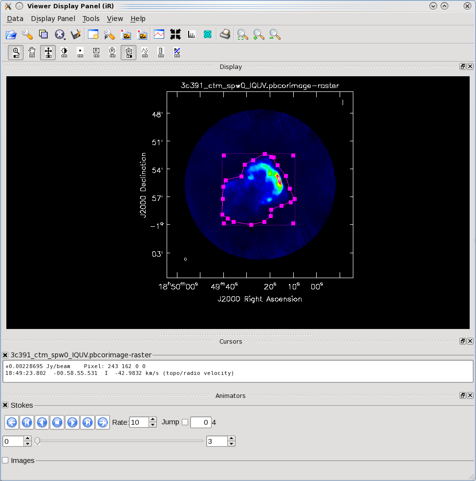
One can choose the function assigned to each mouse button; after zooming into the desired view, assign 'polygon region' to a desired mouse button (e.g., left button) by selecting the icon shown in the figure to the right with the desired mouse button.
Using the mouse button just assigned to 'polygon region', outline the supernova remnant. You start drawing vertices by clicking on points in the image in succession, when you draw the final vertex then you double-click to connect and close the region. When you mouse is inside the region a bounding box will appear with the vertices shown as draggable solid squares. If you want to adjust the vertices you can do so!
If you find you don't like your region you can dismiss it with with ESC key or using the remove region "X" button in lower right of the panel. You can also employ the region panel to save a region you have created, for later use.
Double click inside of that region (using the left mouse button in 4.1), and the statistics will be reported. This will include the flux density value within the region selected.
(3c391_ctm_spw0_IQUV.pbcorimage)
        Stokes       Velocity          Frame        Doppler      Frequency
             I   -42.9832km/s           LSRK          RADIO    4.59901e+09
BrightnessUnit       BeamArea           Npts            Sum    FluxDensity
       Jy/beam        44.6539          22119   4.242001e+02   9.499733e+00
          Mean            Rms        Std dev        Minimum        Maximum
  1.917809e-02   2.799428e-02   2.039361e-02  -2.618031e-03   1.552688e-01
  region count
             1
In our example we find a total Flux density of 9.5 Jy while the max brightness is only 0.155 Jy/beam. Note that the numbers you get may be slightly different depending on how deeply you cleaned.
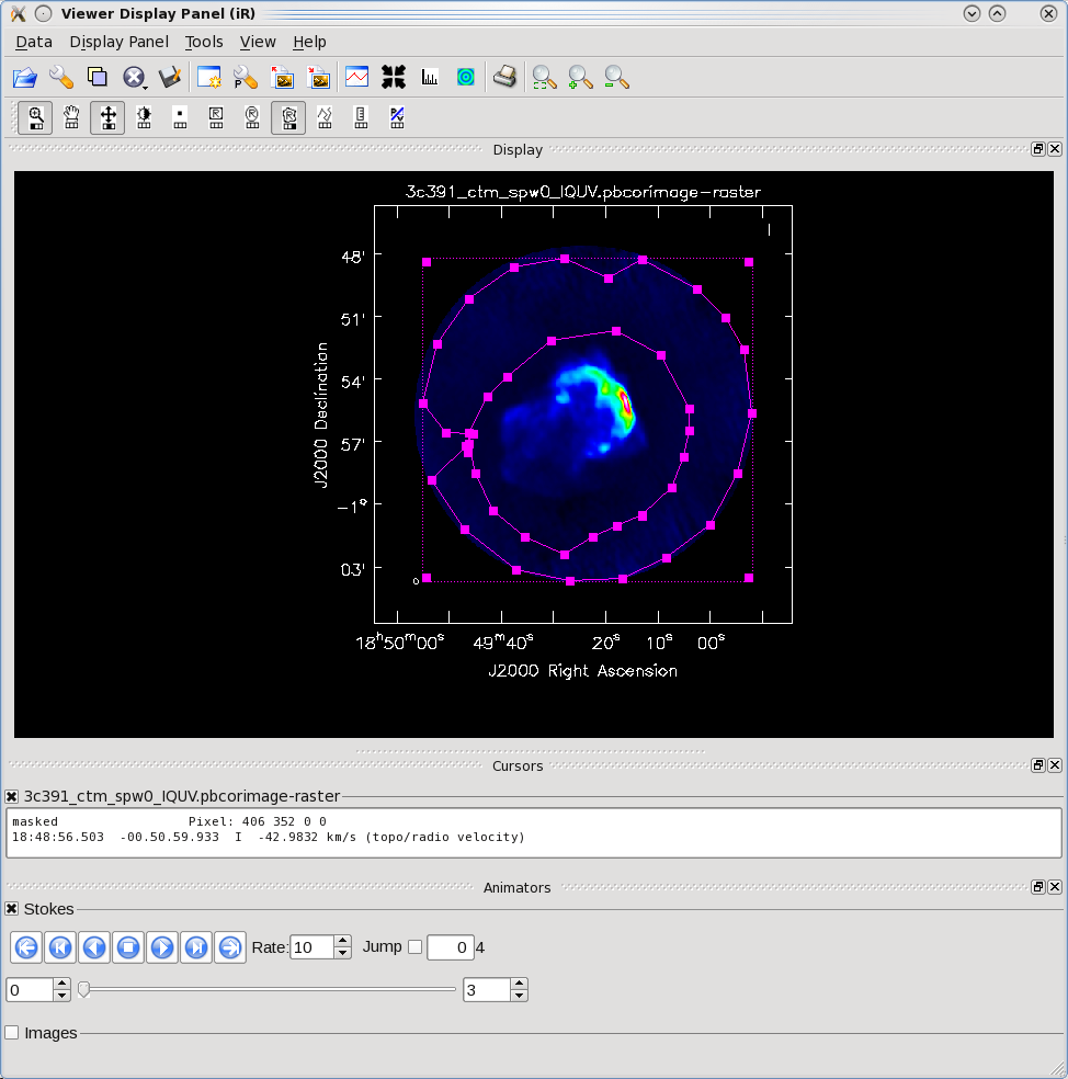
By contrast, for the rms noise level, one wants load the original (un-pbcor) image
# In CASA
viewer('3c391_ctm_spw0_IQUV.image')
and to exclude the source's emission to the extent possible, as the source's emission will bias the estimated noise level high. Likewise, one should avoid the "clean bowl" around the source emission. One can repeat the procedure above, defining a polygonal region, then double clicking inside it, to determine the statistics. You can use the tapedeck to change which Stokes plane you are viewing and double-click in each to get those statistics. For example, from the region selection shown to the right for off-source statistics:
---- ---- ---- ---- ---- ---- ---- ---- ---- ---- ---- ---- ---- ---- ---- ---- ----
(3c391_ctm_spw0_IQUV.image)
        Stokes       Velocity          Frame        Doppler      Frequency
             I   -42.9832km/s           LSRK          RADIO    4.59901e+09
BrightnessUnit       BeamArea           Npts            Sum    FluxDensity
       Jy/beam        44.6539          52725  -3.092479e+00  -6.925440e-02
          Mean            Rms        Std dev        Minimum        Maximum
 -5.865299e-05   5.103085e-04   5.069314e-04  -1.945960e-03   2.282981e-03
  region count
             1
---- ---- ---- ---- ---- ---- ---- ---- ---- ---- ---- ---- ---- ---- ---- ---- ----
---- ---- ---- ---- ---- ---- ---- ---- ---- ---- ---- ---- ---- ---- ---- ---- ----
(3c391_ctm_spw0_IQUV.image)
        Stokes       Velocity          Frame        Doppler      Frequency
             Q   -42.9832km/s           LSRK          RADIO    4.59901e+09
BrightnessUnit       BeamArea           Npts            Sum    FluxDensity
       Jy/beam        44.6539          52725  -1.474115e-01  -3.301201e-03
          Mean            Rms        Std dev        Minimum        Maximum
 -2.795856e-06   5.614272e-05   5.607359e-05  -3.039683e-04   2.997937e-04
  region count
             1
---- ---- ---- ---- ---- ---- ---- ---- ---- ---- ---- ---- ---- ---- ---- ---- ----
---- ---- ---- ---- ---- ---- ---- ---- ---- ---- ---- ---- ---- ---- ---- ---- ----
(3c391_ctm_spw0_IQUV.image)
        Stokes       Velocity          Frame        Doppler      Frequency
             U   -42.9832km/s           LSRK          RADIO    4.59901e+09
BrightnessUnit       BeamArea           Npts            Sum    FluxDensity
       Jy/beam        44.6539          52725   7.583902e-02   1.698374e-03
          Mean            Rms        Std dev        Minimum        Maximum
  1.438388e-06   5.492329e-05   5.490497e-05  -3.513077e-04   2.247283e-04
  region count
             1
---- ---- ---- ---- ---- ---- ---- ---- ---- ---- ---- ---- ---- ---- ---- ---- ----
---- ---- ---- ---- ---- ---- ---- ---- ---- ---- ---- ---- ---- ---- ---- ---- ----
(3c391_ctm_spw0_IQUV.image)
        Stokes       Velocity          Frame        Doppler      Frequency
             V   -42.9832km/s           LSRK          RADIO    4.59901e+09
BrightnessUnit       BeamArea           Npts            Sum    FluxDensity
       Jy/beam        44.6539          52725  -3.244009e-01  -7.264784e-03
          Mean            Rms        Std dev        Minimum        Maximum
 -6.152697e-06   1.186217e-04   1.184631e-04  -4.345808e-04   3.379770e-04
  region count
             1
---- ---- ---- ---- ---- ---- ---- ---- ---- ---- ---- ---- ---- ---- ---- ---- ----
Thus the I rms is 0.51 mJy and Q and U rms are around 0.056 mJy. It will be useful later on to have the flat-noise and pb-corrected images available separately along with the statistics.
Constructing Polarization Intensity and Angle Images
At the beginning of this Advanced Tutorial, a full polarization imaging cube of 3C 391 was constructed. This cube has 3 dimensions, the standard two angular dimensions (right ascension, declination) and a third dimension containing the polarization information. Considering the image cube as a matrix, [math]\displaystyle{ Image[l,m,p] }[/math], the [math]\displaystyle{ l }[/math] and [math]\displaystyle{ m }[/math] axis describe the sky brightness or intensity for the given [math]\displaystyle{ p }[/math] axis. If one opens the viewer and loads the 3C 391 continuum image, the default view contains an "animator" or pane with movie controls. One can step through the polarization axis, displaying the images for the different polarizations.
As constructed, the image contains four polarizations, for the four Stokes parameters, I, Q, U, and V. Recalling the lectures, Q and U describe the linear polarization and V describes the circular polarization. Specifically, Q describes the amount of linear polarization aligned with a given axis, and U describes the amount of linear polarization at a 45 deg angle to that axis. The V parameter describes the amount of circular polarization, with the sign (positive or negative) describing the sense of the circular polarization (right- or left-hand circularly polarized).
In general, few celestial sources are expected to show circular polarization, with the notable exception of masers, while terrestrial and satellite sources are often highly circularly polarized. The V image is therefore often worth forming because any V emission could be indicative of unflagged RFI within the data (or problems with the calibration!).
Because the Q and U images both describe the amount of linear polarization, it is more common to work with a linear polarization intensity image, [math]\displaystyle{ P = \sqrt{Q^2 +U^2} }[/math]. ([math]\displaystyle{ P }[/math] can also be denoted by [math]\displaystyle{ L }[/math].) Also important can be the polarization position angle [math]\displaystyle{ tan 2\chi = U/Q }[/math].
The relevant task is immath, with specific examples for processing of polarization images given in Polarization Manipulation. The steps are the following.
1. Extract the I, Q, U, V planes from the full Stokes image cube, forming separate images for each Stokes parameter. Use the flat-noise images so that non-uniform noise does not bias us.
# In CASA
immath(imagename='3c391_ctm_spw0_IQUV.image',outfile='3c391_ctm_spw0.I',expr='IM0',stokes='I')
immath(imagename='3c391_ctm_spw0_IQUV.image',outfile='3c391_ctm_spw0.Q',expr='IM0',stokes='Q')
immath(imagename='3c391_ctm_spw0_IQUV.image',outfile='3c391_ctm_spw0.U',expr='IM0',stokes='U')
immath(imagename='3c391_ctm_spw0_IQUV.image',outfile='3c391_ctm_spw0.V',expr='IM0',stokes='V')
We also extract a pb-corrected I image for later use:
# In CASA
immath(outfile='3c391_ctm_spw0.pbcorI',
       mode='evalexpr',
       imagename='3c391_ctm_spw0_IQUV.pbcorimage',
       expr='IM0',stokes='I')
2. Combine the Q and U images using the mode='poli' option of immath to form the linear polarization image.
# In CASA
immath(outfile='3c391_ctm_spw0.P',
       mode='poli',
       imagename=['3c391_ctm_spw0.Q','3c391_ctm_spw0.U'],
       sigma='0.0Jy/beam')
Because P is formed from the sum of the squares of the Q and U values, it is biased by the noise. In principle, one can set the sigma value to debias this (it subtracts the square of this value from the Q2+U2 before taking the square-root).
# In CASA
immath(outfile='3c391_ctm_spw0.P_unbias',
       mode='poli',
       imagename=['3c391_ctm_spw0.Q','3c391_ctm_spw0.U'],
       sigma='0.000041Jy/beam')
Currently in CASA 4.1 and earlier, there is a bug where pixels where the noise subtraction makes it negative are set to NaN. To filter this out use immath. Also, you must give sigma in Jy/beam (not mJy/beam). We do:
# In CASA
immath(outfile='3c391_ctm_spw0.P_unbias_filtered',
       mode='evalexpr',
       imagename=['3c391_ctm_spw0.P_unbias'],
       expr="IM0[IM0>-10000.0]")
Finally, one can pb-correct this (after first extracting one plane of the .flux image, they are all the same):
# In CASA
immath(imagename='3c391_ctm_spw0_IQUV.flux',
       outfile='3c391_ctm_spw0.Qflux',
       expr='IM0',stokes='Q')
#
immath(outfile='3c391_ctm_spw0.pbcorP',
       mode='evalexpr',
       imagename=['3c391_ctm_spw0.P_unbias_filtered','3c391_ctm_spw0.Qflux'],
       expr="IM0[IM1>0.2]/IM1")
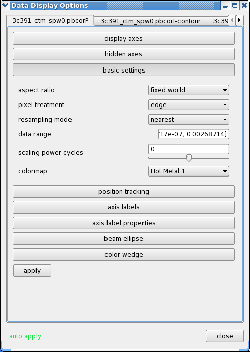
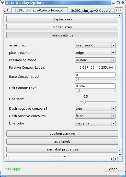
3. Combine the Q and U images using the mode='pola' option of immath to form the polarization position angle image. Because the polarization position angle is derived from the tangent function, the order in which the Q and U images are specified is important. Also, we use the flat-noise images as only the ratio matters and for thresholding you want a uniform noise:
# In CASA
immath(outfile='3c391_ctm_spw0.X',
       mode='pola',
       imagename=['3c391_ctm_spw0.Q','3c391_ctm_spw0.U'],
       polithresh='0.2mJy/beam')
To avoid displaying the position angle of noise, we can set a threshold intensity of the linear polarization for above which we wish to calculate the polarization angle, using the polithresh parameter. An appropriate level here might be the [math]\displaystyle{ 5\sigma }[/math] level of around 0.2 mJy/beam.
4. If desired, form the fractional linear polarization image, defined as P/I. We can do this on the flat-noise image.
# In CASA
immath(outfile='3c391_ctm_spw0.F',
       mode='evalexpr',
       imagename=['3c391_ctm_spw0.I','3c391_ctm_spw0.Q','3c391_ctm_spw0.U'],
       expr='sqrt((IM1^2+IM2^2)/IM0[IM0>1.2e-3]^2)')
Since the total intensity image can (and hopefully does) approach zero in regions free of source emission, dividing by the total intensity can produce very high pixel values in these regions. We therefore wish to restrict our fractional polarization image to regions containing real emission, which we do by setting a threshold in the total intensity image, which in this case corresponds to three times the I noise level. The computation of the polarized intensity is specified by
expr='sqrt((IM1^2+IM2^2)/IM0[IM0>1.2e-3]^2)'
with the expression in square brackets setting the threshold in IM0 (the total intensity image). Note that IM0, IM1 and IM2 correspond to the three files listed in the imagename array, in that order. The order in which the different images are specified is therefore critical once again.
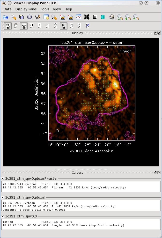
One can then view these various images using viewer. It is instructive to display the I, P and X images (total intensity, total linearly polarized intensity, and polarization position angle) together, to show how the polarized emission relates to the total intensity, and how the magnetic field is structured. We can do this using the viewer.
- Begin by loading the linear polarization image in the viewer:
# In CASA
viewer('3c391_ctm_spw0.pbcorP')
- Next, load the pb-corrected total intensity image as a contour image. In the viewer panel, hit the "Open" icon (the leftmost button in the top row of icons in the viewer). This will bring up a 'Load Data' GUI showing all images and MS in the current directory. Select the total intensity image (3c391_ctm_spw0.pbcorI) and click the 'Contour Map' button on the right hand side.
- Finally, load the polarization position angle image (3c391_ctm_spw0.X) as a vector map.
While we set the polithresh parameter when we created the position angle (X) image, a digression here is instructive in the use of LEL Expressions. Had we not set this parameter, the position angle would have been derived for all pixels within the full IQUV image cube. There is only polarized emission from a limited subset of pixels within this image. Therefore, to avoid plotting vectors corresponding to the position angle of pure noise, we would now wish to select only the regions where the polarized intensity is brighter than some threshold value. To do this, we would use a LEL (Lattice Expression Language) Expression in the 'Load Data' GUI. For our chosen threshold of 0.4 mJy (the 5 sigma level in the pbcorP image), we would paste the expression
'3c391_ctm_spw0.X'['3c391_ctm_spw0.pbcorP'>0.0004]
into the LEL Expression box in the GUI, and click the 'Vector Map' button. This would load the vectors only for regions where [math]\displaystyle{ P\gt 0.4 }[/math] mJy.
While we now have all three images loaded into the viewer (the polarized intensity (3c391_ctm_spw0.pbcorP) in color, the total intensity (3c391_ctm_spw0.pbcorI) as a contour map, and the polarization position angle (3c391_ctm_spw0.X) as a vector map), we still wish to optimize the display for ease of interpretation.
- Click the wrench icon to open a 'Data Display Options' GUI. This will have 3 tabs, corresponding to the three images loaded.
- Change the image transfer function. Hold down the middle mouse button and move the mouse until the color scale is optimized for the display of the polarized intensity. You can change the colormap (e.g. to HotMetal1) in the first tab of the Data Display Options GUI.
- Change the contour levels. Select the total intensity tab (3c391_ctm_spw0.pbcorI) tab (2nd) in the Data Display Options GUI. Change the relative contour levels from the default levels of [0.2,0.4,0.6,0.8,1.0] to powers of [math]\displaystyle{ \sqrt{2} }[/math], including a couple of negative contours at the beginning to demonstrate the image quality. An appropriate set of levels might be [-1.414,-1,1,1.414,2,2.828,4,5.657,8,11.314,16,22.627,32,45.255,64]. These levels will multiply the Unit Contour Level, which we set at some multiple of the rms noise in the total intensity image. An appropriate value might be 0.004 Jy ([math]\displaystyle{ 5\sigma }[/math] of pbcorI rms in the outer part of the mosaic). Choose a nice contour color (e.g. "magenta").
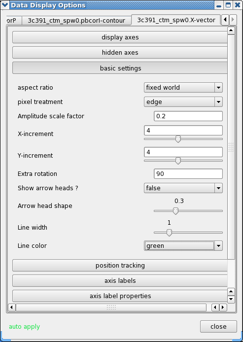
- Change the vector spacing and color, and rotate the vectors. The polarization position angle as calculated is the electric vector position angle (EVPA). If we are interested in the orientation of the magnetic field, then for an optically thin source, the magnetic field orientation is perpendicular to the EVPA, so we must rotate the vectors by [math]\displaystyle{ 90^{\circ} }[/math]. Select the vector image tab in the 'Data Display Options' GUI (labeled as the LEL expression we entered in the Load Data GUI) and enter 90 in the Extra rotation box. If the vectors appear too densely packed on the image, change the spacing of the vectors by setting X-increment and Y-increment to a larger value (4 might be appropriate here). Finally, to be able to distinguish the vectors from the total intensity contours, change the color of the vectors by selecting a different Line color (green might be a good choice).
Now that we have altered the display to our satisfaction, it remains only to zoom in to the region containing the emission. Close the animator tab in the viewer, and then drag out a rectangular region around the supernova remnant with your left mouse button. Double-click to zoom in to that region. This will give you a final image looking something like that shown at right.
Spectral Index Imaging
The spectral index, defined as the slope of the radio spectrum between two different frequencies, [math]\displaystyle{ \log(S_{\nu_1}/S_{\nu_2})/\log(\nu_1/\nu_2) }[/math], is a useful analytical tool which can convey information about the emission mechanism, the optical depth of the source or the underlying energy distribution of synchrotron-radiating electrons.
Having used immath to manipulate the polarization images, the reader should now have some familiarity with performing mathematical operations within CASA. immath also has a special mode for calculating the spectral index, mode='spix' . The two input images at different frequencies should be provided using the parameter (in this case, the Python list) imagename. With this information, it is left as an exercise for the reader to create a spectral index map.
The two input images could be the two different spectral windows from the 3C391 continuum data set (see below). If the higher-frequency spectral window (spw1) has not yet been reduced, then two images made with different channel ranges from the lower spectral window, spw0, should suffice. In this latter case, the extreme upper and lower channels are suggested, to provide a sufficient lever arm in frequency to measure a believable spectral index.
Note: It would be desirable to produce the spectral index image through the first-order Taylor term expansion in the MFS imaging. This is unfortunately not available with mosaics in the current version of CASA. Stay tuned.
Self-Calibration
Recalling the lectures, even after the initial calibration using the amplitude calibrator and the phase calibrator, there are likely to be residual phase and/or amplitude errors in the data. Self-calibration is the process of using an existing model, often constructed by imaging the data itself. Provided that sufficient visibility data have been obtained, and this is essentially always the case with the EVLA (and often the VLBA, and should be with ALMA), the system of equations is wildly over-constrained for the number of unknowns.
More specifically, the observed visibility data on the [math]\displaystyle{ i }[/math]-[math]\displaystyle{ j }[/math] baseline can be modeled as
[math]\displaystyle{ V'_{ij} = G_i G^*_j V_{ij} }[/math]
where [math]\displaystyle{ G_i }[/math] is the complex gain for the [math]\displaystyle{ i^{\mathrm{th}} }[/math] antenna and [math]\displaystyle{ V_{ij} }[/math] is the "true" visibility. For an array of [math]\displaystyle{ N }[/math] antennas, at any given instant, there are [math]\displaystyle{ N(N-1)/2 }[/math] visibility data, but only [math]\displaystyle{ N }[/math] gain factors. For an array with a reasonable number of antennas, [math]\displaystyle{ N }[/math] >~ 8, solutions to this set of coupled equations converge quickly.
There is a small amount of discussion in the CASA Reference Manual on self calibration. In self-calibrating data, it is useful to keep in mind the structure of a Measurement Set: there are three columns of interest for an MS, the DATA column, the MODEL column, and the CORRECTED_DATA column. In normal usage, as part of the initial split, the CORRECTED_DATA column is set equal to the DATA column. The self-calibration procedure is then
- Produce an image (clean) using the CORRECTED_DATA column.
- Derive a series of gain corrections (gaincal) by comparing the DATA columns and the Fourier transform of the image, which is stored in the MODEL column. These corrections are stored in an external table.
- Apply these corrections (applycal) to the DATA column, to form a new CORRECTED_DATA column, overwriting the previous contents of CORRECTED_DATA.
The following example begins with the standard data set, 3c391_ctm_mosaic_spw0.ms, resulting from the 3C391 Continuum Tutorial. From this we will make an I-only multiscale image (3c391_ctm_spw0_I.image) and in particular the model (3c391_ctm_spw0_I.model) to generate a series of gain corrections (stored in 3C391_ctm_mosaic_spw0.selfcal1), those gain corrections are applied to the data to form a set of self-calibrated data, and new image is then formed (3c391_ctm_spw0_IQUV_selfcal1.image). Note that in the clean before the self-cal, it is important that we only image I so that any cleaned polarization does not affect the gaincal. Note that in CASA 4.0 we first use delmod on the MS to get rid of the previous polarized model.
#In CASA
delmod('3c391_ctm_mosaic_spw0.ms')
#
clean(vis='3c391_ctm_mosaic_spw0.ms',imagename='3c391_ctm_spw0_ms_I',
      field='',spw='',
      mode='mfs',
      niter=25000,
      gain=0.1,threshold='1mJy',
      psfmode='clark',
      imagermode='mosaic',ftmachine='mosaic',
      multiscale=[0, 6, 18, 54],smallscalebias=0.9,
      interactive=True,
      imsize=[480,480],cell=['2.5arcsec','2.5arcsec'],
      stokes='I',
      weighting='briggs',robust=0.5,
      usescratch=False)
You don't (or even shouldn't) have to clean extremely deep. You want to be sure to capture as much of the source total flux density as possible, but not include low-level questionable features or sub-structure (ripples) that might be due to calibration or clean artifacts.
After you are happy with the image:
#In CASA
gaincal(vis='3c391_ctm_mosaic_spw0.ms',caltable='3c391_ctm_mosaic_spw0.selfcal1',
        field='',spw='',selectdata=False,
        solint='30s',refant='ea21',minblperant=4,minsnr=3,
        gaintype='G',calmode='p',append=False)
#
applycal(vis='3c391_ctm_mosaic_spw0.ms',
         field='',spw='',selectdata=False,
         gaintable= ['3c391_ctm_mosaic_spw0.selfcal1'],gainfield=[''],interp=['nearest'],
         calwt=[False],applymode='calflag')
The CORRECTED_DATA column of the MS now contains the self-calibrated visibilities, when will now be used by clean. Note that the gaincal step will report a number of solutions with insufficient SNR. By default with applymode='calflag' data with no good solutions will be flagged by applycal, in this case you will see it report the flagged fraction increasing from 28% to 43%. This may or may not be a good thing. You can control the action of applycal in this regard by changing the value of applymode: setting applymode='calflagstrict' will be even more stringent about flagging things without valid calibration, while applymode='calonly' will calibrate those with solutions while passing through data without unchanged. Note that you can see ahead of time what applycal will do by running with applymode='trial' which will do the reporting but nothing else.
Questions for the Advanced Student:
|
If you planned on doing multiple iterations of self-cal, you would do another I-only image (e.g. 3c391_ctm_spw0_ms_I_selfcal1) as that is what is needed for the next step. If you want to just go ahead and see what this selfcal has done, make a full IQUV cube:
#In CASA
clean(vis='3c391_ctm_mosaic_spw0.ms',imagename='3c391_ctm_spw0_IQUV_selfcal1',
      field='',spw='',
      mode='mfs',
      niter=25000,
      gain=0.1,threshold='1mJy',
      psfmode='clarkstokes',
      imagermode='mosaic',ftmachine='mosaic',
      multiscale=[0, 6, 18, 54],smallscalebias=0.9,
      interactive=True,
      imsize=[480,480],cell=['2.5arcsec','2.5arcsec'],
      stokes='IQUV',
      weighting='briggs',robust=0.5,
      usescratch=False)
Questions for the Advanced Student:
|
Commonly, this procedure is applied multiple times. The number of iterations is determined by a combination of the data quality and number of antennas in the array, the structure of the source, the extent to which the original self-calibration assumptions are valid, and the user's patience. With reference to the original self-calibration equation above, if the observed visibility data cannot be modeled well by this equation, no amount of self-calibration will help. A not-uncommon limitation for moderately high dynamic range imaging is that there may be baseline-based factors that modify the "true" visibility. If the corruptions to the "true" visibility cannot be modeled as antenna-based, as they are above, self-calibration won't help.
Self-calibration requires experimentation. Do not be afraid to dump an image, or even a set of gain corrections, change something and try again. Having said that, here are several general comments or guidelines:
- Bookkeeping is important! Suppose one conducts 9 iterations of self-calibration. Will it be possible to remember one month later (or maybe even one week later!) which set of gain corrections and images are which? In the example above, the descriptor 'selfcal1' is attached to various files to help keep straight which is what. Successive iterations of self-cal could then be 'selfcal2', 'selfcal3', etc.
- Care is required in the setting of imagename. If one has an image that already exists, CASA will continue CLEANing it (if it can), which is almost certainly not what one wants during self-calibration. Rather one wants a unique imagename for each pass of self-calibration.
- A common metric for whether self-calibration is whether the image dynamic range (= max/rms) has improved. An improvement of 10% is quite acceptable.
- Be careful when making images and setting CLEAN regions or masks. Self-calibration assumes that the model is "perfect." If one CLEANs a noise bump, self-calibration will quite happily try to adjust the gains so that the CORRECTED_DATA describe a source at the location of the noise bump. As the author demonstrated to himself during the writing of his thesis, it is quite possible to take completely noisy data and manufacture a source. It is far better to exclude some feature of a source or a weak source from initial CLEANing and conduct another round of self-calibration than to create an artificial source. If a real source is excluded from initial CLEANing, it will continue to be present in subsequent iterations of self-calibration; if it's not a real source, one probably isn't interested in it anyway.
- Start self-calibration with phase-only solutions (calmode='p' in gaincal). As Rick Perley has discussed in previous summer school lectures, a phase error of 20 deg is as bad as an amplitude error of 10%.
- In initial rounds of self-calibration, consider solution intervals longer than the nominal sampling time (solint in gaincal) and/or lower signal-to-noise ratio thresholds (minsnr in gaincal). Depending upon the frequency and configuration and fidelity of the model image, it can be quite reasonable to start with solint='30s' or solint='60s' and/or minsnr=3 (or even lower). One might also want to consider specifying a uvrange, if, for example, the field has structure on large scales (small [math]\displaystyle{ u }[/math]-[math]\displaystyle{ v }[/math]) that is not well represented by the current image.
- The task applycal will flag data with no good calibration solutions. During the initial self-calibration steps, this flagging may be excessive. If so, one can restore the flags to the state right before running applycal by using the task flagmanager.
- One can track the agreement between the DATA, CORRECTED_DATA, and MODEL in plotms. The options in 'Axes' allows one to select which column is to be plotted. If the MODEL agrees well with the CORRECTED_DATA, one can use shorter solint and/or higher minsnr values.
- One should consider examining the solutions from gaincal, using plotcal, in order to assure one's self that the corrections are sensible. Smoothly varying phases are good, jumps are usually not. (However, because the phases are often plotted +/- 180 degrees, there can be apparent "jumps," if the phases are very near +180 deg or -180 deg.)
- In the case of a mosaic, such as here, one should also verify that the solutions are of equal quality for all of the fields.
On Your Own: 3C391 second frequency and G93.3+6.9
Now that you have run through spw 0 of 3C391, you are ready to strike off on your own with other datasets. We have provided two options here, described below. The first option is simplest as it is the same object (different spectral window). But for a more rewarding challenge try the L-band dataset on G93.3+6.9!
You can find the data in the CASA repository. Both datasets are contained in this "tarball". Note that these MSes do not have the scratch columns pre-made (to keep the sizes small) so you can do an inintial clearcal to force the creation (or wait until you first calibration task does it for you).
1. 3C391 spw 1 (at 7.5 GHz)
This is the second spectral window split off from the 3C391 dataset. You can process this as you did the first, but beware of RFI in this band! You will have to avoid it (through channel ranges) and/or edit it out. Once you have processed this data and imaged it, you can combine those images in immath to make a spectral index image (see above), or combine the two calibrated MSes in clean to make a deeper MFS image (this might be tricky). You can also look for signs of Faraday Rotation by searching for a polarization angle change between the two spw. Can you derive the "rotation measure" (RM)?
2. Supernova Remnant G93.3+6.9 at L-band
This is data taken at L-band of an entirely different Supernova Remnant, centered near 1400 MHz. You should be able to process this data in a very similar manner to the C-band data on 3C391. Note that we are not telling you what you will see in the image ahead of time - you'll have to try it to see! Here are some data reduction hints to help you along:
- There is strong RFI in this spectral window of the original 2 spw dataset. You will need to find it (e.g. using plotms) and avoid it in imaging. You can also flag those channels using flagdata, but this is not necessary. Note that there is a single baseline that shows very strong interference, see if you can find it! You can flag it using the baseline syntax in flagdata (e.g. antenna='ea0x&ea0y').
- We have not edited out bad or dead antennas for you (unlike in 3C391). You will need to find these using plotms and then flagdata them. One helpful plotms trick is to set antenna='ea01' and pick a few channels (like spw='0:30~33') and a single scan (e.g. scan='2~3') and plot the amp versus Antenna2 on the x-axis. You should see the bad antennas (the low ones). As a check set antenna='ea02' and repeat. Is it the same?
- In spite of RFI, the antenna-based calibration is remarkably resilient to moderate to low RFI contamination (which tends to be baseline-based). So rather than flagging channels with RFI, you might try going ahead with calibration and seeing if the solutions make sense. We were able to calibrate this data without flagging channels (only getting the bad baseline noted above).
- There is no observation of a flux or polarization angle calibrator like J1331+3030. You need to use setjy to set the I flux of the gain calibrator. We use the approximate flux density of 5.8 Jy for J2038+5119.
- When it comes time to calibrate the polarization leakage, we are in good shape since J2038+5119 was observed through a range of parallactic angle (use plotms to plot versus ParAngle). Use poltype='Df+QU' to solve for leakage and the unknown polarization of this source. We do not know the true polarization angle of this source, so before doing poltype='Xf' use setjy to set the Q flux to 5.8Jy * fractional pol (determined in leakage polcal run). This will at least align the polarization when you image it.
- The L-band field of view is much larger than at C-band. From the VLA Observational Status Summary (OSS) the resolution should be around 45" in D-config. Use a cellsize of 15" or smaller. What is the primary beam of the VLA at 1.4MHz? How big should you make your image?
- As you clean you will see faint sources all over the field. Welcome to L-band imaging! This SNR has lots of structure - try both standard and multi-scale clean.
3C391 Line studies
A second data set on 3C391 was taken, this time in OSRO-2 mode, centered on the formaldehyde line at 4829.66 MHz, to search for absorption against the supernova remnant. Again, we made a 7-pointing mosaic, with the same pointing centers as the continuum data set. If you have also already gone through the EVLA high frequency Spectral Line tutorial - IRC+10216 tutorial, then having reduced the continuum data in the EVLA Continuum Tutorial 3C391, you should be able to combine what you have learned from these two tutorials to reduce this spectral line study of 3C 391. Should you wish to do so, a 10-s averaged data set, with some pre-flagging done, is available from the CASA repository.
Last checked on CASA Version 4.3.1.